An Automatic Search and Energy-Saving Continuous Tracking Algorithm for Underwater Targets Based on Prediction and Neural Network

Abstract

Underwater target search and tracking has become a technical hotspot in underwater sensor networks (UWSNs). Unfortunately, the complex and changeable marine environment creates many obstacles for localization and tracking. This paper proposes an automatic search and energy-saving continuous tracking algorithm for underwater targets based on prediction and neural network (ST-BPN). Firstly, the network contains active sensor nodes that can transmit detection signal. When analyzing the reflected signal spectrum, a modified convolutional neural network M-CNN is built to search the target. Then, based on the relationship between propagation delay and target location, a localization algorithm which can resist the influence of clock asynchrony LA-AIC is designed. Thirdly, a scheme based on consensus filtering TS-PSMCF is used to track the target. It is worth mentioning that a predictive switching mechanism, PSM, is added to the tracking process to adjust the working state of nodes. Simulation results show that the recognition accuracy of M-CNN is as high as 99.7%, the location accuracy of LA-AIC is 92.3% higher than that of traditional methods, and the tracking error of TS-PSMCF is kept between 0 m and 5 m.

1. Introduction

The continuous consumption of earth resources must accompany the development of society. The exploitation of land resources has reached a stalemate, and humanity has gradually shifted its focus to the vast ocean [1]. In order to realize the monitoring of underwater area, UWSNs technology came into being [2,3,4,5]. When using UWSNs to realize the application of anti-submarine intrusion detection, underwater field control, and unknown target detection in the military field, as well as marine environmental pollution detection, resource detection, and scientific research experiment in the civil field, there are many technical obstacles in the vast dynamic system of the ocean [6,7]. Underwater target detection, localization, and tracking is one of the key technologies of UWSNs. The research on this technology is helpful to realize various underwater applications.

It is possible to classify underwater target detection and localization technology based on whether the targets can send localization requests. The first and most well-known scheme is the passive detection and localization scheme. As we all know, the first proposed arrival direction scheme (DoA) [8], signal transmission and reception strength scheme (RSSI) [9], arrival time scheme (ToA) [10], and Doppler frequency shift scheme [11] belong to this category. These localization schemes have high location accuracy, but they require high computing power and energy of equipment, and the deployment cost brings economic pressure. Fortunately, a scheme called active detection and localization is proposed. Its basic principle is that nodes send localization signals actively. After these detection signals hit the target, they will be reflected, and other nodes can receive the reflected signals. Through the analysis and processing of the reflected signal, the coordinates and velocity information of the target can be estimated.

Acoustic signals become the primary mode of transmission in the complex marine environment. The acoustic signal used by sensor nodes must have a wide dynamic range and a low duty cycle. Then, advanced continuous active sonar (CAS) becomes the first choice. This is because CAS has many advantages over traditional pulse active sonar (PAS) [12]. The experimental part of the previous paper [13] proves that CAS can achieve better experimental results than PAS. The linear frequency modulation (LFM) signal in CAS can balance the resolution in two classical domains. LFM is used as target detection [14], and a Doppler filter with hysteresis is used for estimation. Its disadvantage is non-adaptive. Facing the challenge of high complexity of signal processing, fractional Fourier transform (FrFT) scheme has brought inspiration. Two discrete fast FrFT algorithms involved in the previous paper [15] can be applied to this. Although the fast discretization algorithm solves the problem of computational complexity to a great extent, the dimension range of two-dimensional spectrum is still beyond imagination. In the development of acoustic wave processing, the dynamics of three-dimensional nonlinear ion acoustic wave in unmagnetized plasma is analyzed in the previous paper [16], while the characteristics of related equations controlling the propagation and diffraction of acoustic beam are studied in the previous paper [17]. If there are multiple targets that need to be located, the difficulty of the problem will continue to escalate.

In view of the problems encountered in the above signal analysis, target detection technology can solve them all [18,19]. In recent years, target detection based on neural network has become a hot research direction in the field of computer vision. Its design idea is to recognize and locate the target in the input image. Convolutional neural network (CNN) is widely used in image fields, especially in image recognition. The combination of VGG16 and CNN in the previous paper [20] can be used for face recognition, and the discarded image information can also be applied to the training process of the original CNN. CNN can also be used for fault detection. Experiments in the previous paper [21] show that it can resist the mutation of workload. A novel region based CNN crack detector with deformable module is proposed in the previous paper [22]. In the application of physics, neural network can be used to establish a model [23]. Combined with particle optimizer, the model can approach the global optimal solution. The analysis of chemical images is also inseparable from the application of CNN. In the previous paper [24], CNN was used to determine the accurate variable measure and fault-tolerant edge dimension of stupid tripod structure. Meyer wavelet can be regarded as CNN [25]. This new CNN can find the numerical solution of fractional pantograph singular system.

For underwater communication, an acoustic signal is the preferred carrier. Its actual delay is 1500 m/s. This communication delay is five times that of radio communication in the air, although the RSSI in the classical algorithm does not have strict requirements for clock synchronization [26]. However, there are too many interference factors in the water, so its location accuracy is low. For the problem of clock asynchrony, how to design an accurate localization algorithm against clock asynchrony interference has become an urgent problem to be solved.

After the target has been precisely located, tracking algorithms based on UWSNs emerge indefinitely. An algorithm based on adaptive Kalman filter is used to track moving targets [27]. It skillfully uses a sleep/wake mechanism to balance tracking accuracy and energy consumption. A tracking algorithm based on extended Kalman filter is proposed [28], and its main purpose is to control energy consumption. Facing the influence of uncertain noise, a scheme using particle filter to complete the tracking task is proposed [29], which is characterized by the depth adjustment mechanism of sensor nodes. In the previous paper [30], Bayesian posterior probability density information was combined with target tracking scheme in order to improve the accuracy of the tracking scheme and its anti-interference ability. A hybrid network architecture, including three types of nodes, is designed [31], in which one type of node acts as data collection, and particle filter algorithm is used. This is a centralized tracking strategy which greatly shortens the node life and is not conducive to the network environment of long-term operation. The corresponding distributed algorithm [32] shares information in the network. However, fusion and sharing will lead to large energy consumption.

It should be noted that there are numerous underwater interference factors, such as bubbles produced by aquatic organism movement, periodic movement of tides, deep-sea currents, and man-made noise. These uncontrollable interference factors will affect the tracking accuracy of the target seriously. Fortunately, the consensus algorithm can adapt to the complex environmental conditions of interference factors effectively [33]. However, this kind of algorithm has high energy consumption. If we can comprehensively consider the needs of tracking accuracy and energy consumption, it is of great significance to design an energy-saving high-precision algorithm for continuous tracking.

This paper designs an automatic search and energy-saving continuous tracking algorithm for underwater targets based on prediction and neural network. We divided the whole algorithm into two important steps: target localization and tracking. In the stage of target localization search, M-CNN is used to detect the rough location of the target. And LA-AIC is used to locate the target accurately. For the tracking stage after target determination, we design TS-PSMCF. In the process of tracking, the method of predicting trajectory is used to adjust the working state of the sensor. This scheme is called PSM. In short, the main contributions of this paper are summarized as follows:

(1)

M-CNN is built to identify the peak position of the spectrum, which can complete the preliminary rough position estimation of the target. The use of M-CNN reduces the computational complexity caused by large-area fine sampling. Even if the spectrum is under sampled, M-CNN can still accurately identify the "hourglass" pattern in the spectrum, which undoubtedly increases the accuracy of target detection.

(2)

LA-AIC is designed to accurately locate the detected target. The relationship equation between time delay and position of target is established. LA-AIC uses the relationship equation to complete localization. LA-AIC not only eliminates the delay problem, but also improves the location accuracy.

(3)

The concept of consensus is introduced into the information fusion algorithm of multi-sensor nodes, and TS-PSMCF is designed. The consensus scheme in TS-PSMCF improves the accuracy in the tracking process. PSM dynamically adjusts the state of each sensor node according to the prediction of target trajectory. In this way, the node without target tracking task can be in the standby state with low energy consumption. Finally, it can save node energy consumption and prolong the life of the whole network.

The rest of this paper is summarized as follows: the model involved in this paper and an overview of ST-BPN are described in the second part. The third part describes the algorithm of underwater target detection and localization. The algorithm of continuous tracking of underwater targets is explained in the fourth part. The experimental verification and analysis are in the fifth part. Finally, the summary of the full text is written in the sixth part.

2. Model and ST-BPN

(1)

Network Model

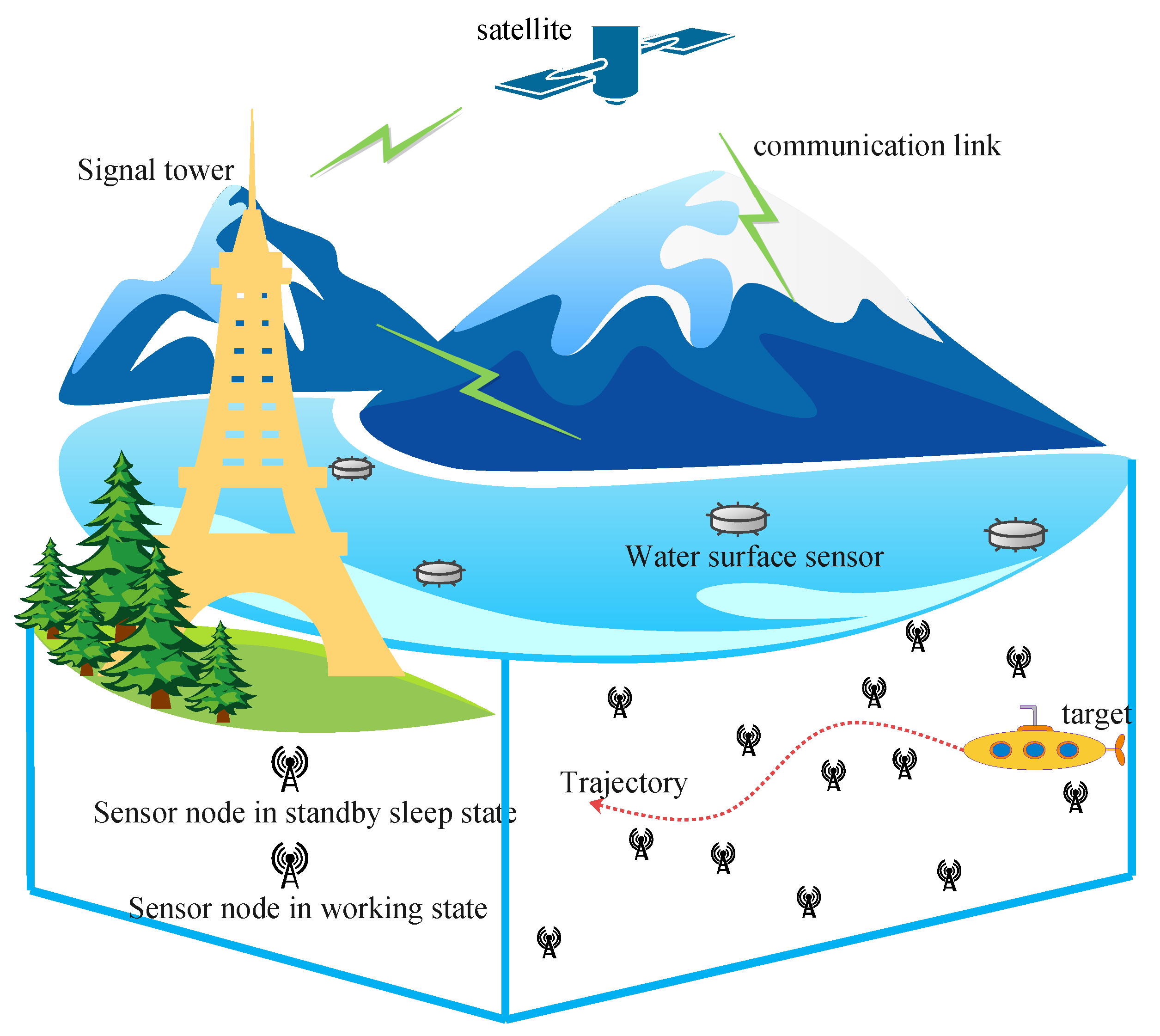
The network structure of UWSNs is shown in Figure 1. The signal tower, satellite, and water surface sensors form a triangular communication link structure. Radio communication is used between them. The signal tower processes the data and has strong computing power. The satellite provides GPS localization information for the sensors on the water surface, and it also can communicate with the signal tower. The surface sensor can complete the localization task and provide clock synchronization service for the underwater sensor nodes [34]. In the monitoring area below the water surface, dynamic targets will be detected, located, and tracked. Some active sensor nodes periodically transmit detection signals to detect targets. Many underwater sensor nodes can communicate with each other, forming many crisscross communication links. The whole underwater network can be represented by communication directed graph $\Phi =\left\{\Gamma ,\Omega \right\}$. The underwater sensor nodes are $\Gamma =\{1,2,3,4,$$...,M\}$, and M is the total number of underwater nodes. The set of communication links is expressed in the form of $\Omega \subset \Gamma \times \Gamma$, which represents that the sensor nodes at both ends of the link can communicate. For each underwater sensor node, if they can carry out one hop communication with another node, they belong to a relationship called “neighbor”. That is, for sensor node $a\left(a\in \Gamma \right)$, its neighbors constitute a set ${\xi }_a=\left\{c\in \Gamma :\left(c,a\right)\in \Omega ,c\ne a\right\}$.

(2)

Detection Model

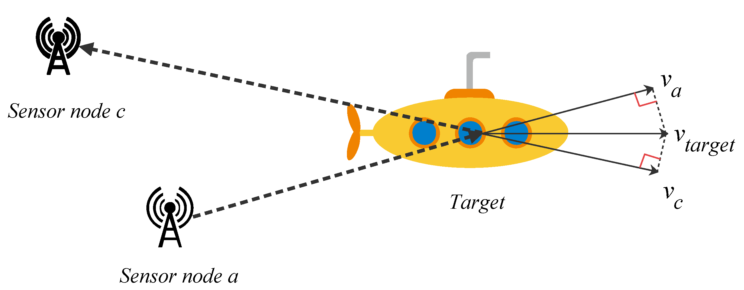
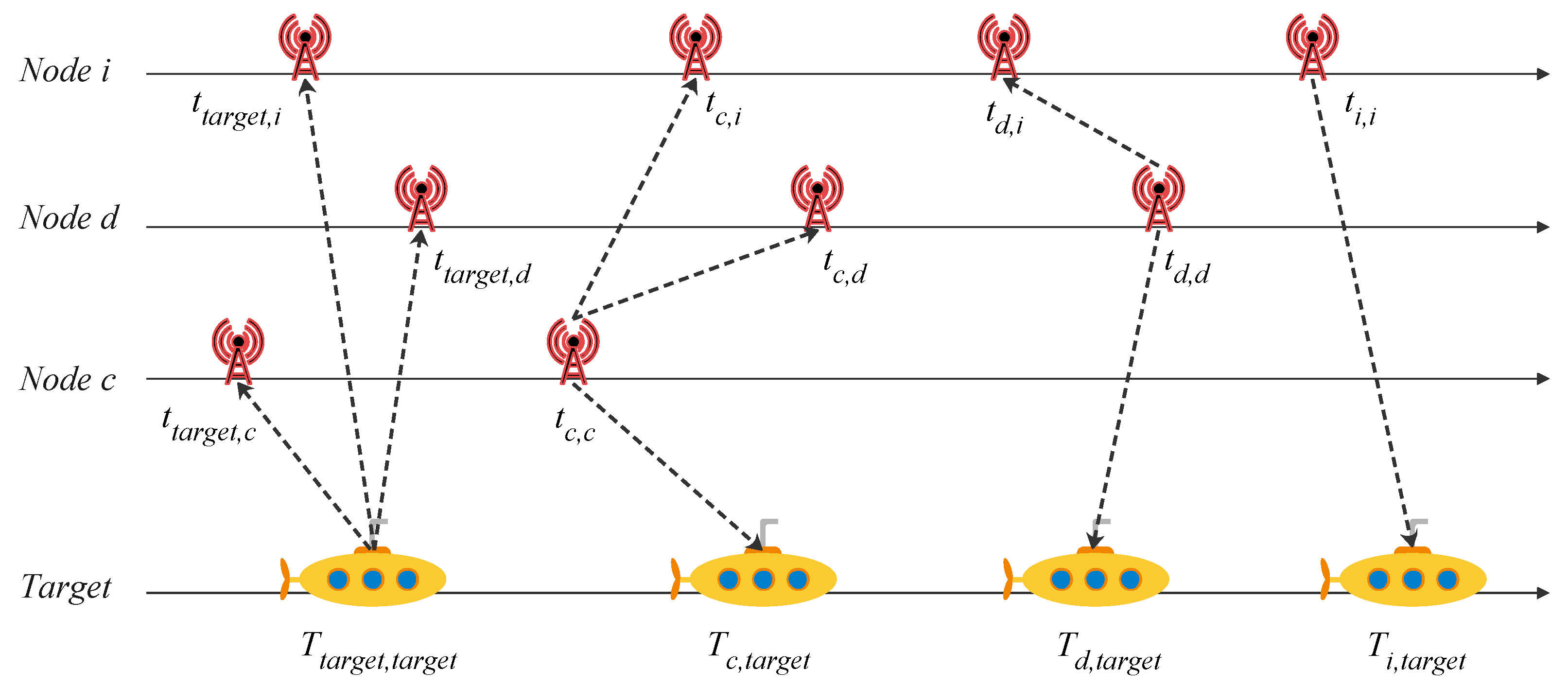
The active sensor node a sends out the detection signal. After hitting the target, the detection signal is reflected and received by other surrounding sensor nodes, such as sensor node c. The network completes the target detection through signal analysis. Here, we use a simple two-dimensional schematic Figure 2 to describe. The constant velocity vector of the target in a certain period of time $t\in \left[0,t_{slot}\right]$ is $V_{target}={\left(v_{xtarget},v_{ytarget}\right)}^T$, and its velocity relative to sensor nodes a and c are $V_a$ and $V_b$, respectively. It is known that the coordinate of sensor node a is $Lo{c}_a={\left(x_a,y_a\right)}^T$, and the coordinate of sensor node c is $Lo{c}_c={\left(x_c,y_c\right)}^T$.

The detection signal $Q_{sen}$ sent by sensor node a is:

$$Q_{sen}\left(t\right)=A{e}^{j\left(2\pi fr{e}_{0}t+k\pi t^2\right)},t\in \left[0,t_{slot}\right]$$

(1)

where the vibration amplitude of the signal is A, $fr{e}_0$ represents the initial frequency of the signal, and k is a constant. Accordingly, the reflected signal $Q_{rec}$ received by the sensor node c:

$$Q_{rec}\left(t\right)=\rho Q_{sen}\left(\beta \left(t-\chi \right)\right)=\rho A{e}^{j\left(2\pi fr{e}_0\beta \left(t-\chi \right)+k\pi {\beta }^2{\left(t-\chi \right)}^2\right)}$$

(2)

Here, $\rho$ refers to the propagation loss index. The Doppler shift is represented by $\beta$, and $\chi$ is the communication delay. The average velocity scalar of underwater acoustic signal is $v_{ocean}$, and the Doppler frequency shift $\beta$:

$$\beta =\left(v_{ocean}-v_a\right)/\left(v_{ocean}+v_c\right)$$

(3)

The coordinates of the target are expressed as $Lo{c}_{target}={\left(x_{target},y_{target}\right)}^T$, and the velocity $v_{target}=∥V_{target}∥$ at time $t=0$ is:

$$\left\{\begin{array}{c}\begin{array}{c}{v}_a={\left(Lo{c}_{target}-Lo{c}_a\right)}^T{V}_{target}/∥Lo{c}_{target}-Lo{c}_a∥\end{array}\\ v_c={\left(Lo{c}_{target}-Lo{c}_c\right)}^T{V}_{target}/∥Lo{c}_{target}-Lo{c}_c∥\end{array}\right.$$

(4)

Suppose $v_a$ does not change during the time from the detection signal sending out $t=0$ to the detection signal reaching the target $t={\chi }_0$, where the arrival time is ${\chi }_0=∥Lo{c}_{target}-Lo{c}_a∥/\left(v_{ocean}-v_a\right)$. The position of the target has changed in this time period, and the changed position is calculated as $Lo{c}_{{\chi }_{0}target}=Lo{c}_{target}+V_{target}{\chi }_0$. The relationship between time delay, sensor coordinates, and target coordinates can be obtained:

$$∥Lo{c}_a-Lo{c}_{{\chi }_{0}target}∥+∥Lo{c}_c-Lo{c}_{{\chi }_{0}target}∥=v_{ocean}\chi$$

(5)

The maximum effective distance of detection signal is set as $R_{max}$. The maximum delay ${\chi }_{max}=2R_{max}/v_{ocean}$ can be obtained. Then, within the time range $t\in \left[{\chi }_{max},t_{slot}\right]$, after the receiver signal described in (2) passes through the low-pass filter, the form is similar to (1), which can be expressed as:

$$Q_{rec}\left(t\right)=A_{rec}{e}^{j\left(2\pi {\widetilde{fre}}_{0}t+\pi \tilde{k}{t}^2+\omega \right)}$$

(6)

The estimated value of the initial frequency is ${\widetilde{fre}}_0=fr{e}_0\left(1-\beta \right)+k{\beta }^2\chi$ and the estimated value of the constant is $\tilde{k}=k\left(1-{\beta }^2\right)$. Here, $A_{rec}$ is the vibration amplitude of the signal. The last $\omega$ is the phase delay, which has no impact on the detection and positioning results. In this way, the form of (6) conforms to the expression of the detection signal, ${\widetilde{fre}}_0$ and $\tilde{k}$ can be regarded as its initial frequency and frequency rate, respectively.

Finally, the state vector of the detection target is expressed as ${\mathrm{X}}_{target}=\left[x_{target},v_{xtarget},\right.$$\left.y_{target},v_{ytarget}\right]$. The state transition function $H\left(•\right)$ in this paper is nonlinear. The additive process noise is $\delta \left(•\right)$. The state formula at time is as follows:

$$\mathrm{X}\left(t\right)=H\left(\mathrm{X}\left(t-1\right),\delta \left(t\right)\right)$$

(7)

(3)

Propagation Model

The clocks of underwater sensor nodes and targets are asynchronous. At the real-time t, the clock model established on the target is:

$$T_{target}=\mu t+\epsilon$$

(8)

where $\mu$ is clock pulse phase difference, and $\epsilon$ is the offset of the target relative to the real-time clock. According to the previous paper [35], the impulse channel response $Rp\left(t\right)$ of time t is as follows:

$$Rp\left(t\right)={\sum }_{t=0}^{P-1}{A}_p\left(t\right)\delta \left(t-{\chi }_p+{\beta }_{p}t\right)$$

(9)

where P represents the total number of signal transmission paths. In path p, the amplitude and delay are expressed as $A_p$ and ${\chi }_p$, respectively, and the corresponding Doppler frequency is represented by ${\beta }_p$. When the transmission distance and reception distance are l km and $l_{rec}$ km, respectively, the reception intensity of the acoustic signal at the frequency of $fre$ Hz is $S_{rec}\left(l,fre\right)$:

$$S_{rec}\left(l,fre\right)=S_{sen}-10\rho lg\left(l/l_{rec}\right)-b\left(fre\right)\left(l-l_{rec}\right)$$

(10)

where the subtracted $S_{sen}$ is the transmitted signal strength, and $\rho$ is the path loss index in the transmission process. The absorption coefficient is expressed as b, which is correlated with the frequency of the signal.

(4)

Energy Model

According to the description in the previous paper [36], the communication energy consumption $E{n}_{tr}$ in signal transmission depends on the packet bit length B and the transmission distance l:

$$E{n}_{tr}\left(B,l\right)=BE{n}_{re}+4.2\times {10}^{-9.5}B{t}_{tr}D{e}^{b\left(fre\right)l}$$

(11)

where $BE{n}_{re}$ represents the energy required by the sensor node to receive the B bit length signal. The time consumed in the transmission process is $t_{tr}$. D represents the depth of the sensor node. The sensor node knows that $E{n}_{ini}$ is its initial total energy, and its residual energy $E{n}_{rem}$ can be obtained from the following formula:

$$E{n}_{rem}=E{n}_{ini}-\left(E{n}_{tr}+BE{n}_{re}\right)$$

(12)

(5)

Overview of ST-BPN

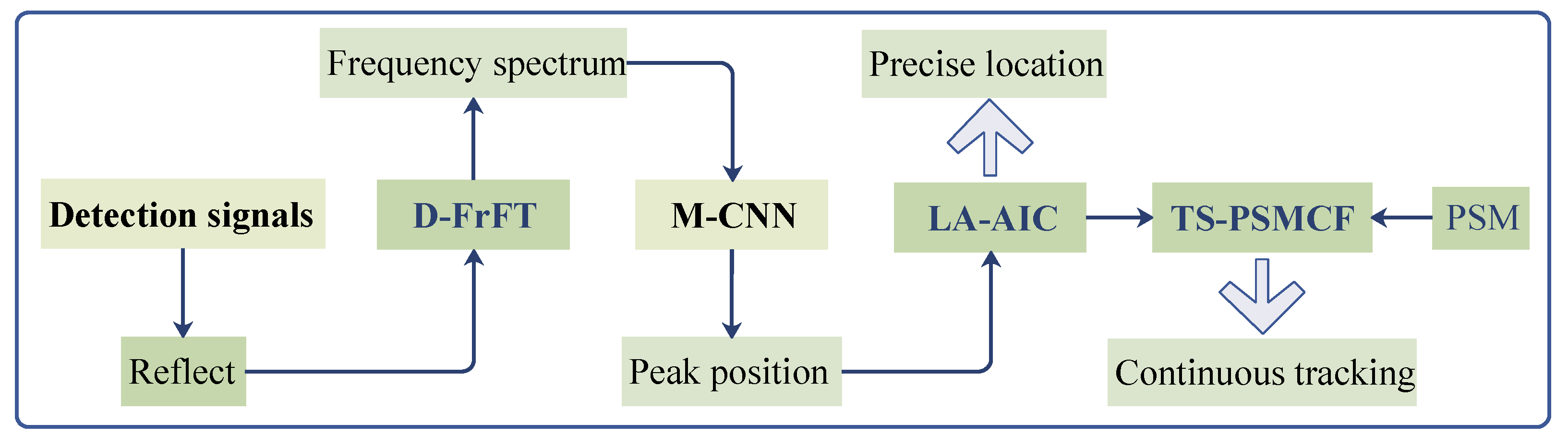
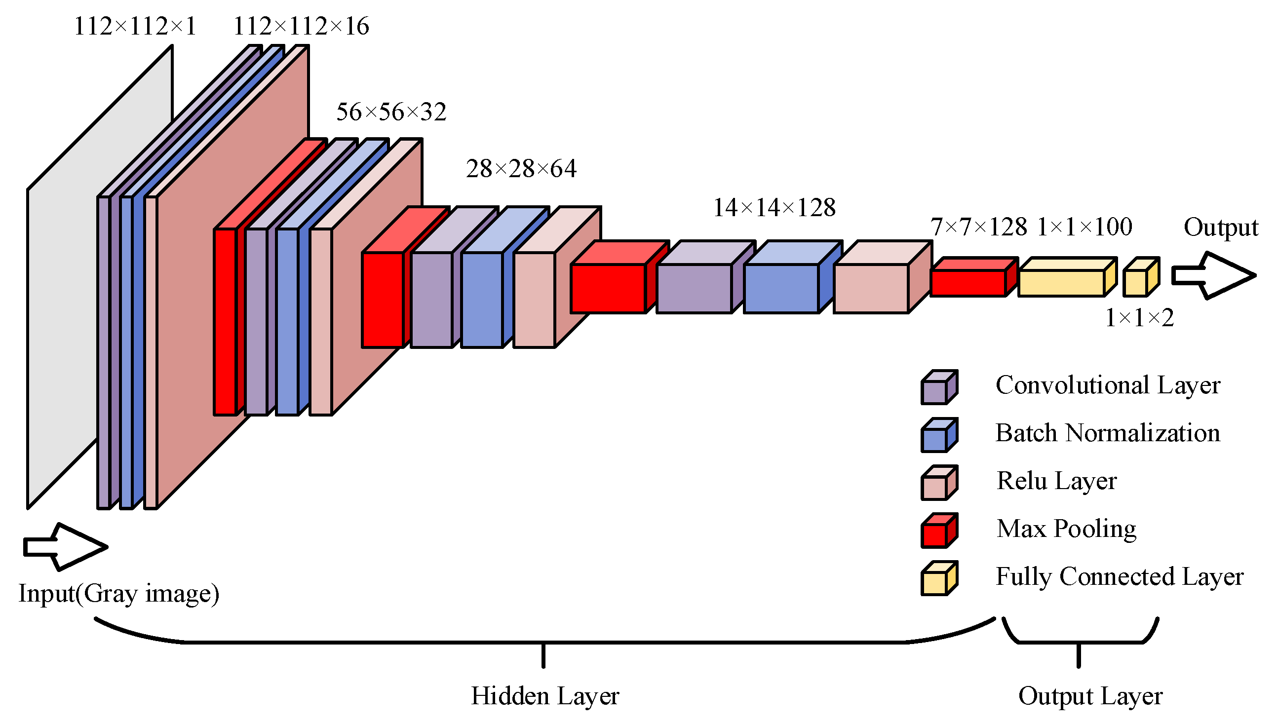
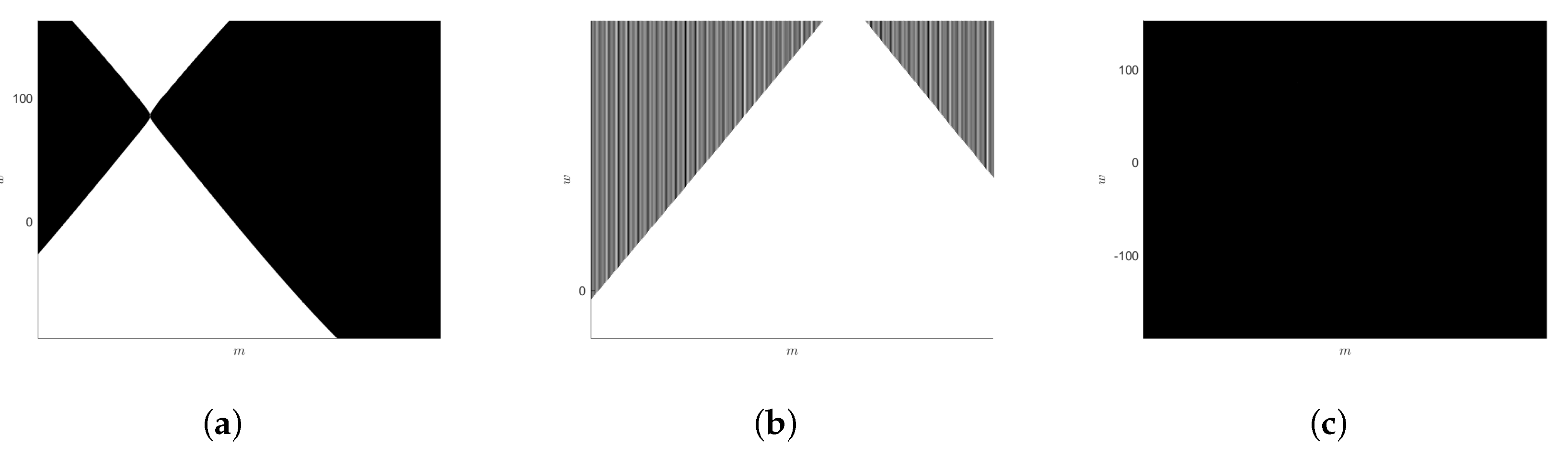
Figure 3 shows the overall process of ST-BPN. Throughout ST-BPN, UWSN is an active detection network. Active sensor nodes broadcast detection signals periodically, and the detection signals will be reflected when they touch the target object. Therefore, D-FrFT is used for signal analysis to extract frequency spectrum information. M-CNN is built to search the peak. After the peak of the frequency spectrum is searched by M-CNN, the LA-AIC is designed for localization based on the rough estimation position. The target is not stationary, and it will continue to move. Therefore, TS-PSMCF is proposed to complete the task of continuous tracking of the target. TS-PSMCF combines the weighted consensus algorithm with the principle of Bayesian filtering. Moreover, PSM is added to TS-PSMCF. The main idea of PSM is to predict the motion trajectory of the target, the nodes that meet the working conditions are awakened to track the target, and other nodes are in standby state.

3. Search and Locate Underwater Targets

In the process of analyzing the reflected signal, we aimed at the problems of low parameter estimation accuracy, large amounts of calculation, and non-clock synchronization. M-CNN is built to preliminarily detect the target. LA-AIC is used to locate the target.

3.1. M-CNN

(1)

Problem Formulation

To solve the problem of how to identify the target, a simple method is to set a threshold. When the spectrum value is higher than the threshold, it is proved that the target exists. However, the frequency spectrum of the reflected signal shown in Figure 4 is not a simple sparse state. Even if the size of the target is huge and the number of target is 1, there will be many local peaks in the frequency spectrum, and some local peaks are almost the same as the global peak. Moreover, UWSNs in practical application cannot only face a single target. With the uncertainty of the number of targets, the analysis of frequency spectrum will become more complex. Next, the traditional processing method of reflected detection signal is briefly described and analyzed:

In the development of UWSNs in recent years, fractional Fourier transform (FrFT) is a classical underwater acoustic signal processing method. Fortunately, a fast discrete fractional Fourier transform (D-FrFT) algorithm is proposed. As shown in Figure 4, it is a simulation case of the D-FrFT. The basic parameters are set as follows: sampling rate of 400 Hz, initial frequency of 120 Hz and initial frequency rate of 4.2 Hz/s.

In UWSNs, sensor node a periodically broadcasts the detection signal, and the detection model is described above. The node c receiving the reflected signal obtains the radial velocity of the target relative to it, as shown in (4). The reflected signal is described by (6). Estimations of initial frequency and frequency rate were obtained by D-FrFT. If the number of nodes receiving the reflected signal is $NUM$, $2NUM$ equation can be obtained. Combining these $2NUM$ equations, the least square algorithm is used to estimate the target position and radial velocity.

(2)

Motivation

From the analysis of the above traditional D-FrFT method and Figure 4 with complex lines, it is not difficult to see that the calculation cost is relatively high. Another important problem is how to accurately locate the peak. Moreover, the localization problem depends on the size of the sampling interval. If the sampling interval is blindly reduced, it will bring huge computational load. In order to solve the problems of high computational cost and low peak location accuracy, this paper establishes the M-CNN scheme, and solves the above two problems at the same time. The use of M-CNN only needs a rough spectrum to accurately identify the required patterns.

Figure 5 is a top gray image near the peak of Figure 4. The shape of this part is very similar to the hourglass in daily life. Here, it is called “hourglass” image mode. The position and width of this “hourglass” mode change with the parameters, but it is worth noting that even if the spectrum acquisition rate is very low, the “hourglass” mode is still obvious and will not disappear or be unrecognized. To sum up, we can obtain the frequency spectrum by under-sampling, which plays a role in saving energy consumption. Next, the “hourglass” mode is searched on the frequency spectrum. The search method adopts M-CNN, which improves the search accuracy. In this way, high location accuracy can be obtained under low complexity.

(3)

M-CNN

Figure 6 is the structure of M-CNN. The input is the gray image obtained by processing the spectral map of the reflected signal. The pixels of the grayscale image are $112\times 112$. The scale of the image input section is expressed as $112\times 112\times 1$. There are only two output results of M-CNN—one is “positive” and the other is “negative”. The output result is related to whether the input image can be recognized.

The structure of CNN is divided according to the number of convolution layers. In this paper, M-CNN is divided into four layers, and the basic composition of each layer is the same. Each layer includes convolution layer, batch normalization layer, Relu layer and maximum pooling layer. The main work of convolution layer is to extract the features in gray image, and the features to be extracted are “hourglass” pattern. The setting of batch normalization layer can accelerate the convergence rate, improve the generalization ability of the network, disrupt the order when training data, reduce the probability that a picture is repeatedly selected, improve the diversity of training, and improve the accuracy of network recognition. The Relu layer retains the values with good characteristics and rounds off the bad values. The function of the maximum pool layer can be seen from the Figure 6, that is to greatly reduce the order of parameters and avoid over fitting, that is, compress the image. Two fully connected layers are set in the output layer, and their main function is classification.

After M-CNN is set up, it will begin to train it. The first is the preparation of training set. The simulation software is used to generate different frequency spectra under different parameters, and the gray image is divided into several small blocks. Figure 7 shows three cases of segmented small image. Figure 7a is an example of an image output as “positive”, and the “hourglass” mode in the figure is clearly visible. Figure 7b,c are two examples of images whose output is “negative”. These two images feedback completely different information to M-CNN. Figure 7c is all black and there is only noise. Figure 7b is taken from a part of the “hourglass” image, and it is inferred that it is possible to obtain a complete “hourglass” mode by moving the window up.

After the data set required for basic training is prepared, the quantity and type of data are still insufficient. Here, the data enhancement technology is introduced, and the processing methods include gray adjustment, horizontal/vertical flipping, angle conversion, and size adjustment of the existing image. The program automatically divides the spectrum into multiple small blocks, and each small block is saved as an image in PNG format. There are two folders for saving images, one named “YES” and the other named “NO”. The application of data enhancement technology is also mainly aimed at the images in the folder “YES”. In order to distinguish them, different names are used. The specific training and experimental results are described in detail in the sixth part of this paper.

3.2. LA-AIC

If we want to improve the accuracy of the estimated position, we need to consider the problem of underwater clock. This paper proposes LA-AIC, which can resist the influence of clock asynchrony. The number of nodes that can receive the reflected signal is $NUM$, and every three nodes form a “localization combination”. The most important information provided by the localization combination is the time stamp. Take out a localization combination arbitrarily, and the three nodes are $c\left(x_c,y_c,z_c\right)$, $d\left(x_d,y_d,z_d\right)$, and $i\left(x_i,y_i,z_i\right)$, respectively. The propagation process of localization information is shown in Figure 8, which is described as follows:

(1)

The time when the detection signal is reflected by the target is recorded as $T_{target,target}$. Other sensor nodes float around the target. These nodes can receive reflected signals. Sensor nodes c, d, and i receive signals and record the receiving times as $t_{target,c}$, $t_{target,d}$, and $t_{target,i}$, respectively.

(2)

The sensor nodes c, d, and i receive the signal turn on the locaization mode of the target, which constitutes a localization combination. Each member of the localization group begins to send the information needed to locate the target to the network. The localization information structure is shown in Figure 9.

(3)

The time when the target receives the positioning information of the sensor node is recorded as $T_{c,target}$, $T_{target,d}$, and $T_{target,i}$, respectively. In this way, the information interaction of a group of localization units is completed. The following is using this known information to locate the target:

Now, the most important thing is to solve the problem of clock asynchrony. In (8), the clock model of the target is established. The model contains two important parameters: $\mu$ and $\epsilon$. If we can eliminate their influence, the localization process will no longer be disturbed by the asynchronous clock. Firstly, the relationship between different timestamps is established as follows:

$$\left\{\begin{array}{c}\begin{array}{c}\begin{array}{c}{\zeta }_{c,d}=\left(t_{c,d}-t_{target,d}\right)-\left(t_{c,c}-t_{target,c}\right)={\chi }_{target,c}+{\chi }_{c,d}-{\chi }_{target,d}+{\eta }_{c,d}\\ {\zeta }_{c,i}=\left(t_{c,i}-t_{target,i}\right)-\left(t_{c,c}-t_{target,c}\right)={\chi }_{target,c}+{\chi }_{c,i}-{\chi }_{target,i}+{\eta }_{c,i}\end{array}\\ {\zeta }_{d,c}=t_{target,d}-t_{target,c}={\chi }_{target,d}-{\chi }_{target,c}+{\eta }_{d,c}\end{array}\\ {\zeta }_{d,i}=\left(t_{d,i}-t_{target,i}\right)-\left(t_{d,d}-t_{target,d}\right)={\chi }_{target,d}+{\chi }_{d,i}-{\chi }_{target,,i}+{\eta }_{d,i}\\ {\zeta }_{i,c}=t_{target,i}-t_{target,c}={\chi }_{target,i}-{\chi }_{target,c}+{\eta }_{i,c}\\ {\zeta }_{i,d}=t_{target,i}-t_{target,d}={\chi }_{target,i}-{\chi }_{target,d}+{\eta }_{i,d}\end{array}\right.$$

(13)

where $\chi$ refers to propagation delay, but here refers to unidirectional propagation delay. The specific calculation methods are ${\chi }_{target,j}=\left[{\left(x_{target}-x_j\right)}^2+{\left(y_{target}-y_j\right)}^2\right.$ ${\left.+{\left(z_{target}-z_j\right)}^2\right]}^{1/2}/v_{ocean}$, ${\chi }_{m,j}={\left[{\left(x_m-x_j\right)}^2+{\left(y_m-y_j\right)}^2+{\left(z_m-z_j\right)}^2\right]}^{1/2}/v_{ocean}$ and $\left(m,j\in c,d,i,m\ne j\right)$. At the end of each formula, there is a measurement noise $\eta$. It is assumed that the measurement capability of each sensor node is the same. The measurement noise follows the zero mean Gaussian distribution and their variance is uniformly set to $\upsilon a{r}^2$. By substituting the calculation formula of propagation delay $\chi$ and $v_{ocean}$ = 1500 m/sinto (13), the relationship between coordinate position and propagation delay can be constructed:

$$\underset{:=\psi }{\underbrace{\left[\begin{array}{c}{v}_{ocean}{\zeta }_{c,d}\hfill \\ v_{ocean}{\zeta }_{c,i}\hfill \\ v_{ocean}{\zeta }_{d,c}\hfill \\ v_{ocean}{\zeta }_{d,i}\hfill \\ v_{ocean}{\zeta }_{i,c}\hfill \\ v_{ocean}{\zeta }_{i,d}\hfill \end{array}\right]}}=\underset{:=\hslash }{\underbrace{\left[\begin{array}{c}{l}_{target,c}+l_{c,d}-l_{target,d}\hfill \\ l_{target,c}+l_{c,i}-l_{target,i}\hfill \\ l_{target,d}-l_{target,c}\hfill \\ l_{target,d}+l_{d,i}-l_{target,,i}\hfill \\ l_{target,i}-l_{target,c}\hfill \\ l_{target,i}-l_{target,d}\hfill \end{array}\right]}}+\underset{:=\lambda }{\underbrace{\left[\begin{array}{c}{v}_{ocean}{\eta }_{c,d}\hfill \\ v_{ocean}{\eta }_{c,i}\hfill \\ v_{ocean}{\eta }_{d,c}\hfill \\ v_{ocean}{\eta }_{d,i}\hfill \\ v_{ocean}{\eta }_{i,c}\hfill \\ v_{ocean}{\eta }_{i,d}\hfill \end{array}\right]}}$$

(14)

where l represents the relative distance, and the calculation formula are $l_{target,j}=\left[\left(x_{target}\right.\right.$${\left.{\left.-x_j\right)}^2+{\left(y_{target}-y_j\right)}^2+{\left(z_{target}-z_j\right)}^2\right]}^{1/2}$, $l_{m,j}={\left[{\left(x_m-x_j\right)}^2+{\left(y_m-y_j\right)}^2+{\left(z_m-z_j\right)}^2\right]}^{1/2}$ and $\left(m,j\in c,d,i,m\ne j\right)$. After constructing formula $\psi =\hslash +\lambda$, its Jacobian matrix can be calculated as follows:

$$Jac=\left[\begin{array}{c}\begin{array}{cc}\frac{x_{target}-x_c}{l_{target,c}}-\frac{x_{target}-x_d}{l_{target,d}}& \frac{y_{target}-y_c}{l_{target,c}}-\frac{x_{target}-y_d}{l_{target,d}}\end{array}\hfill \\ \begin{array}{cc}\frac{x_{target}-x_c}{l_{target,c}}-\frac{x_{target}-x_i}{l_{target,i}}& \frac{x_{target}-x_c}{l_{target,c}}-\frac{x_{target}-x_i}{l_{target,i}}\end{array}\hfill \\ \begin{array}{cc}\frac{x_{target}-x_d}{l_{target,d}}-\frac{x_{target}-x_c}{l_{target,c}}& \frac{y_{target}-y_d}{l_{target,d}}-\frac{x_{target}-y_c}{l_{target,c}}\end{array}\hfill \\ \begin{array}{cc}\begin{array}{c}\frac{x_{target}-x_d}{l_{target,d}}-\frac{x_{target}-x_i}{l_{target,i}}\hfill \\ \frac{x_{target}-x_i}{l_{target,i}}-\frac{x_{target}-x_c}{l_{target,c}}\hfill \\ \frac{x_{target}-x_i}{l_{target,i}}-\frac{x_{target}-x_d}{l_{target,d}}\hfill \end{array}& \begin{array}{c}\frac{y_{target}-y_d}{l_{target,d}}-\frac{x_{target}-y_i}{l_{target,i}}\hfill \\ \frac{y_{target}-y_i}{l_{target,i}}-\frac{x_{target}-y_c}{l_{target,c}}\hfill \\ \frac{y_{target}-y_i}{l_{target,i}}-\frac{x_{target}-y_d}{l_{target,d}}\hfill \end{array}\end{array}\hfill \end{array}\right]$$

(15)

Here, we can get a least squares estimator $\left[{\widehat{x}}_{target}\left(k+1\right),{\widehat{y}}_{target}\left(k+1\right)\right]=\left[{\widehat{x}}_{target}\left(k\right),\right.$$\left.{\widehat{y}}_{target}\left(k\right)\right]-{\left[Ja{r}^{T}Jar\right]}^{-1}Ja{r}^T\varpi$. where k represents the iteration step. $\varpi =\left[\psi \left(1\right)-\hslash \left(1\right),\right.$${\left.\psi \left(2\right)-\hslash \left(2\right),\psi \left(3\right)-\hslash \left(3\right),\psi \left(4\right)-\hslash \left(4\right),\psi \left(5\right)-\hslash \left(5\right),\psi \left(6\right)-\hslash \left(6\right)\right]}^{{}^T}$ represents the error vector of the measurement equation.

4. Track Underwater Targets

The target is not fixed. How to realize the continuous tracking of the target has become a research problem. It is worth mentioning that the power supply mode of sensor nodes is the storage battery, and the total amount of battery energy is limited. Therefore, while realizing continuous target tracking, the control of energy consumption is also necessary. Aiming at the above problems, this paper proposes a tracking scheme based on consensus filtering of TS-PSMCF.

4.1. TS-PSMCF

TS-PSMCF is proposed, which assigns reasonable weights to each estimate mainly, and finally calculates the probability density function (PDF) of the target. The update of PDF also depends on the weight distribution of multiple groups of measurement data. Compared with the traditional Kalman filter tracking, TS-PSMCF (Algorithm 1) has obvious advantages, that is, it does not need to approximate the model in the iterative update process. The measurement equation can be constructed according to (14) and (15):

$$\begin{array}{c}{\mathrm{Z}}_s\left(k\right)=Y_s\left(\widehat{\mathrm{X}}\left(k\right)\right)=v_{ocean}{\left[{\zeta }_{c,d},{\zeta }_{c,i},{\zeta }_{d,c},{\zeta }_{d,i},{\zeta }_{i,c},{\zeta }_{i,d}\right]}^T\\ =\underset{Y_s\left(\mathrm{X}\left(k\right)\right)}{\underbrace{v_{ocean}\left[\begin{array}{c}{\chi }_{target,c}+{\chi }_{c,d}-{\chi }_{target,d}\hfill \\ {\chi }_{target,c}+{\chi }_{c,i}-{\chi }_{target,i}\hfill \\ {\chi }_{target,d}-{\chi }_{target,c}\hfill \\ {\chi }_{target,d}+{\chi }_{d,i}-{\chi }_{target,,i}\hfill \\ {\chi }_{target,i}-{\chi }_{target,c}\hfill \\ {\chi }_{target,i}-{\chi }_{target,d}\hfill \end{array}\right]}}+\underset{{\varsigma }_s\left(k\right)}{\underbrace{v_{ocean}\left[\begin{array}{c}{\eta }_{c,d}\hfill \\ {\eta }_{c,i}\hfill \\ {\eta }_{d,c}\hfill \\ {\eta }_{d,i}\hfill \\ {\eta }_{i,c}\hfill \\ {\eta }_{i,d}\hfill \end{array}\right]}}\end{array}$$

(16)

The total number of sensor nodes that can receive signals is $NUM$, and the number of location units that can be formed is $N_{LU}=NUM\left(NUM-1\right)\left(NUM-2\right)/6$ and $\left(N_{LU}>1\right)$. The subscript s in the observation equation refers to one of the location units. The total measured value can be expressed as $Z\left(k\right)=\left[Z_1\left(k\right),Z_2\left(k\right),...,Z_{N_{LU}}\left(k\right)\right]$, and the posteriori estimate we need is $P_s\left(\widehat{\mathrm{X}}\left(k\right)|Z_s\left(k\right)\right)$.

Algorithm 1: TS-PSMCF.

(1)

Initialization

The monitoring area of UWSN is $Area$, the iteration step is recorded as k, and the value of k in the initialization phase is 0. At first, the PDF $P_s\left(\widehat{\mathrm{X}}\left(0\right)|Z_s\left(0\right)\right)$ is evenly distributed over $Area$. Accordingly, the value of the PDF can be obtained as $P_s\left(\widehat{\mathrm{X}}\left(0\right)|Z_s\left(0\right)\right)=1/\left|Area\right|$, where $\left|Area\right|$ refers to the volume of the monitoring area.

(2)

Prediction

In the location unit s, the state transition probability is $P_s\left(\widehat{\mathrm{X}}\left(k\right)|\widehat{\mathrm{X}}\left(k-1\right)\right)$ and the measurement of the monitoring area is $A_{mea}\left(•\right)$, then the priori PDF of $\widehat{\mathrm{X}}\left(k\right)$ can be predicted in one step according to the following formula [37]:

$$\begin{array}{c}{P}_s\left(\widehat{\mathrm{X}}\left(k\right)|Z_s\left(k-1\right)\right)\hfill \\ ={\int }_{Area}{P}_s\left(\widehat{\mathrm{X}}\left(k\right)|\widehat{\mathrm{X}}\left(k-1\right)\right)P_s\left(\widehat{\mathrm{X}}\left(k-1\right)|Z_s\left(k-1\right)\right)d{A}_{mea}\left(\widehat{\mathrm{X}}\left(k-1\right)\right)\hfill \end{array}$$

(17)

(3)

Update

Based on the predicted value of (17) and the principle of Bayesian filtering [38], the posterior PDF calculation formula in positioning unit s is:

$$\left\{\begin{array}{c}{P}_s\left(\widehat{\mathrm{X}}\left(k\right)|Z_s\left(k\right)\right)=U\left(Z_s\left(k\right)|\widehat{\mathrm{X}}\left(k\right)\right)P_s\left(\widehat{\mathrm{X}}\left(k\right)|Z_s\left(k-1\right)\right)/\phantom{U\left(Z_s\left(k\right)|\widehat{\mathrm{X}}\left(k\right)\right)P_s\left(\widehat{\mathrm{X}}\left(k\right)|Z_s\left(k-1\right)\right)P_s\left(Z_s\left(k\right)|Z_s\left(k-1\right)\right)}{P}_s\left(Z_s\left(k\right)|Z_s\left(k-1\right)\right)\hfill \\ P_s\left(Z_s\left(k\right)|Z_s\left(k-1\right)\right)={\int }_{Area}U\left(Z_s\left(k\right)|\widehat{\mathrm{X}}\left(k\right)\right)P_s\left(\widehat{\mathrm{X}}\left(k\right)|Z_s\left(k-1\right)\right)d{A}_{mea}\left(\widehat{\mathrm{X}}\left(k-1\right)\right)\hfill \end{array}\right.$$

(18)

Then, decompose the likelihood function $U\left(Z_s\left(k\right)|\widehat{\mathrm{X}}\left(k\right)\right)$ in the above formula:

$$U\left(Z_s\left(k\right)|\widehat{\mathrm{X}}\left(k\right)\right)=C\left(Z_s\left(k\right)|\widehat{\mathrm{X}}\left(k\right)\right){\prod }_{i\in {\xi }_s^{*}}C\left(Z_s\left(k\right)|\widehat{\mathrm{X}}\left(k\right)\right)$$

(19)

where $C\left(Z_s\left(k\right)|\widehat{\mathrm{X}}\left(k\right)\right)$ is the conditional PDF of $\widehat{\mathrm{X}}\left(k\right)$, here ${\xi }_s^{*}={\xi }_s\cup \left\{s\right\}$.

(4)

Fusion based on consensus filter

Firstly, it should be pointed out that the iteration here refers to the iteration between different localization units, and the number of iterations is set to $\kappa =0,1,...,{\kappa }_{end}$. For each iteration, the weighted consistency scheme is applied [39]:

$$P_s^{\kappa +1}\left(\widehat{\mathrm{X}}\left(k\right)|Z_s\left(k\right)\right)={\sum }_{j\in {\xi }_s^{*}}{\omega }_{j,s}\left(k\right)P_s^{\kappa }\left(\widehat{\mathrm{X}}\left(k\right)|Z_s\left(k\right)\right)$$

(20)

where ${\omega }_{j,i}$ is the weight between localization unit j and location unit s, and its value range is ${\omega }_{j,s}\ge 0$. When the iteration is completed, the value of $P_s^{{\kappa }_{end}+1}\left(\widehat{\mathrm{X}}\left(k\right)|Z_s\left(k\right)\right)$ can be obtained.

(5)

Estimation

The estimated location information is closely related to the PDF involved in the previous four steps, then the estimation of $\widehat{\mathrm{X}}\left(k\right)$ can be calculated:

$$P_s\left(\widehat{\mathrm{X}}\left(k\right)|Z_s\left(k\right)\right)=P_s^{{\kappa }_{end}+1}\left(\widehat{\mathrm{X}}\left(k\right)|Z_s\left(k\right)\right)$$

(21)

On the basis of Bayesian filtering without fusion link, TS-PSMCF introduces the process of weight allocation to the traditional consensus algorithm, and then combines the two by using the fusion step, so as to achieve the result that the estimated value tends to the overall optimal, which undoubtedly improves the accuracy in the tracking process.

4.2. PSM

The total battery energy of sensor nodes is limited. Usually, the battery is not replaceable or rechargeable. In order to save energy consumption, PSM is added in the implementation of TS-PSMCF. PSM divides the states of each sensor node into two types, one is the awakened working state and the other is the dormant standby state. The energy consumption of nodes in dormant standby state is very low and almost negligible. Only the nodes that meet the working conditions will be switched to the wake-up working state by PSM, so as to achieve the purpose of energy saving. The schematic of PSM is shown in Figure 10.

Firstly, the sensor nodes in UWSN need to measure the distance information. Only nodes that meet the requirements can be awakened. Here, there is still a localization unit s, which contains three nodes, c, d, and i, respectively, and their communication distance is L.

Then, the conditions for determining whether the node is awakened are:

$$\sqrt{{\left(x_j-{\widehat{x}}_{target}\left(k\right)\right)}^2+{\left(y_j-{\widehat{y}}_{target}\left(k\right)\right)}^2+{\left(z_j-z_{target}\left(k\right)\right)}^2}\le L,\left(j\in c,d,i\right)$$

(22)

The trajectory is predicted by the difference method [40]. Then, when the update period is $\iota$, the prediction speed is:

$${\widehat{v}}_{mtarget}\left(k\right)=\left({\widehat{m}}_{target}\left(k\right)-{\widehat{m}}_{target}\left(k-1\right)\right)/\iota ,\left(m\in x,y,z\right)$$

(23)

Combining (23) with the state equation of the target (7), it can be obtained that the prediction trajectory $\left({\widehat{x}}_{target}\left(k+k^{*}\right),{\widehat{y}}_{target}\left(k+k^{*}\right),z_{target}\left(k+k^{*}\right)\right)$ of time interval $\left[k,k+k^{*}\right]$ is:

$${\widehat{m}}_{target}\left(k+k^{*}\right)={\widehat{m}}_{target}\left(k\right)+k^{*}\iota {\widehat{v}}_{mtarget}\left(k\right),\left(m\in x,y,z\right)$$

(24)

5. Simulation

In order to verify the effectiveness of M-CNN, LA-AIC, and TS-PSMCF with PSM, simulation experiments are set up in this part.

(1)

Search underwater targets based on M-CNN

The initial frequency used in the experiment is 1 kHz, the detection signal has an initial frequency rate of 20 Hz/s, the scanning period is 8 s, the maximum scanning radius of 3 km, and the sampling rate is set to 400 Hz. There are two kinds of output results of M-CNN, which belong to the most common binary classifier. The confusion matrix is used to summarize the results of the classifier. For binary classification, it is essentially a $2\times 2$ table, which records the prediction results of the classifier. This paper adds training samples for experiments, which are 200, 500, 750, and 1000, respectively. According to this confusion matrix (

Table 1. Confusion matrix.

	Number of Training Samples
	200		500		750		1000
	Output		Output		Output		Output
Input	Positive	Negative	Positive	Negative	Positive	Negative	Positive	Negative
True	95	5	245	5	371	4	449	1
False	2	98	7	243	5	370	2	448
Acc	0.965		0.976		0.988		0.997
PPV	0.979		0.972		0.987		0.996
TPR	0.95		0.98		0.989		0.998

), the technical indexes of M-CNN built in this paper can be calculated. Technical indicators include network accuracy (ACC), positive predictive value (PPV), and true positive rate (TPR). Their respective calculation formulas are as follows:

$$\left\{\begin{array}{c}Acc=\left(TP+FN\right)/\left(TP+FN+TN+FP\right)\hfill \\ PPV=TP/\left(TP+FP\right)\hfill \\ TPR=TP/\left(TP+FN\right)\hfill \end{array}\right.$$

(25)

Table 1 contains the results of four groups of network training. The number of training samples are 200, 500, 750, and 1000, respectively. The input and output results are counted in Table 1, and the values of the three indicators are also added. It is not difficult to see from Table 1 that the calculated values of technical indicators are very considerable, and the values of the three indicators increase in turn with the increase of training samples. This shows the effectiveness of the M-CNN network built in this paper, which can identify the peak position accurately. M-CNN lays a solid foundation for the effective implementation of subsequent positioning algorithms and saves the computational overhead of sampling data, which can be described as killing two birds with one stone.

(2)

Simulation of LA-AIC

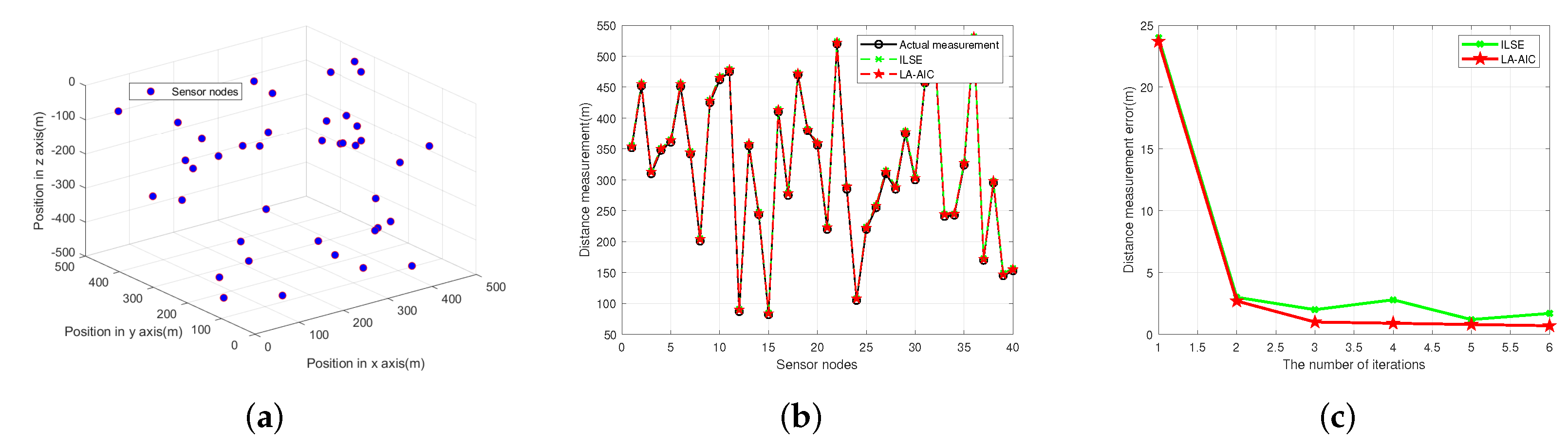
This paper assumes that all nodes can communicate effectively, regardless of unexpected situations such as connection interruption. Moreover, the data packets transmitted by communication can be normally received, decoded, and transmitted. As shown in Figure 11a, it is a three-dimensional display of the whole monitoring area $Area$, with a volume of 500 m × 500 m × 500 m. Among them, $Area$ includes 4 water surface sensors and 40 underwater sensor nodes. The length of the data packet is 2 bits. The initial energy of each node is 250 kJ, and its energy consumption for receiving information is 0.5 J. The number of times the cycle ends is 100. The initial frequency of the signal is set to 10 kHz. The update duration is 5 s. L in PSM is set to 200 m. Clock information $\mu =1.05\mathrm{s}$ and $\epsilon =0.01\mathrm{s}$. Finally, the noise setting is: $\upsilon a{r}^2=0.{001}^2$ and $\delta \sim N\left(0.1,0.01\right)$.

The most important purpose of LA-AIC experiment is to verify its applicability to clock asynchrony. Here, the iterative least squares method [41] is used in the final position determination scheme (ILSE) for comparison. This paper sets up two experimental scenarios. The differences between the two scenarios are derived from the parameters in (8). First, if the clock pulse phase difference $\mu$ in the clock model of the target object is ignored, the clock model of the target object is converted to $T_{target}=t+\epsilon$. Different from the first experimental scenario, the second one adds clock phase difference $\mu$ and clock offset $\epsilon$ into the target clock model. The main comparison in the experiment is the iterative error value.

Experimental data analysis of the first scenario:

Before the statistics of iterative error, the ranging data are analyzed. Figure 11b shows the ranging comparison of the first experimental scenario. It is not difficult to see that the ranging results of LA-AIC and ILSE are almost the same as the real values. They can complete accurate ranging tasks without considering the phase difference of clock pulses. Further, the iterative error is numerically counted to form two broken lines in Figure 11c. There is no obvious difference in change trend or numerical comparison. However, the error of ILSE is significantly higher than that of LA-AIC, especially in 4 iterations, where the maximum difference is 2 m. Therefore, it is concluded that both LA-AIC and ILSE can complete the distance measurement and target location without the influence of clock pulse phase difference.

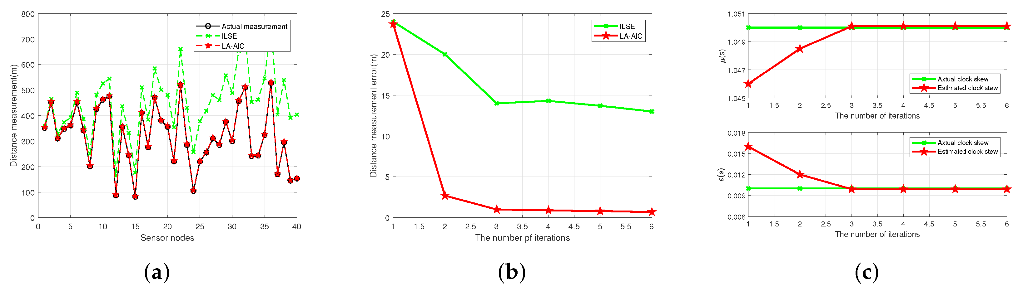
Experimental data analysis of the second scenario:

The situation in scenario 2 is more general, because the change speed of the clock depends on the phase difference of the clock pulse, so the phase difference of the clock pulse cannot be ignored in practice. Generally, the phase difference of clock pulse follows the normal distribution with the mean value of 1. In this paper, 1.05 is selected as its value. Like the first scenario, the data analysis of the second experimental scenario also uses the comparison of ranging data (Figure 12a) and the numerical comparison of iterative error (Figure 12b). In addition, the analysis of two additional clock information is added (Figure 12c). Firstly, according to the observation and analysis of Figure 12a, the broken line of ILSE tends to deviate from the real value with the increase of the number of sensor nodes. This is because the more the number of sensor nodes participating in the ranging task, the more obvious the cumulative effect of error will be. It should be noted that the broken line of LA-AIC is basically the same as that in Figure 11b, which is almost always close to the broken line of the real value without much deviation. This is because LA-AIC can effectively resist the influence of clock asynchrony. Even if the clock pulse phase difference and clock offset work together to interfere with ranging, LA-AIC can still complete the ranging task, which lays a solid foundation for subsequent location calculation tasks. Let us look at Figure 12b. The overall trend of the two broken lines decreases sharply in the first half and then tends to be flat. The broken line decrease is due to the increase of the number of iterations, which plays a role in adjusting the error. However, when the number of iterations exceeds a certain value, the impact of the number of iterations on the error is greatly weakened, and it can even be considered that the effect can be ignored. It can be seen from the figure that when the number of iterations reaches 3, the impact of the number of iterations on the two schemes is minimal. The error of ILSE is finally maintained between 13 m and 15 m, while the error of LA-AIC is 1 m to 2 m. This is because LA-AIC can effectively estimate the value of clock information. It will not be disturbed by clock synchronization. ILSE does not consider the problem of asynchronous clock, so it will be seriously disturbed. The error gap between ILSE and LA-AIC is about ten times, which fully proves that LA-AIC can resist the influence of clock synchronization and control sensor nodes to complete more accurate localization.

Here, the two clock information are clock pulse phase difference $\mu$ and clock offset $\epsilon$, which can be used to verify the practicability of the localization scheme. The values estimated by LA-AIC is compared with their real values, and Figure 12c is drawn as the analysis of the LA-AIC. The least square method is used to estimate the clock information. This estimation method is used in the clock information estimation of LA-AIC. In Figure 12c, the two estimated value polylines first tend to the real value with the increase of iterations. When the number of iterations exceeds a certain value, the polylines tend to remain unchanged and almost coincide with the real value curve. When the number of iterations reaches 3, the estimation results tend to converge. This indirectly proves the adaptability of LA-AIC to clock asynchrony. It can estimate the value of clock information effectively. Finally, it can eliminate the influence of clock and complete accurate localization.

(3)

Simulation of TS-PSMCF with PSM

The simulation experiment of TS-PSMCF scheme includes two important aspects. The first is the tracking error, and the energy consumption is the second aspect to be analyzed. Next, the performance of TS-PSMCF is plotted and analyzed from these two aspects.

Tracking error:

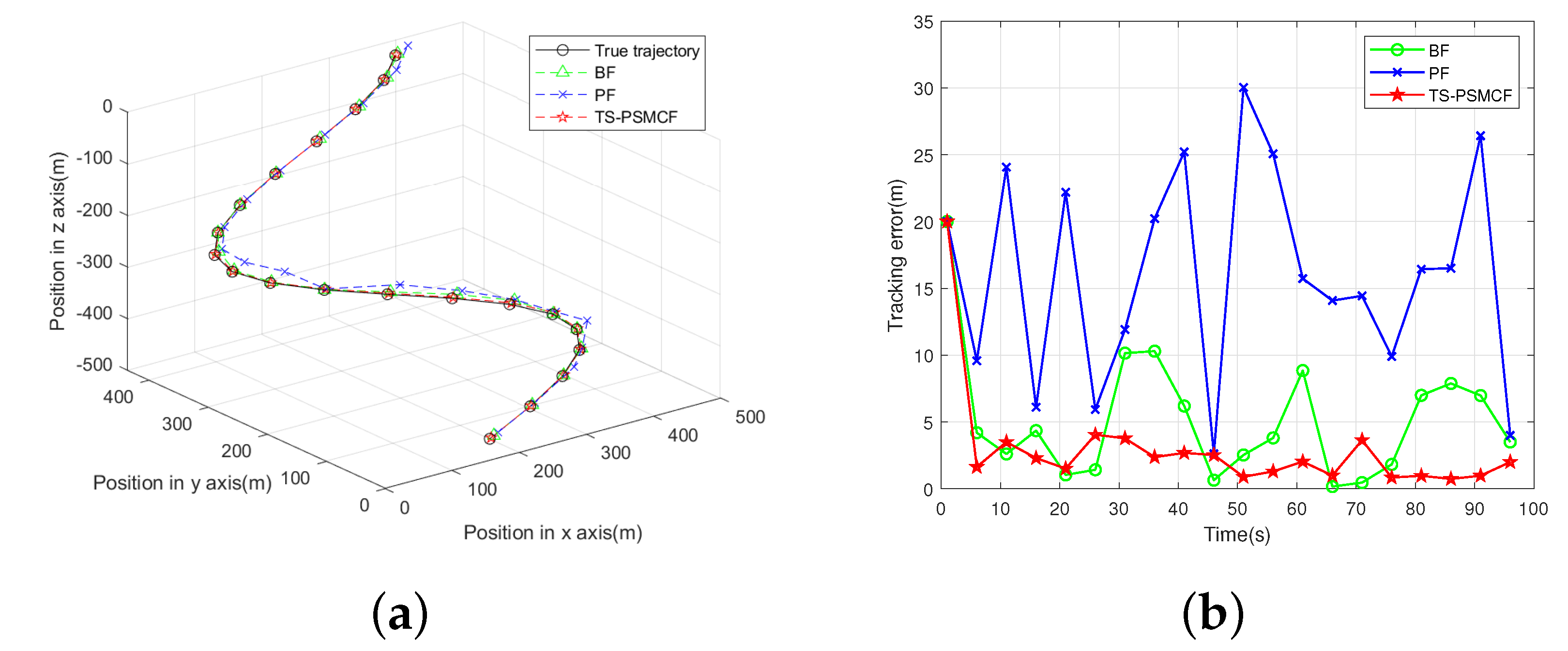
Other settings of the experimental scene refer to the previous paper [27], and the experimental part introduces the comparison group, which includes Bayesian filter tracking scheme (BF) [30] and particle filter scheme (PF) [42]. The comparison of tracking trajectories is shown in Figure 13a, and the error comparison corresponding to the trajectory diagram is drawn in Figure 13b. Looking at Figure 13a, the tracking curves of BF, PF, and TS-PSMCF can be regarded as tracking the target without unreasonable deviation. However, BF and PF have obvious trajectory deviation in some local areas, and TS-PSMCF tracking is the most stable and accurate of the three schemes. It is impossible to draw a very scientific conclusion by observing a three-dimensional tracking trajectory with the naked eye, and the error statistical comparison in Figure 13b is more convincing. The three error curves are ups and downs as a whole, but the range of ups and downs is obviously different. Here, the vibration amplitude of PF is the largest, and the vibration amplitude of TS-PSMCF is the smallest. The maximum error of PF is 30 m, which is unacceptable. The error value of TS-PSMCF is between 0 m and 5 m. With the passage of horizontal axis time, the broken lines of PF and BF do not show an obvious convergence trend, because there is no weighted consistency algorithm in PF to coordinate the overall situation, and there is no weight balance of fusion strategy and consistency algorithm in BF. The amplitude of TS-PSMCF decreases gradually, and finally shows an obvious convergence trend. It can be seen that with the global planning of weighted consistency algorithm and the blessing of fusion strategy, the classical Bayesian filtering algorithm shows the best tracking effect.

Energy consumption:

Before the graphical comparison of experimental data, several classical tracking algorithms are compared, and the comparison results are shown in

Table 2. Comparison of factors considered in classical tracking algorithms.

Reference	ILSE [41,43]	Single Source [28,44]	PF [42]	TS-PSMCF
$\mu$	◯	×	×	◯
$\epsilon$	×	×	×	◯
Consensus and fusion	×	×	×	◯
Save energy consumption	◯	◯	◯	◯

. These algorithms can be selected because they are energy-saving, and TS-PSMCF with PSM can also play an energy-saving role. However, in terms of clock influencing factors, other algorithms are not tested, and they have no consensus scheme and fusion strategy compared with TS-PSMCF. In the basic composition of the algorithm, the TS-PSMCF proposed in this paper has more advantages. However, this conclusion is too hasty, and the statistics of energy consumption data is essential.

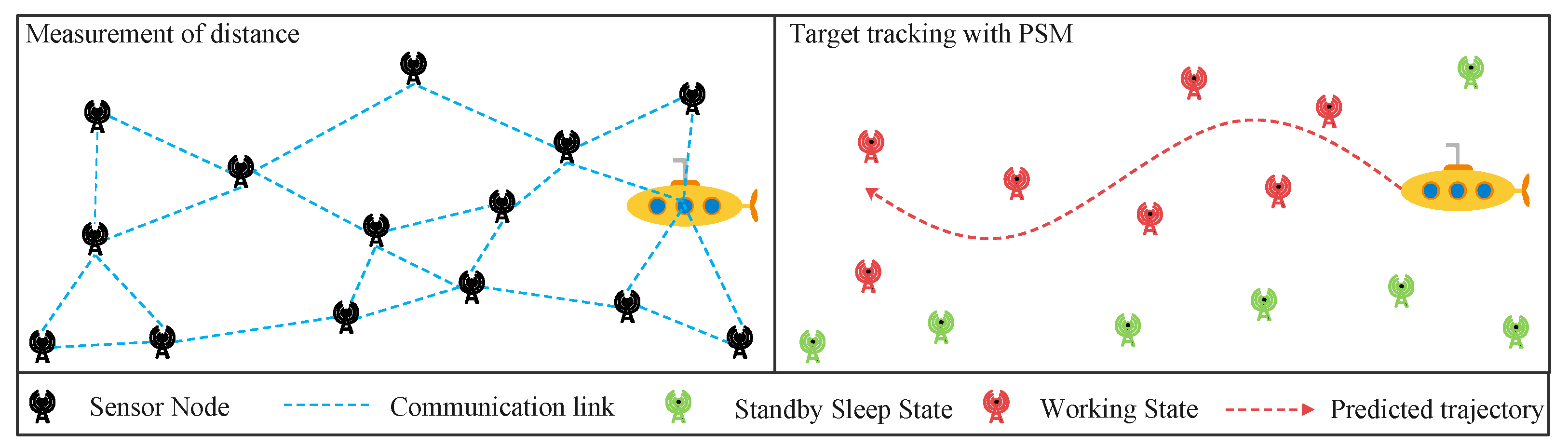
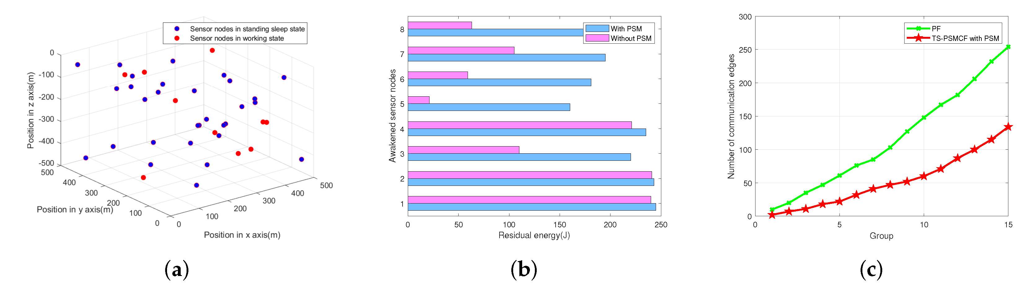
In this part of the experiment on energy consumption, two experimental scenarios are set. First, PSM is not included in the tracking task of TS-PSMCF. In the second experimental scenario, PSM is added to assist TS-PSMCF to complete the tracking task, and the schematic diagram of node operation is given in Figure 14a. Accordingly, Figure 14b is a comparison of the residual energy of the two scenarios. The vertical axis is the number of awakened nodes in the working state, and the horizontal axis is the residual energy. The maximum energy difference reaches 150 J, which will seriously affect the network life. For each group of columnar bars with fixed vertical axis value, the scheme of adding PSM has more residual energy. Therefore, TS-PSMCF assisted by PSM has more energy-saving performance. In the localization process, some localization units will be formed, which have multiple communication links (shown in the left half of Figure 9). The more links, the higher the energy consumption. Therefore, the statistical comparison of the number of communication links can also indirectly reflect the energy-saving performance of the tracking algorithm. The particle filter algorithm is selected as the comparison, because it estimates the target through particle swarm approximation, which belongs to the same type as the localization unit combination localization method, so it is the best choice for the comparison group. Comparison of the number of communication links in Figure 14c, whether PF or TS-PSMCF, shows that the number of communication links will increase with the increase of unit groups. However, the growth rate of PF is faster and its curve is steeper. Fortunately, the curve of TS-PSMCF is relatively flat. It has better control over the number of links and will not make the number of links grow out of control. Therefore, the TS-PSMCF has the highest energy saving level.

6. Conclusions

This paper studies the problem of target detection, localization, and tracking in underwater sensor networks. In order to eliminate the problems of excessive computation and high sampling frequency of traditional algorithms in target detection, an improved convolutional neural network is built in this paper. Then, considering the problem of clock asynchrony in practical application environment, this paper proposes a localization algorithm which can resist clock asynchrony. After localization, the system also needs to track the target. A tracking scheme based on weighted consensus algorithm and fusion filtering is proposed, which can track the target continuously. Moreover, this paper proposes a predictive switching mechanism to assist the operation of TS-PSMCF. The energy-saving effect of sensor nodes is realized, so as to prolong the network life. The clock model in this paper only involves two dynamic parameters, and the real clock problem is more complex. If the clock problem can be extended and the corresponding tracking algorithm can be designed, the monitoring and tracking level of underwater sensor networks will be greatly improved.

References

1. Khasawneh, A.M.; Altalhi, M.; Kumar, A.; Aggarwal, G.; Kaiwartya, O.; Khalifeh, A.; Al-Khasawneh, M.A.; Alarood, A.A. An Efficient Void Aware Framework for Enabling Internet of Underwater Things. J. Mar. Sci. Eng. 2021, 9, 1219. [Google Scholar] [CrossRef]
2. Ghoreyshi, S.M.; Shahrabi, A.; Boutaleb, T. A Novel Cooperative Opportunistic Routing Scheme for Underwater Sensor Networks. Sensors 2016, 16, 297. [Google Scholar] [CrossRef] [PubMed]
3. Ghoreyshi, S.M.; Shahrabi, A.; Boutaleb, T. An Opportunistic Void Avoidance Routing Protocol for Underwater Sensor Networks. In Proceedings of the 30th IEEE International Conference on Advanced Information Networking and Applications (IEEE AINA), Crans-Montana, Switzerland, 23–25 March 2016; pp. 316–323. [Google Scholar] [CrossRef] [Green Version]
4. Ghoreyshi, S.M.; Shahrabi, A.; Boutaleb, T.; Khalily, M. Mobile Data Gathering With Hop-Constrained Clustering in Underwater Sensor Networks. IEEE Access 2019, 7, 21118–21132. [Google Scholar] [CrossRef]
5. Ghoreyshi, S.M.; Shahrabi, A.; Boutaleb, T. A Stateless Opportunistic Routing Protocol for Underwater Sensor Networks. Wirel. Commun. Mob. Comput. 2018, 2018, 8. [Google Scholar] [CrossRef]
6. Alfouzan, F.A. Energy-Efficient Collision Avoidance MAC Protocols for Underwater Sensor Networks: Survey and Challenges. J. Mar. Sci. Eng. 2021, 9, 741. [Google Scholar] [CrossRef]
7. Songzuo, L.; Iqbal, B.; Khan, I.U.; Ahmed, N.; Qiao, G.; Zhou, F. Full Duplex Physical and MAC Layer-Based Underwater Wireless Communication Systems and Protocols: Opportunities, Challenges, and Future Directions. J. Mar. Sci. Eng. 2021, 9, 29. [Google Scholar] [CrossRef]
8. Liang, G.L.; Shi, Z.B.; Qiu, L.H.; Sun, S.B.; Lan, T. Sparse Bayesian Learning Based Direction-of-Arrival Estimation under Spatially Colored Noise Using Acoustic Hydrophone Arrays. J. Mar. Sci. Eng. 2021, 9, 22. [Google Scholar] [CrossRef]
9. Yamamoto, B.; Wong, A.; Agcanas, P.J.; Jones, K.; Gaspar, D.; Andrade, R.; Trimble, A.Z. Received Signal Strength Indication (RSSI) of 2.4 GHz and 5 GHz Wireless Local Area Network Systems Projected over Land and Sea for Near-Shore Maritime Robot Operations. J. Mar. Sci. Eng. 2019, 7, 16. [Google Scholar] [CrossRef] [Green Version]
10. Li, Y.Y.; Qi, G.Q.; Sheng, A.D. Performance Metric on the Best Achievable Accuracy for Hybrid TOA/AOA Target Localization. IEEE Commun. Lett. 2018, 22, 1474–1477. [Google Scholar] [CrossRef]
11. Gong, Z.J.; Li, C.; Jiang, F.; Zheng, J. AUV-Aided Localization of Underwater Acoustic Devices Based on Doppler Shift Measurements. IEEE Trans. Wirel. Commun. 2020, 19, 2226–2239. [Google Scholar] [CrossRef]
12. Cure, C.; Isojunno, S.; Siemensma, M.L.; Wensveen, P.J.; Buisson, C.; Sivle, L.D.; Benti, B.; Roland, R.; Kvadsheim, P.H.; Lam, F.P.A.; et al. Severity Scoring of Behavioral Responses of Sperm Whales (Physeter macrocephalus) to Novel Continuous versus Conventional Pulsed Active Sonar. J. Mar. Sci. Eng. 2021, 9, 444. [Google Scholar] [CrossRef]
13. Zhao, K.X.; Liang, J.L.; Karlsson, J.; Li, J. Enhanced multistatic active sonar signal processing. J. Acoust. Soc. Am. 2013, 134, 300–311. [Google Scholar] [CrossRef] [PubMed]
14. Josso, N.; Ioana, C.; Mars, J.; Gervaise, C. Source motion detection, estimation, and compensation for underwater acoustics inversion by wideband ambiguity lag-Doppler filtering. J. Acoust. Soc. Am. 2010, 128, 3416–3425. [Google Scholar] [CrossRef] [PubMed]
15. Mei, L.; Zhang, Q.Y.; Sha, X.J.; Zhang, N.T. Digital computation of the weighted-type fractional Fourier transform. Sci. China-Inf. Sci. 2013, 56, 12. [Google Scholar] [CrossRef] [Green Version]
16. Mabrouk, S.M.; Saleh, R.; Wazwaz, A. Investigation of ion - acoustic wave dynamics in unmagnetized grain plasmas. Chin. J. Phys. 2020, 68, 1–8. [Google Scholar] [CrossRef]
17. Tanwar, D.V.; Wazwaz, A. Lie symmetries and dynamics of exact solutions of dissipative Zabolotskaya–Khokhlov equation in nonlinear acoustics. Eur. Phys. J. Plus 2020, 135, 520. [Google Scholar] [CrossRef]
18. Karaca, Y.; Baleanu, D.; Zhang, Y.D.; Gervasi, O.; Moonis, M. Multi-Chaos, Fractal and Multi-Fractional Artificial Intelligence of Different Complex Systems; Elsevier: Amsterdam, The Netherlands, 2022. [Google Scholar]
19. Karaca, Y.; Baleanu, D.; Moonis, M.; Muhammad, K.; Zhang, Y.D.; Gervasi, O. Editorial Special Issue Section on Fractal Ai-Based Analyses and Applications to Complex Systems: Part I. Fractals 2021, 29, 2102002. [Google Scholar] [CrossRef]
20. Lou, G.; Shi, H. Face image recognition based on convolutional neural network. China Commun. 2020, 17, 117–124. [Google Scholar] [CrossRef]
21. Zhao, J.; Yang, S.; Li, Q.; Liu, Y.; Gu, X.; Liu, W. A new bearing fault diagnosis method based on signal-to-image mapping and convolutional neural network. Measurement 2021, 176, 109088. [Google Scholar] [CrossRef]
22. Deng, L.; Chu, H.; Shi, P.; Wang, W.; Kong, X. Region-Based CNN Method with Deformable Modules for Visually Classifying Concrete Cracks. Appl. Sci. 2020, 10, 2528. [Google Scholar] [CrossRef] [Green Version]
23. Sabir, Z.; Raja, M.A.Z.; Umer, M.; Shoaib, M. Design of neuro-swarming-based heuristics to solve the third-order nonlinear multi-singular Emden–Fowler equation. Eur. Phys. J. Plus 2020, 135, 410. [Google Scholar] [CrossRef]
24. Ahmad, A.; Husain, S.; Azeem, M.; Elahi, K.; Siddiqui, M.K. Computation of Edge Resolvability of Benzenoid Tripod Structure. J. Math. 2021, 2021, 9336540. [Google Scholar] [CrossRef]
25. Sabir, Z.; Raja, M.A.; Guirao, J.L.G.; Saeed, T. Swarm Intelligence Procedures Using Meyer Wavelets as a Neural Network for the Novel Fractional Order Pantograph Singular System. Fractal Fract. 2021, 5, 277. [Google Scholar] [CrossRef]
26. Yan, J.; Zhao, H.; Luo, X.; Chen, C.; Guan, X. RSSI-Based Heading Control for Robust Long-Range Aerial Communication in UAV Networks. IEEE Int. Things J. 2019, 6, 1675–1689. [Google Scholar] [CrossRef]
27. Poostpasand, M.; Javidan, R. An adaptive target tracking method for 3D underwater wireless sensor networks. Wirel. Netw. 2018, 24, 2797–2810. [Google Scholar] [CrossRef]
28. Sun, Y.L.; Yuan, Y.Z.; Li, X.L.; Xu, Q.M.; Guan, X.P. An Adaptive Sampling Algorithm for Target Tracking in Underwater Wireless Sensor Networks. IEEE Access 2018, 6, 68324–68336. [Google Scholar] [CrossRef]
29. Luo, J.H.; Han, Y. A node depth adjustment method with computation-efficiency based on performance bound for range-only target tracking in UWSNs. Signal Process. 2019, 158, 79–90. [Google Scholar] [CrossRef]
30. Braca, P.; Willett, P.; LePage, K.; Marano, S.; Matta, V. Bayesian Tracking in Underwater Wireless Sensor Networks With Port-Starboard Ambiguity. IEEE Trans. Signal Process. 2014, 62, 1864–1878. [Google Scholar] [CrossRef]
31. Zhang, D.; Liu, M.Q.; Zhang, S.L.; Zhang, Q.F. Non-Myopic Energy Allocation for Target Tracking in Energy Harvesting UWSNs. IEEE Sens. J. 2019, 19, 3772–3783. [Google Scholar] [CrossRef]
32. Braca, P.; Goldhahn, R.; Ferri, G.; LePage, K.D. Distributed Information Fusion in Multistatic Sensor Networks for Underwater Surveillance. IEEE Sens. J. 2016, 16, 4003–4014. [Google Scholar] [CrossRef]
33. Zhao, C.; Chen, J.; He, J.; Cheng, P. Privacy-Preserving Consensus-Based Energy Management in Smart Grids. IEEE Trans. Signal Process. 2018, 66, 6162–6176. [Google Scholar] [CrossRef]
34. Liu, J.; Wang, Z.; Zuba, M.; Peng, Z.; Cui, J.; Zhou, S. DA-Sync: A Doppler-Assisted Time-Synchronization Scheme for Mobile Underwater Sensor Networks. IEEE Trans. Mob. Comput. 2014, 13, 582–595. [Google Scholar] [CrossRef]
35. Xu, T.; Tang, Z.; Leus, G.; Mitra, U. Multi-Rate Block Transmission Over Wideband Multi-Scale Multi-Lag Channels. IEEE Trans. Signal Process. 2013, 61, 964–979. [Google Scholar] [CrossRef] [Green Version]
36. Jiang, J.F.; Han, G.J.; Guo, H.; Shu, L.; Rodrigues, J. Geographic multipath routing based on geospatial division in duty-cycled underwater wireless sensor networks. J. Netw. Comput. Appl. 2016, 59, 4–13. [Google Scholar] [CrossRef]
37. Terejanu, G.; Singla, P.; Singh, T.; Scott, P.D. Adaptive Gaussian Sum Filter for Nonlinear Bayesian Estimation. IEEE Trans. Autom. Control 2011, 56, 2151–2156. [Google Scholar] [CrossRef]
38. Barman, P.P.; Liu, Q.; Al-Mamun, M.A.; Schneider, P.; Mozumder, M.M.H. Stock Assessment of Exploited Sardine Populations from Northeastern Bay of Bengal Water, Bangladesh Using the Length-Based Bayesian Biomass (LBB) Method. J. Mar. Sci. Eng. 2021, 9, 1137. [Google Scholar] [CrossRef]
39. Xue, K.; Wu, T.Y. Distributed Consensus of USVs under Heterogeneous UAV-USV Multi-Agent Systems Cooperative Control Scheme. J. Mar. Sci. Eng. 2021, 9, 20. [Google Scholar] [CrossRef]
40. Liu, W.; Zhang, L.L.; Wang, Y.X.; Cheng, X.H.; Xiao, W.B. A Vector Wavenumber Integration Model of Underwater Acoustic Propagation Based on the Matched Interface and Boundary Method. J. Mar. Sci. Eng. 2021, 9, 24. [Google Scholar] [CrossRef]
41. Yan, J.; Zhang, X.; Luo, X.; Wang, Y.; Chen, C.; Guan, X. Asynchronous Localization With Mobility Prediction for Underwater Acoustic Sensor Networks. IEEE Trans. Veh. Technol. 2018, 67, 2543–2556. [Google Scholar] [CrossRef]
42. Feng, H.L.; Cai, Z.W. Target tracking based on improved cubature particle filter in UWSNs. IET Radar Sonar Navig. 2019, 13, 638–645. [Google Scholar] [CrossRef]
43. Carroll, P.; Mahmood, K.; Zhou, S.L.; Zhou, H.; Xu, X.K.; Cui, J.H. On-Demand Asynchronous Localization for Underwater Sensor Networks. IEEE Trans. Signal Process. 2014, 62, 3337–3348. [Google Scholar] [CrossRef]
44. Zhang, Y.; Chen, H.; Xu, W.; Yang, T.C.; Huang, J. Spatiotemporal Tracking of Ocean Current Field With Distributed Acoustic Sensor Network. IEEE J. Ocean. Eng. 2017, 42, 681–696. [Google Scholar] [CrossRef]
Figure 1. Network structure.
Jmse 10 00283 g001
Figure 2. 2D detection model.
Jmse 10 00283 g002
Figure 3. ST-BPN.
Jmse 10 00283 g003
Figure 4. Simulation example of D-FrFT.
Jmse 10 00283 g004
Figure 5. Gray image of the top view angle of Figure 4.
Jmse 10 00283 g005
Figure 6. Structure of M-CNN.
Jmse 10 00283 g006
Figure 7. Training images. (a) Positive image. (b) Negative image. (c) Negative image.
Jmse 10 00283 g007
Figure 8. Interaction of location information.
Jmse 10 00283 g008
Figure 9. Location information structure.
Jmse 10 00283 g009
Figure 10. PSM.
Jmse 10 00283 g010
Figure 11. Simulation of LA-AIC (first scenario). (a) The distribution position of sensor nodes. (b) Real distance and measured distance. (c) Ranging error.
Jmse 10 00283 g011
Figure 12. Simulation of LA-AIC (second scenario). (a) Real distance and measured distance. (b) Ranging error. (c) Estimation of clock information.
Jmse 10 00283 g012
Figure 13. Simulation of TS-PSMCF with PSM (tracking error). (a) The motion trajectory of the target and the tracking trajectory of the three algorithms. (b) Tracking error.
Jmse 10 00283 g013
Figure 14. Simulation of TS-PSMCF with PSM (energy consumption). (a) Location and status of sensor nodes. (b) Residual energy of network. (c) The number of communication edges.
Jmse 10 00283 g014