Article

Numerical Prediction of Convective Heat Flux on the Flight Deck of Naval Vessel Subjected to a High-Speed Jet Flame from VTOL Aircraft

1
Department of Naval Architecture and Ocean Engineering, Inha University, 100, Inha-ro, Michuhol-gu, Incheon 22212, Korea
2
Extreme Technology Research Center for Ship and Offshore Platform, Inha University, 100, Inha-ro, Michuhol-gu, Incheon 22212, Korea
*
Author to whom correspondence should be addressed.
J. Mar. Sci. Eng. 2022, 10(2), 260; https://doi.org/10.3390/jmse10020260
Submission received: 24 December 2021 / Revised: 4 February 2022 / Accepted: 5 February 2022 / Published: 14 February 2022
(This article belongs to the Special Issue Computational Fluid Mechanics)

Abstract

:
This study examines the heat flux and convective heat transfer generated when a vertical take-off and landing (VTOL) aircraft takes off and lands on the flight deck of a naval vessel. A procedure for analyzing the convective heat transfer imposed on the deck by the high-temperature and high-velocity impingement of a VTOL jet is described. For the analysis, the jet velocity and the deck arrival temperature were calculated by applying computational fluid dynamics (CFD), assuming that the heat flow is an impingement jet. The relationships between the diameter of the jet, the speed of impingement, and the exhaust temperature of VTOL are introduced to assess the inlet condition. Heat flow was analyzed using CFD techniques, and Reynolds-averaged Navier–Stokes (RANS) and k-ε models were applied to model the turbulent motion. A procedure for evaluating the convection coefficient and convective heat flux from the calculated local velocity and temperature is presented. Simultaneously, a method for compensating the convection coefficient considering the singular velocity at the stagnation point is proposed. Furthermore, the accuracy was verified by comparing the convective heat flux and deck temperature predicted using CFD with the existing experimental studies. Finally, by applying finite element analysis (FEA) based on the thermal-structural interaction, the magnitude of thermal deformation due to conductive temperature and heat flux was presented as a design application of the flight deck.

1. Introduction

Flame jets from vertical take-off and landing (VTOL) aircraft harm the flight decks of naval vessels, generating excessive thermal deformation and thermal stress. The purpose of this study is to predict the magnitude of the convective heat transfer of jet flames that generate thermal stresses on the flight deck. For predicting the distribution of local convective heat transfer, it is necessary to analyze the thermal flow and convective heat flux simultaneously. The turbulent thermal fluid flow of the VTOL represents an impinging jet. For predicting convective heat transfer, several variables such as the velocity and temperature of the flow and the temperature-dependent material properties must be considered. The complexity of the jet impingement makes it challenging to predict the convective heat transfer to surfaces that receive these violent flows.
Various studies have been conducted on the heat transfer of jet impingement for the Reynolds number, the shape and array of the nozzle, and the standoff distance of the nozzle and impingement wall. Most of them use both experimental measurement and numerical analysis to predict convective heat transfer. Jambunathan et al. [1] reviewed experimental data on heat transfer rates for circular jets impinging on a flat surface. The effects of the Reynolds number, jet-to-surface distance, nozzle geometry, and jet orientation and shape have been most widely studied. Katti and Prabhu [2] experimentally investigated the effect of the nozzle-to-plate spacing and Reynolds number on the heat transfer distribution to normally impinging circular air-jet on a flat surface. VTOL heat flow can be expressed as a turbulent thermal flow of exhaust gas on the thermal deck. Crosser [3] and Naval Surface Warfare Center (NSWC) research [4] performed real-scale experimental results for a VTOL. Crosser [3] experimentally presented the convective heat transfer coefficient and temperature distribution of VTOL exhaust gas. NSWC [4] measured the heat effect of a land-based experiment of a VTOL for the flight deck. This experiment presented the history of maximum temperature on the thermal deck according to the operating conditions of the VTOL
Zuckerman and Lior [5] presented a series of different turbulence models used to examine their performance in simulating jet impingement cooling of a flat target under a round jet. Pattamatta et al. [6] focused on the theoretical treatment of the problem by numerical model or experiments with laboratory-controlled systems using axisymmetric jets impinging on flat plates. Barata [7] performed laser doppler anemometry (LDA) measurements and numerical simulations for impinging jets and studied the effect of flow on the impinging jets below a VTOL aircraft in the ground. Matsumoto et al. [8] examined the heat transfer and the flow pattern from an impinging jet. However, the Reynolds number and scale frame jet VTOL are distinct problems from those in the investigated studies. Furthermore, several studies use a Nusselt number or convection coefficient with interest in heat convection at the stagnation point. Gauntner et al. [9] suggest that the local radial velocity gradient parameter at the stagnation influences stagnation point heat transfer coefficients. Because the horizontal velocity (parallel to the impingement wall) is zero in the stagnation region, Martin and Boyd [10] considered the vertical velocity of the arrival stream. Although several studies on jet impingement have proposed convection coefficient equations for various Reynolds numbers and nozzle sizes, it is difficult to use the proposed convection coefficient equations because the Reynolds number and nozzle size of VTOL jets are very large compared to the studies investigated.
Considering relatively little has been published about the computational model where the thermal deck is heated by hot impingement, this study aims to examine the heat transfer characteristics of a VTOL jet impinging onto the deck of a naval vessel. The primary goal of the present study is to numerically predict the distribution of convective heat flux delivered to the flight deck by the nozzle flame. The literature to date agrees on the use of computational fluid dynamics (CFD) using Reynolds-averaged Navier-Stokes (RANS) equations in a turbulence model to study the effect of the heat transfer rate between the jet gas and the heated surface. CFD enables simulating convective heat flux and heat energy transfer on the impingement wall. This study analyzes the heat flow behavior using a three-dimensional (3D) finite volume method and a k-ε turbulence model based on the RANS equation. Transient heat conduction and thermal-structural analysis are then introduced.

2. Problem Description of VTOL with an Impinging Jet

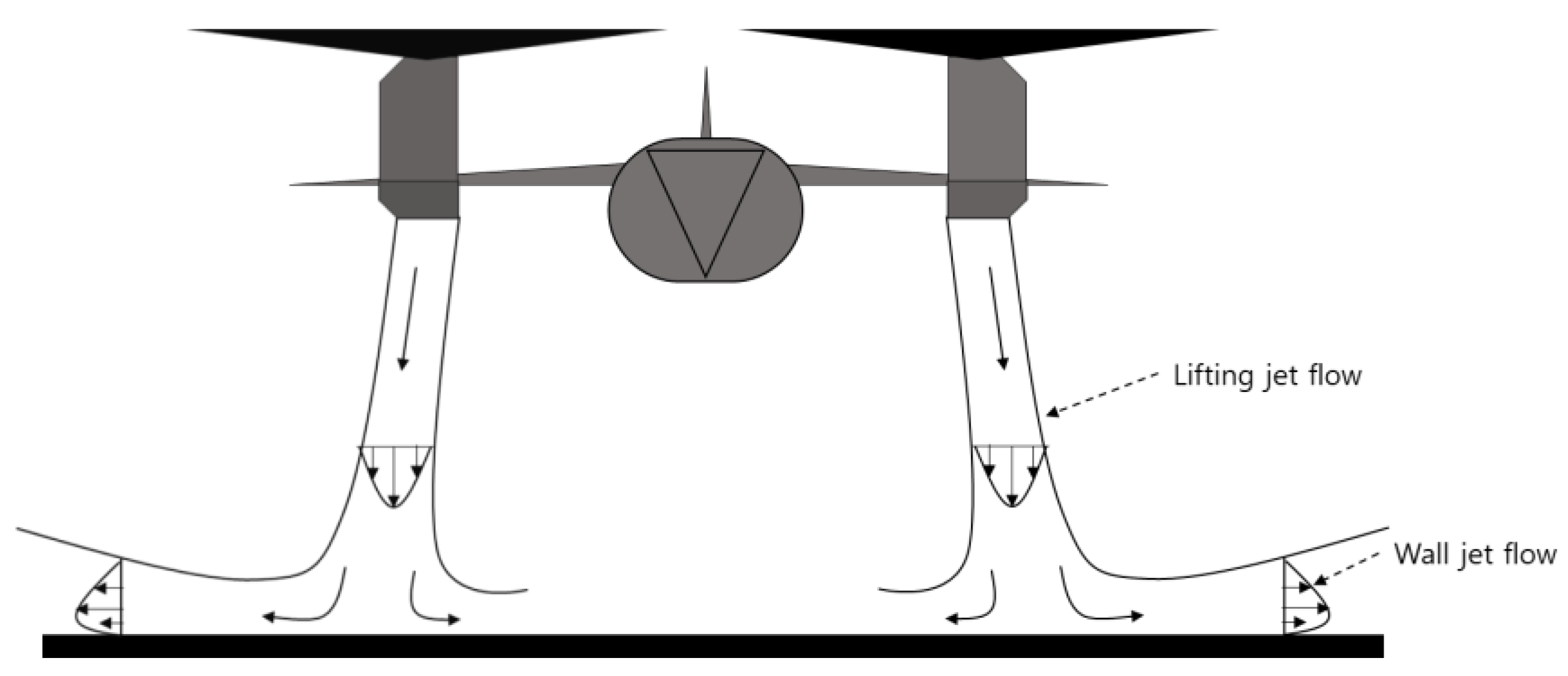
2.1. Characteristic of Heat Transfer by VTOL

VTOL aircrafts operate on small-to-medium aircraft carrier naval vessels. VTOL can hover, take off, and land vertically on the flight deck. This study is concerned with the exhaust flame of the MV-22 Osprey, a tilt-rotor type VTOL aircraft designed to operate on naval vessels. The Osprey is unique because it uses two engines positioned on fixed wingtips housed in nacelles that rotate to enable the MV-22 to land and take off vertically. For take-off and landing, it typically hovers using vertical nacelles and horizontal propeller. Exhaust heat from the turboprop engines can potentially damage the flight decks of a ship [11]. A schematic view of an impinging jet issuing from a nozzle of the VTOL on a flat deck is depicted in Figure 1, which was adapted from Annaswamy (2003) [12] and Choi (2005) [13]. The exhaust gas of VTOL is vertically sprayed from two turboprops to the flight deck during landing and take-off operation. A ground effect occurs because there are two adjacent jets, and each impinging downward jet creates an upward reingestion of exhaust gases.
Considering that the impingement of each jet onto a surface leads to a highly localized heat flow rate at the centroid, the modeling of one jet can lead to a more conservative prediction of the amount of heat flow. Therefore, the present study focuses on the flow of a single jet rather than the wake of the two jets. Two assumptions are made to adopt the one impingement in the analysis: (1) The distance between the two jets is far enough so that the thermal flow of the jet is not amplified. (2) The distance between the jet nozzle and the deck was assumed to be that of the landing status. Therefore, the distance between the jet flame and the deck when the VTOL landed, was reflected in the analysis. This is because the impinging flame transfers the largest heat to the deck at the moment of landing. The distance between the nozzle and the deck is fixed for the computational model. The gas flow rate, nozzle diameter and shape, standoff distance from the nozzle to the deck, and operation condition of VTOL should be considered in the CFD model. In all cases, the temperature and velocity distribution of the jet stream over the surface are required to approximate the magnitude of the heat flow. This heat flow has two consequences: (1) the high-temperature gradient generated by the heat flux and (2) the development of thermal stress and deformation of the flight deck.
Beltaos [14,15] and Rajaratnam [16] also divided the flow region into three regions (Figure 2): free jet, impingement, and wall jet. Figure 2 was modified from Beltaos [14,15] and Rajaratnam [16]. Katti and Prabhu [6] also divided the three regions of the impingement wall that extend to a distance from the center by the spread of the fluid; three regions can be listed, shown in Table 1 as suggested by Katti and Prabhu [2]. The hydrodynamic pattern of an impinging jet is crucial in studying the thermal effects of exhaust gas acting orthogonally on the target surface. The potential core can be observed until H/D = 4–6 (H: standoff distance from nozzle to deck, D: diameter of nozzle) and exists within the free jet region where the jet exit velocity is conserved and the turbulence intensity level is relatively low. A shear layer exists between the potential core and the ambient fluid where the turbulence is relatively high, and the mean velocity is lower than the jet exit velocity. The potential core diminishes in width as the shear layer around the jet grows. After the jet is fully developed, the axial velocity profile can be represented by a Gaussian distribution. The shear layer entrains ambient fluid and causes the jet to spread radially. Beyond the potential core, the shear layer spreads to the point where it penetrates the centerline of the jet. At this stage, the centerline velocity decreases, and the turbulence intensity increases. The stagnation region spans approximately 1.00 times the nozzle diameter for a laminar flow and varies in size for a turbulent flow [17,18,19,20]. The stagnation region includes the stagnation point where the mean velocity is zero. Within this region, the free jet is deflected into the wall jet flow and the flow is affected by the presence of the impingement surface.
The flow accelerates as it advances through the stagnation region due to the difference in static pressure between stagnation and an outer region. The flow velocity becomes higher than the velocity at the nozzle exit to maintain continuity of the flow. This region is called the acceleration region. The viscosity effects and loss of momentum cause the flow velocity to decrease gradually as the fluid progresses through the acceleration region parallel to the surface. The behavior of the wall jet region is characterized by a flow in the outward radial or spanwise direction. The wall jet region has a lower velocity than the acceleration region due to the loss of momentum. In this study, the characteristic of heat transfer developed in the stagnant region was analyzed in Section 4.4.

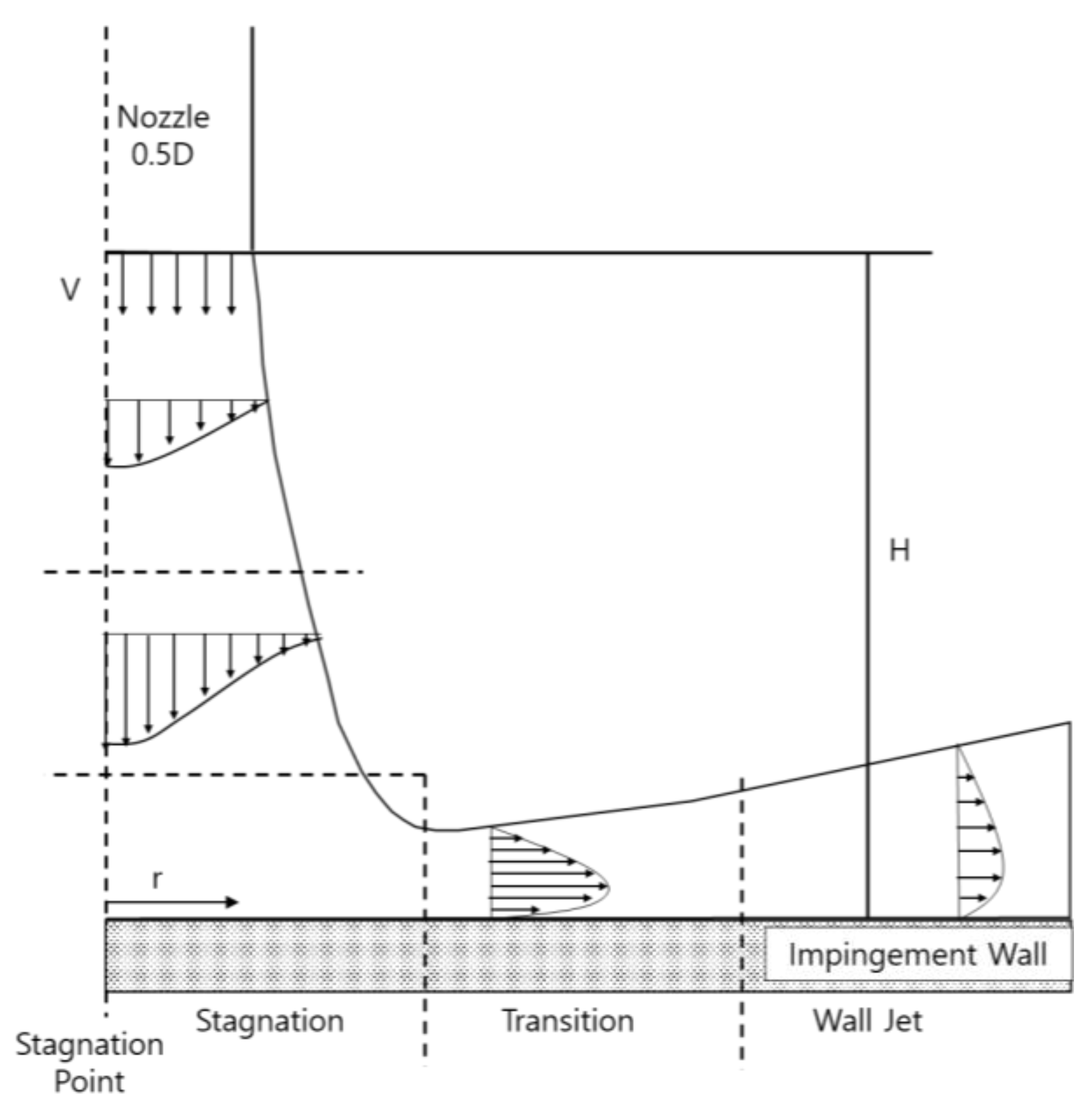
2.2. Schematic Formulation of Convective Heat Transfer by the Impinging Jet

Jet impingement heat transfer and flow features depend on parameters such as the jet’s Reynolds number, Prandtl number, nozzle geometry, spacing between nozzle exit and impingement plate, and distance from the stagnation point. The heat flow rate of impingement can be expressed as the convective heat transfer of a turbulent flow, where the convective heat transfer applies to heat transfer through a fluid to a solid. This mode propagates heat via the mixing of fluid regions on both molecular and large scales. The heat flux from the jet fluid to the target surface can be described by Newton’s law as:
q = h   ( T s T j e t ) ,
where q is the convective heat flux and h , T s , and T j e t are the convection coefficient, the temperature on the target surface exposed to the jet flow, and the temperature of a jet fluid, respectively. The convection coefficient is derived from the Nusselt number ( N u ), as defined by Equation (2).
h = N u k Characteristic   lengh = N u k D ,
where k represents the thermal conductivity. The Nusselt number ( N u ) on the impinging wall is represented by the functions of the jet Reynolds number ( R e ) , Prandtl number ( P r ), and H / D , where H is the stand-off distance from the jet nozzle to the wall, respectively [2,17,21]. Because D is constant in this study, the Nusselt number can be expressed by the function of both the Reynolds number and the Prandtl number. Therefore, the numerical result of the jet flow is used to find both the Reynolds number and the Prandtl number.
The next section presents the results of the Nusselt number predicted based on the resultant motion of the jet flow. For the Nusselt number, the Reynolds number ( R e ) is determined according to the nozzle diameter ( D ) and jet velocity ( V ) as ρ f V · D / μ f , where μ f is the viscosity of the jet fluid. In this study, R e is adjusted by a calibrated velocity at the stagnation point, as explained in Section 4.4 because ν is a temperature-dependent variable used in calculating the Reynolds number. The Prandtl number ( P r ) means the ratio of fluid thermal diffusivity to viscosity and is obtained by ν/α, where ν and α means the kinematic viscosity and thermal diffusivity of the jet fluid, respectively. Based on the definition of thermal diffusivity, the value of α can be calculated by k / ρ c , where ρ and c denote the density of exhaust gas and the specific heat, respectively. The value of the Prandtl number is approximately 0.7~0.8 in the gas state [22]. Therefore, the Nusselt number is expressed by a function of R e and P r in Equation (3).
N u = f ( R e ,   P r ,   with   constant   H / D ) .
Finite element analysis (FEA) modeling of heat conduction and thermal deformation inside the impinging wall can then be implemented based on the heat flux models, heating and cooling boundary conditions, and temperature-dependent material properties. Based on the above equations, this paper divides the heat transfer behavior of exhaust gas into three steps, as depicted in Figure 3.
First, the heat convection coefficient is calculated from the thermal flow behavior predicted by the analysis. The temperature distribution and velocity and pressure of the jet flow on the surface are then used to predict the Nusselt number and calculate the convection coefficient. Furthermore, the Reynolds number and Prandtl number are predicted. Second, the convective heat transfer coefficient is compensated by considering the vertical velocity and the dynamic pressure in the centroid stagnation zone. Third, the convective heat transfer coefficient predicted in the second step is applied to the coupled thermal-structural FEA. The coupled thermal-structural FEA is used to calculate the temperature distribution, thermal deformation, and thermal stress field inside the flight deck. The exhaust gas temperature distribution and dynamic pressure of impacting flow on the deck were applied as the load conditions.

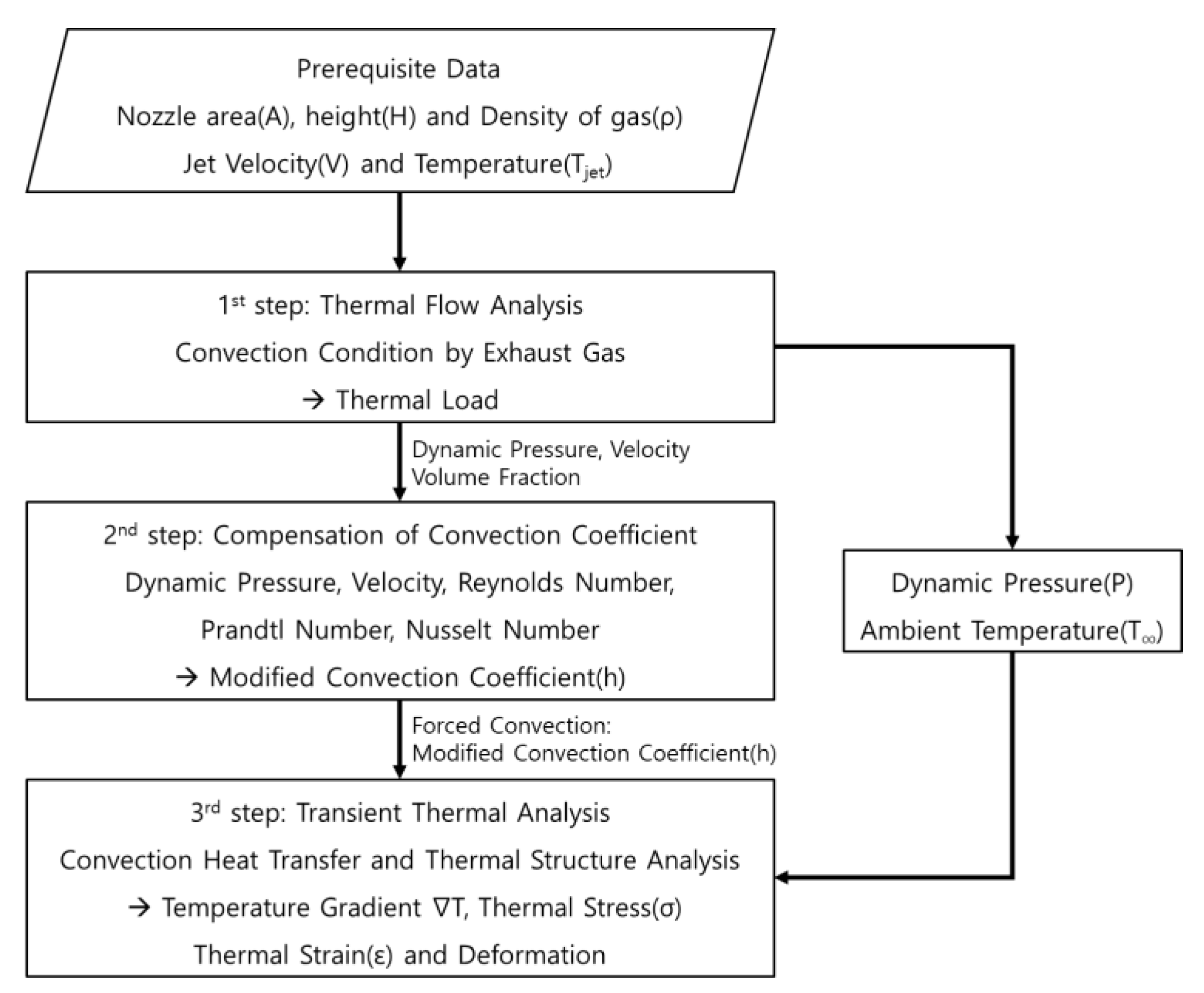
2.3. Governing Equation

Many studies [5,23,24] have shown that CFD can be used to solve the convective heat transfer of impinging jets. In this study, a numerical procedure that simulates the thermal flow of VTOL impingement was performed using ANSYS™ CFX Solver® under Workbench™ version 2021R1 (ANSYS Inc., Canonsburg, PA, USA). The equations describing the thermal flow of the impinging jet are represented by transport equations of momentum (Navier-Stokes equations) and energy (heat diffusion equation for the flow), developed from the mass conservation law (the continuity equation), momentum, and energy conservation (Olsson et al. [23]). The thermal flow is governed by the incompressible form of the RANS equations and by the equations describing the transport of energy, momentum, and energy [23].
  U j x j = 0 ,
ρ U i t + ρ ( U i U j ) x j = P x i + x j ( τ i j + τ i j t u r b ) ,
ρ c p T t + ρ c p ( U j T ) x j = x j ( q j + q j t u r b ) ,
where U i is the velocity of the fluid, ρ is the density of the fluid, τ ij is the Reynolds shear stress, c p is the specific heat, T is the temperature, and q i is the heat flux. P is the pressure, and superscript t u r b is the turbulence. Those variables are defined by: τ i j = μ ( U i x j + U j x i ) , τ i j t u r b = ρ u i ¯ u j ¯ , q j = μ c p P r T x j , q j t u r b = ρ c p u j ¯ T ¯ , where μ is the dynamic viscosity of fluid, u i and T are the fluctuating velocity and temperature, and P r is the Prandtl number. It would be impossible to solve these equations analytically because of non-linearity and the stochastic nature of turbulence. The additional terms that appear due to averaging the velocity and temperature are the Reynolds stresses and the turbulent heat flux. These models are the closure problem of turbulence.
Angioletti et al. [24,25] extensively investigated the flow field behavior in the vicinity of the stagnation region. They found that the k-w SST(Shear Stress Transport) model produces suitable results for a lower Re, while k-ε performed better for a high Re. Furthermore, in the study by Achari and Das [26] and in the studies by Coussirat [27,28], the standard k-ε model was adopted. The standard k-ε model is widely used and has relatively high accuracy for fluid flow analysis. With the standard two-equation k-ε model, the turbulent viscosity is evaluated from μ t = ρ C μ k 2 ε . where μ t is the turbulent viscosity, k is the turbulent kinetic energy, ε is the dissipation rate of the turbulent kinetic energy, C μ is a turbulence constant, and ρ is the density of the fluid. The turbulent kinetic energy, k , and the dissipation rate of turbulent kinetic energy, ε , are obtained by solving a conservation equation for each of these two quantities. Those equations are defined by Equations (7) and (8).
ρ k t + ( U j T ) x j = x j [ ( μ + μ t σ k ) k x i ] + P k ρ ε + P k b ,
ρ ε t + ( ρ U j ε ) x i = x i [ ( μ + μ t σ ε ) ε x i ] + ε k ( C ε 1 P C ε 2 ρ ε ) ,
where P k is the production rate of the turbulent kinetic energy defined as P k = ρ u i u j ¯ U j x j . C μ , σ ε , σ k , C ε 1 , and C ε 2 are empirical constants as shown in Table 2. These default values are defined from experiments with air or water for fundamental turbulent shear flows including homogeneous shear flows and decaying isotropic grid turbulence. [29,30,31].

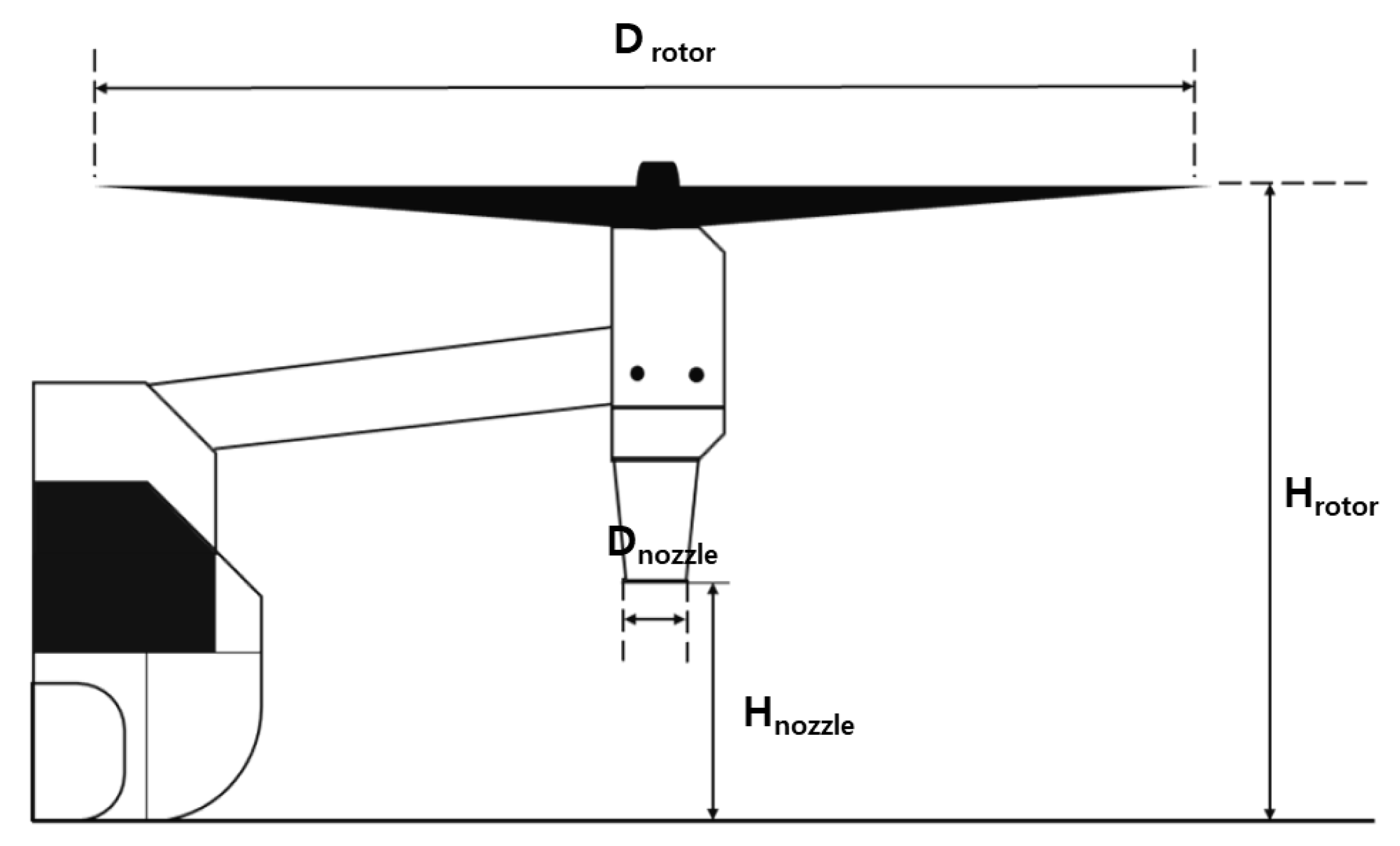
3. VTOL Simulation Model

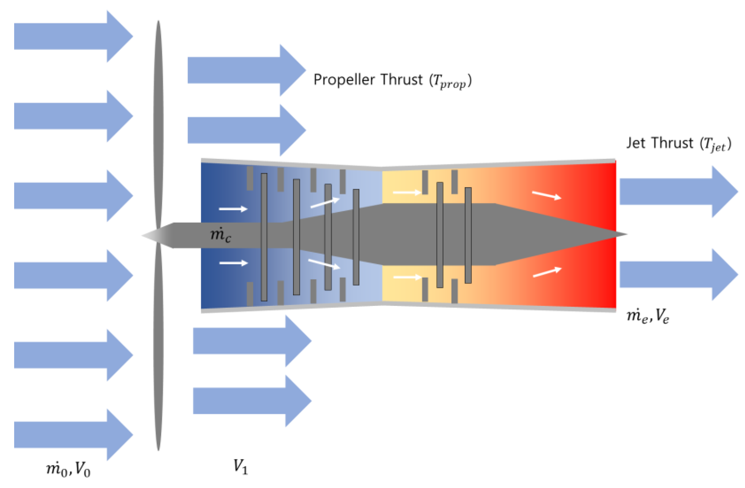
3.1. Estimation of Nozzle Velocity

In this study, it is assumed that the VTOL engine is a turboprop type, and the schematic view of that engine’s propulsion is illustrated in Figure 4. The turboprop simplifies the VTOL thrust power so that the exhaust velocity can be estimated based on the two types of thrust with the propeller ( T p r o p ) and turbojet ( T j e t ) .
Bolkcom [32] suggests that the maximum weight of the take-off ( W ) was about 25 tons (55,000 lbs). The sum of thrust must be equal or greater than the weight of the VTOL to hover or take off. Benson [33] expressed the thrust force of turboprop as in Equation (9). Rotaru and Todorov [34] expressed the propeller thrust as (10) for the VTOL to maintain the hovering state.
W =   Trust = 2 T p r o p + 2 T j e t = 2 ( m 0 ˙ ( V 0 V 1 ) + m e ˙ ( V e V 1 ) ) = 244.8 [ k N ] ,
T p r o p = m 0 ˙ ( V 0 V 1 ) = 2 ρ a A p V 1 2 ,
T j e t = m e ˙ ( V e V 1 ) = ρ e A e V e ( V e V 1 ) ,
where T p o r p is the thrust of a propeller, ρ a is the density of air, A p is the area of a propeller, V 1 is the induced velocity, T j e t is the thrust of a jet, ρ e is the density of exhaust gas, A e is the area of a nozzle, and V e is the exhaust gas velocity. The predicted VTOL velocity is 21.2 m/s [35]. Assuming that the motion of the VTOL is hovering, and the turboprop thrust force is the same as the weight of the VOTL, the exhaust gas velocity is assumed to be approximately 105 m/s.

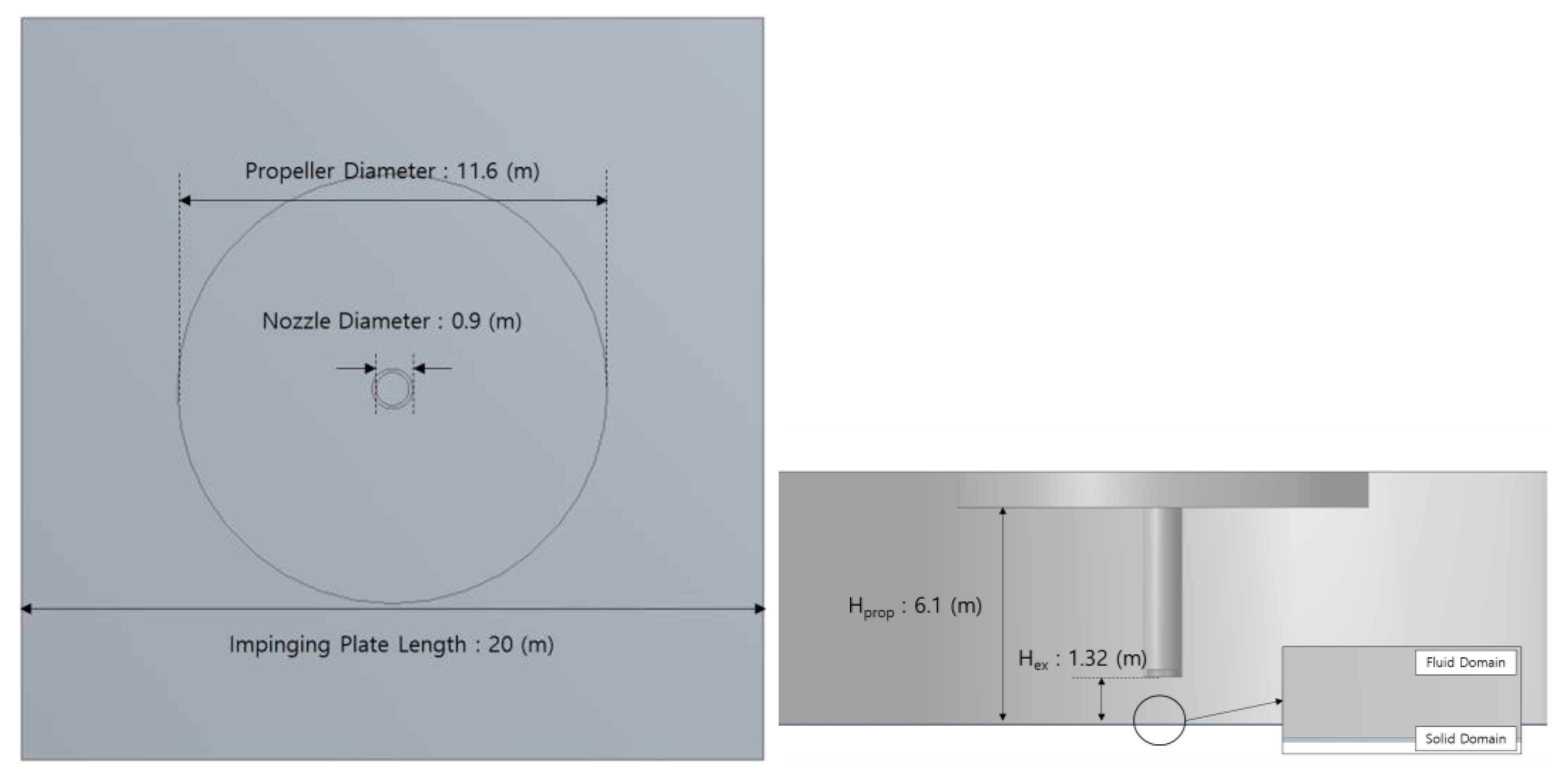
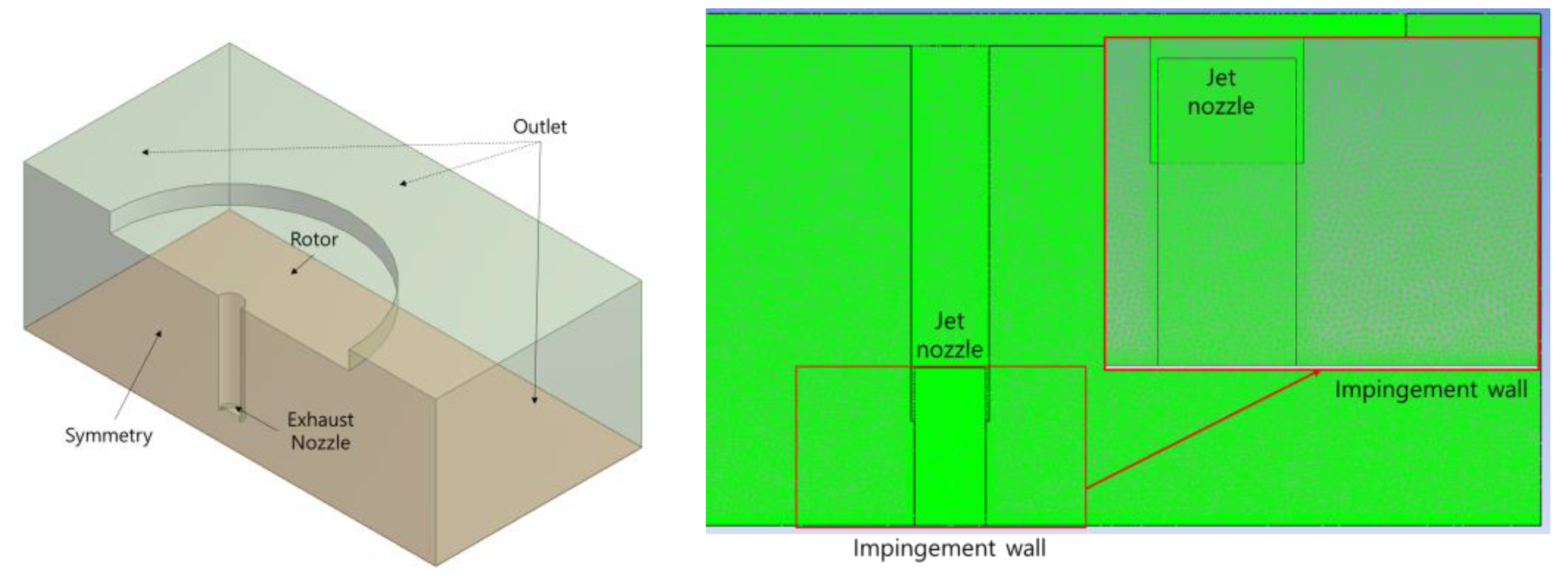
3.2. Description of Simulation Model Set Up

The steady-state analysis in three dimensions of the heat transfer associated with the local Nusselt numbers from an exhaust jet impinging on a solid were performed in CFX. The Nusselt number describes the dimensionless heat transfer represented by convective heat flux, while the Reynolds number is based on the jet velocity and the width of the jet. This study was assumed to be completely turbulent when exiting the nozzle and adiabatic at the solid wall. The simulation model was defined by simplifying the geometry and the domain (Figure 5).
The length of an impingement wall (L) is defined as r/D = 11(L = 10,000 mm) from the center. The jet nozzle and propeller diameters are 900 mm and 11,580 mm, and their heights from the impingement wall are 1320 mm and 6100 mm. The geometry specifications of the analysis model are summarized in Table 3, and the simulation model is depicted in Figure 6.
The parameters for the computational domain and the boundary conditions for the simulations are summarized in Table 4 and Figure 7. CFD methods based on unstructured grids have the advantage of efficiently handling complex geometries and can improve solution accuracy by refining cells locally as required. In this study, unstructured volume meshes were created using ANSYS 2021 R1 Meshing tool (ANSYS Inc., Canonsburg, PA, USA). Although an unstructured mesh consisting of tetrahedral elements was generated, the finer mesh was generated in the nozzle and impinging wall to compute the local velocity and temperature in the region.
For analysis efficiency, a half-model with a symmetrical condition applied at the center was used. The k-ε model was adopted for the turbulence model, and the analysis domain is defined as air and exhaust gas. The inlet condition of the propeller is air at 21.2 m/s and 25 °C; the inlet condition of a jet nozzle is exhaust gas at 100 m/s and 260 °C. An outlet with opening condition (Zero relative pressure) was given to the side walls of domain where the exhaust gas exits. The inlet and outlet boundary conditions used in the analysis are described in Figure 7. The values of the initial conditions and boundary conditions are also described in Table 4.
In order to check the grid dependence on the convergency of temperature and velocity, the results at the stagnation region according to the grid sizes are summarized in Table 5. Our values of interest are the velocity and temperature of flow, we make sure that these have converged to a steady value when the grid size is less than 80 mm. Ensuring that these values have reached an almost steady solution, the grid density of 21,791,040 elements for 50 mm was chosen for the CFD simulation.

4. Numerical Results and Discussion

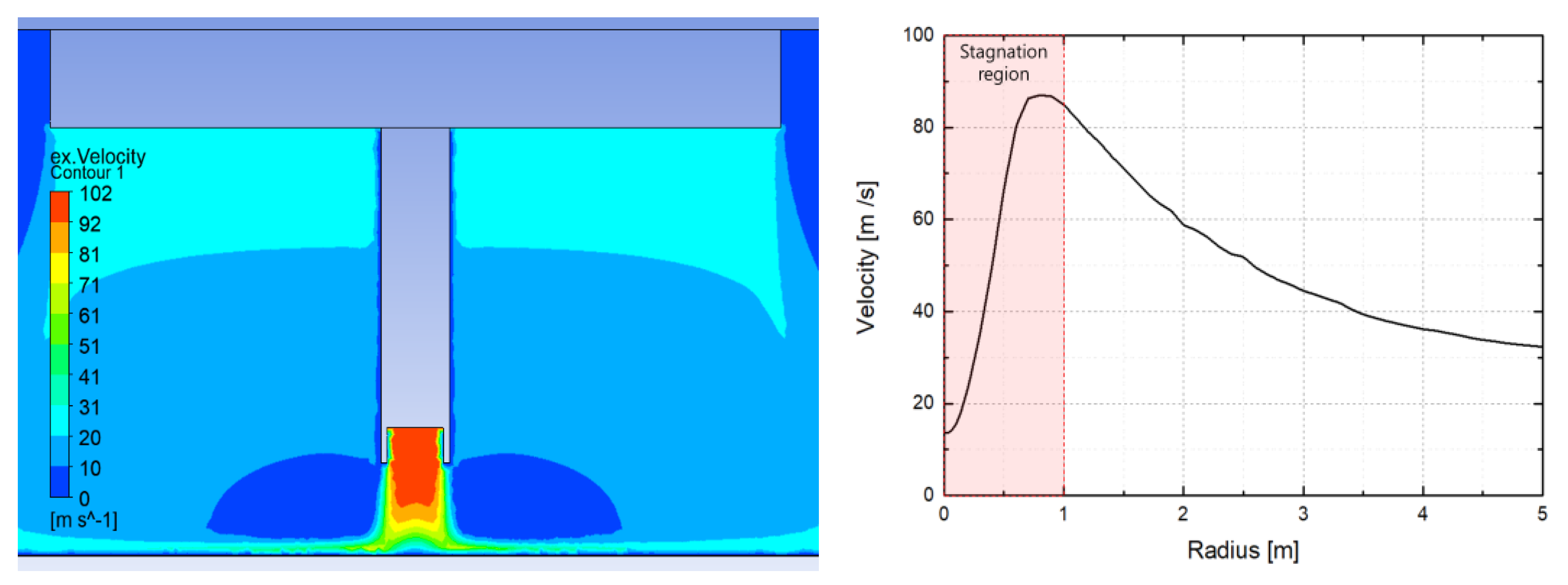
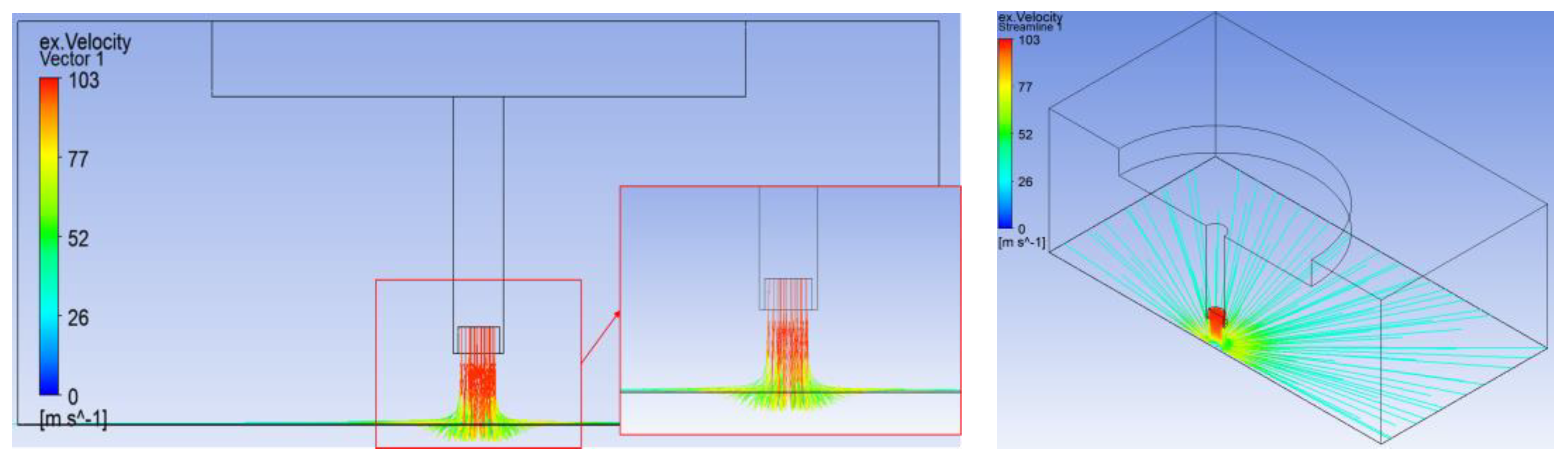
4.1. Velocity and Streamline of the Exhaust Gas

The fully developed turbulent 3D, steady, incompressible, single confined impinging jet flow is numerically simulated. The radial-velocity profiles of exhaust gas in the impingement wall are also depicted in Figure 8, revealing that the velocity in the stagnation region is much lower than in the other locations. Furthermore, the velocity vector and streamline distributions are depicted in Figure 9. The stagnation region is characterized by the dramatic curvature caused by the flow obstructing the impingement wall. The local radial velocity gradient is a parameter influencing the heat transfer coefficients.

4.2. Volume Fraction of the Exhaust Gas

Volume fraction represents the ratio of exhaust gas to air. CFX calculates the convection coefficient based on momentum without considering the volume fraction of exhaust [36]. That is, despite the low volume fraction of exhaust gas, CFX yields an excessive convective heat transfer coefficient. As shown in Figure 10, a large convective heat transfer coefficient is calculated despite the very low volume fraction of the exhaust gas on the upper surface. Therefore, it is necessary to correct the convection coefficient by multiplying the volume fraction of the injection gas. The distribution of the volume fraction of exhaust gases at the impact wall is shown in Figure 11.

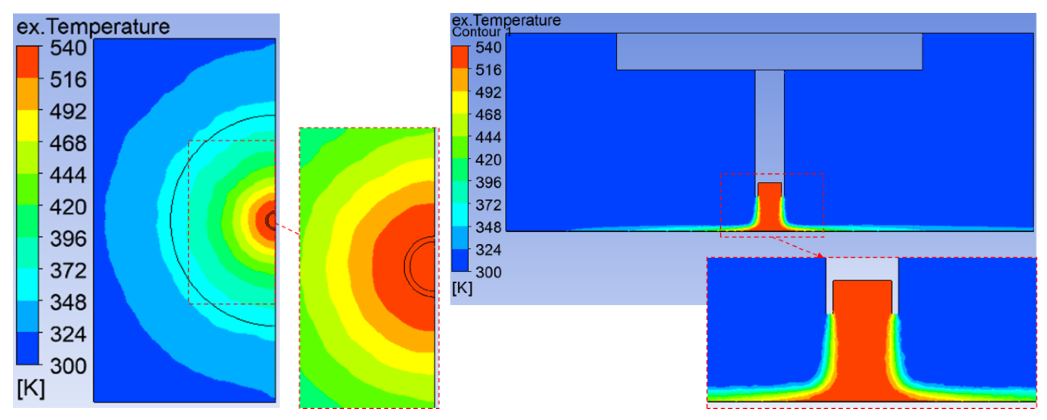
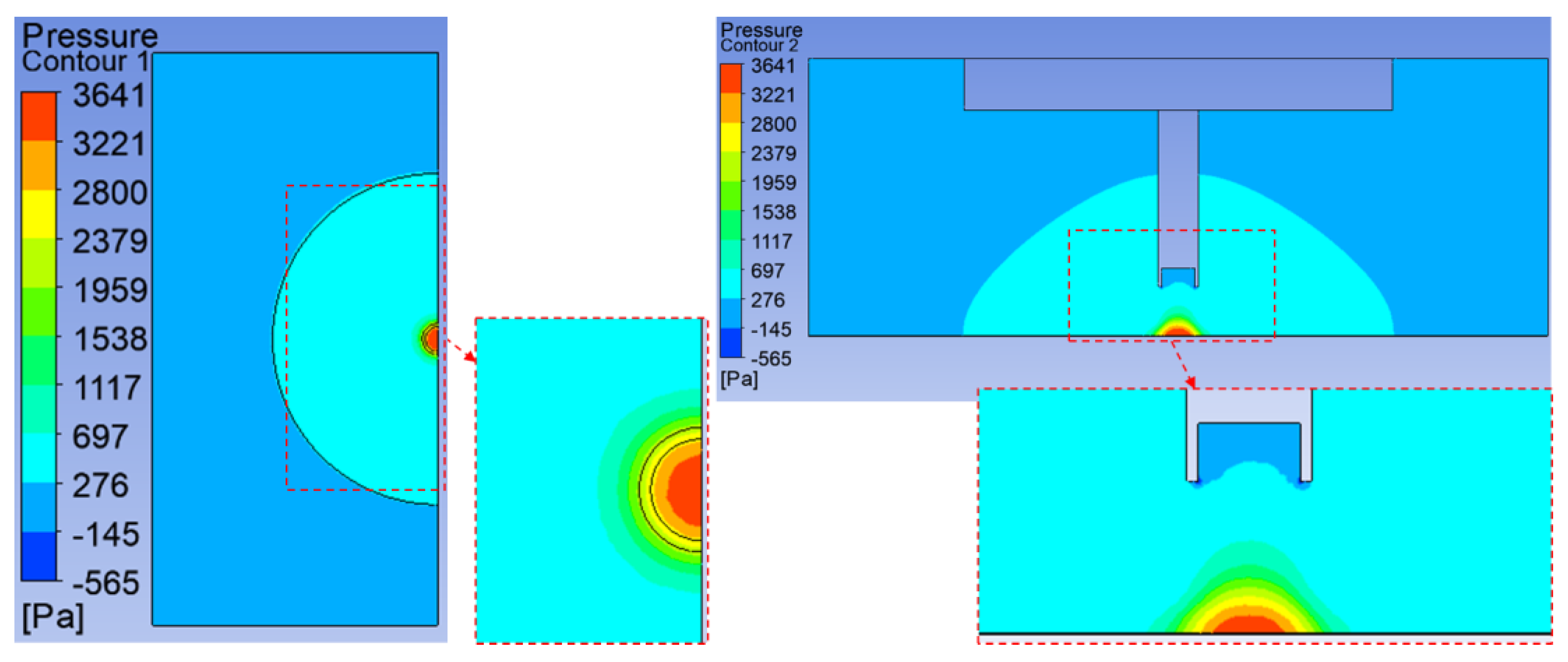
4.3. Temperature and Pressure Distribution of Exhaust Gas

This section analyzes the temperature and dynamic pressure distribution as factors considered for thermal-structural analysis of the deck and temperature. The dynamic pressure distribution as r/D is depicted in Figure 12. The temperature distribution and the contour of the impingement gas are depicted in Figure 13. The maximum temperature reaches 545 K (276.6 °C), and the average temperature is 542.7 K (271.8 °C) in the stagnation region. As the radial distance increases, the temperature decreases on the wall jet region. Not only the temperature and the convection coefficient but also the dynamic pressure of exhaust gas is acting on the deck. The maximum pressure of exhaust gas is 3.8 kPa; the pressure profile is depicted in Figure 14.

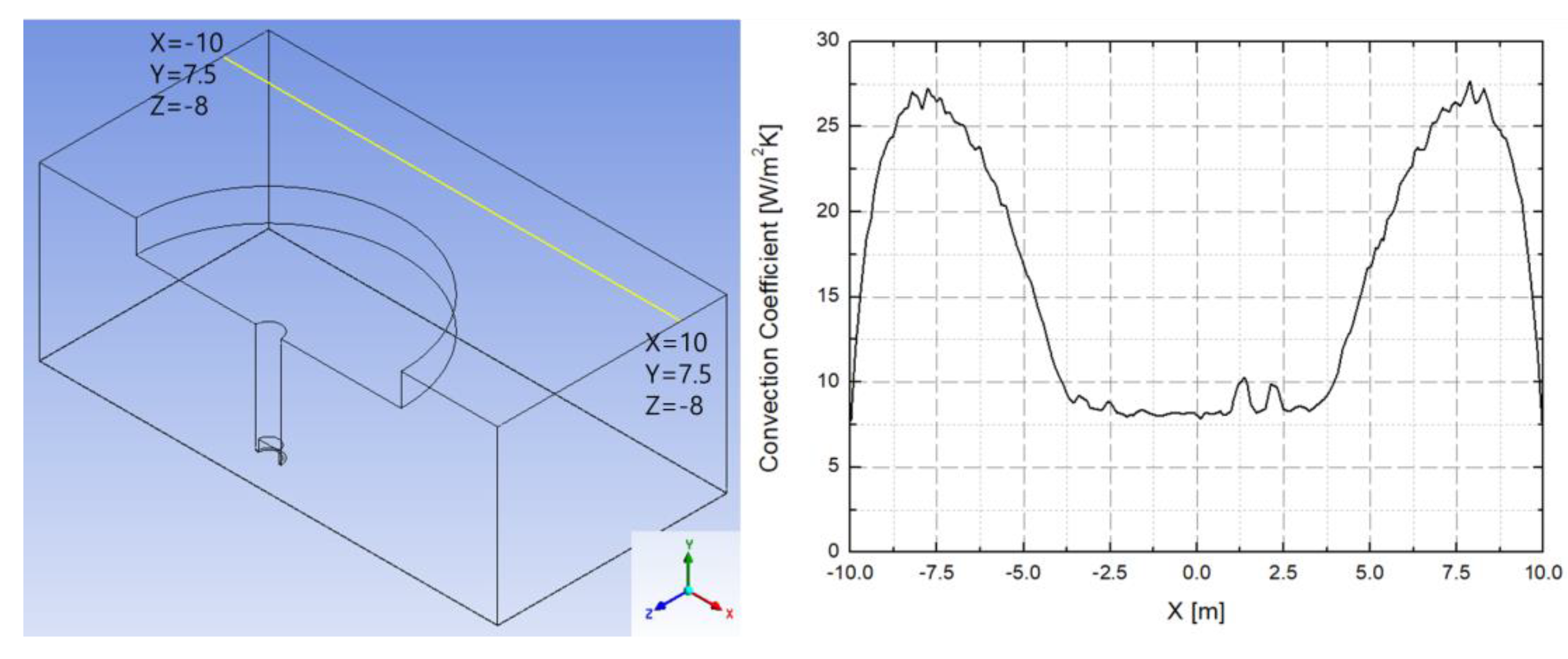
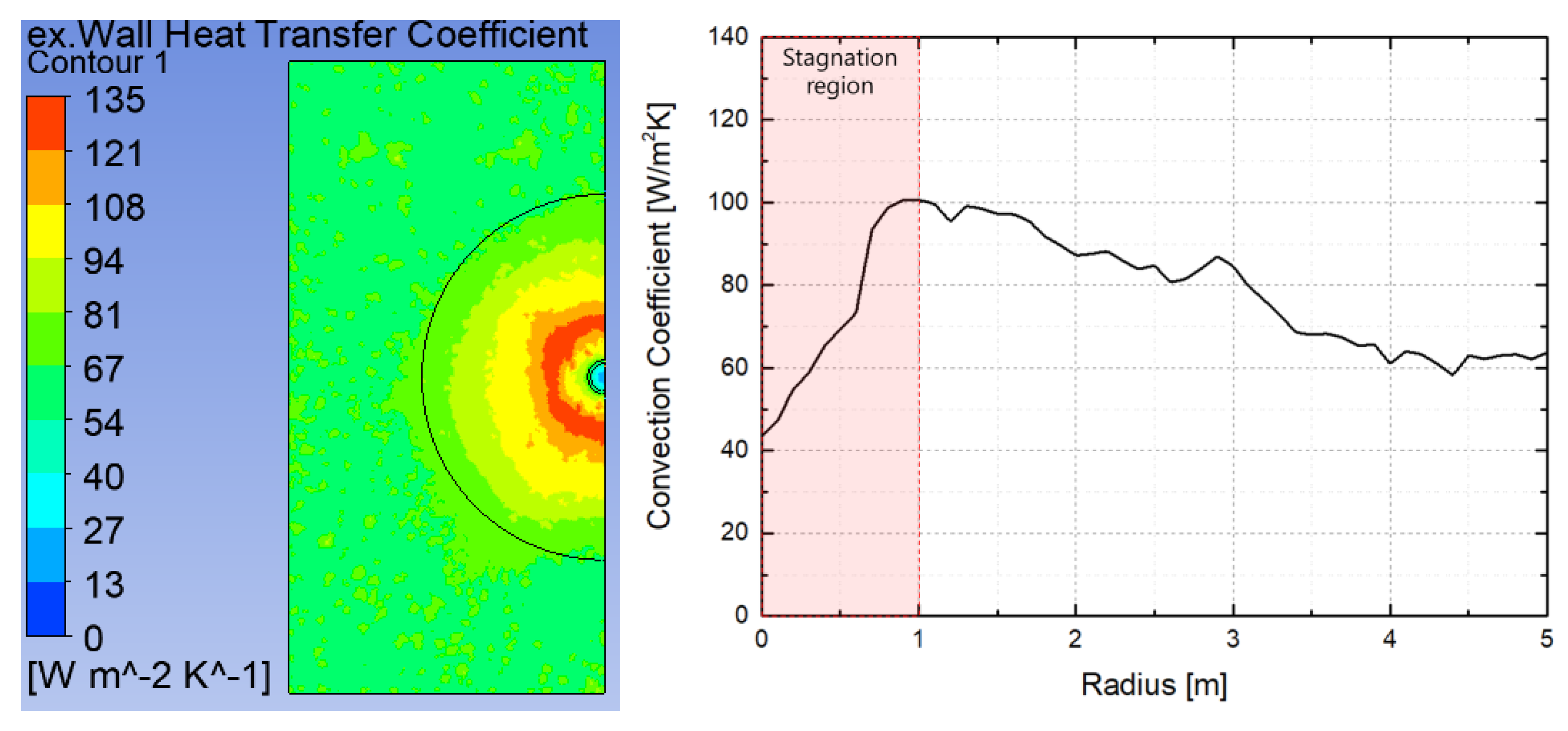
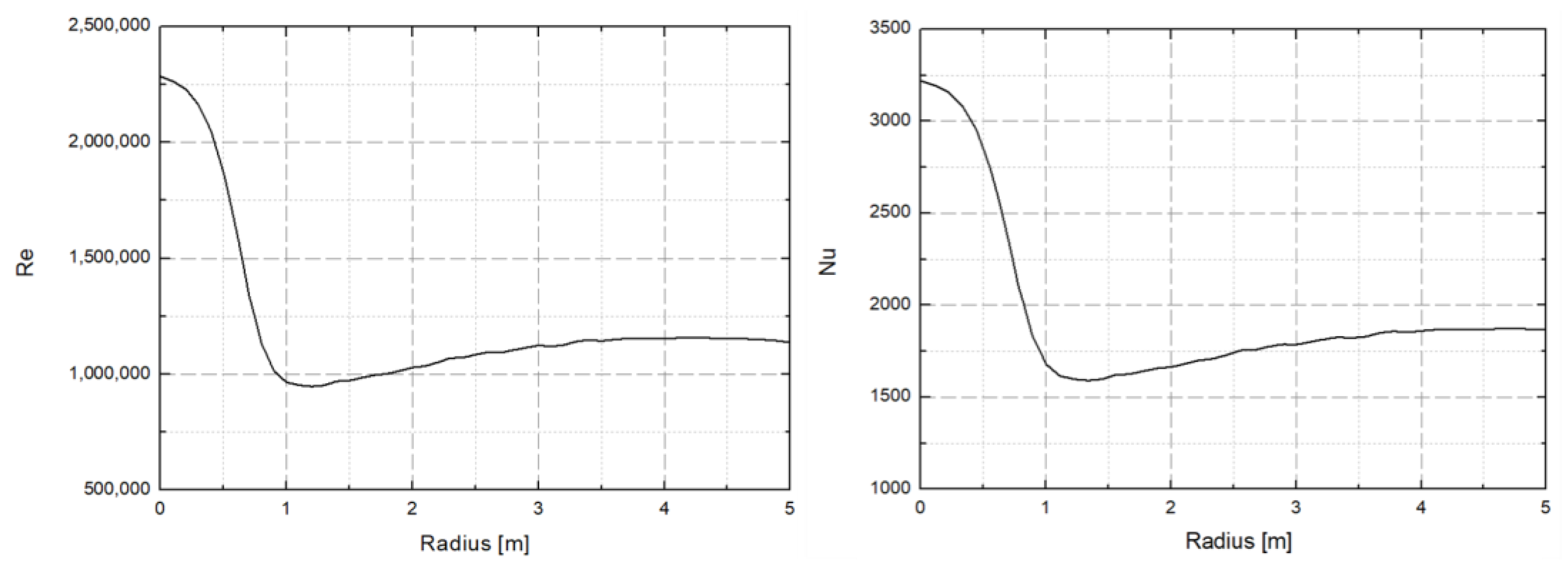
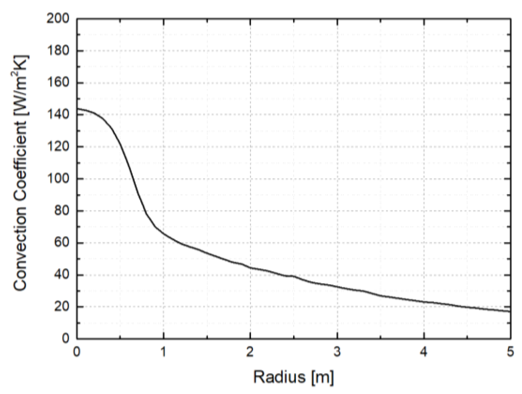
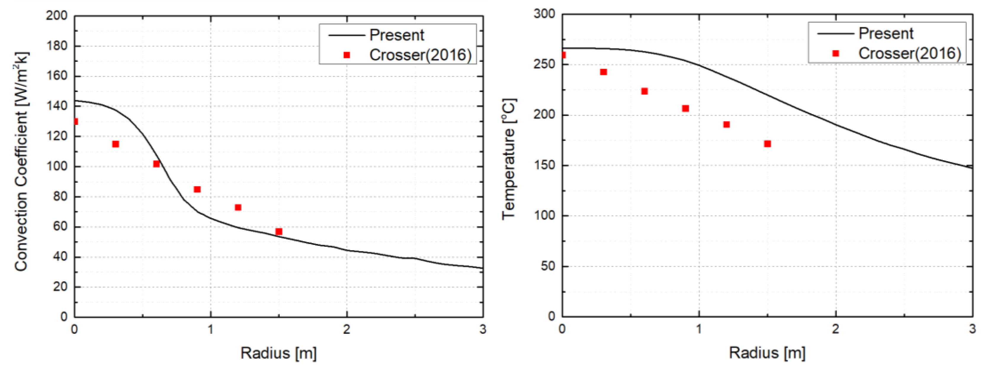
4.4. Calibration of Convection Coefficient at the Stagnation Point

The convection coefficient is the major parameter of thermal load to evaluate the thermal effect on the deck. Although similar experiments [3,4] showed that the convection coefficient at the stagnant point was higher than that in the transition region, the convective coefficient predicted by CFX yields a maximum value in the transition region and a lower value in the stagnant region as shown in Figure 15. This discrepancy comes from the calculation procedure of CFX to compute the convection coefficient. CFX uses the difference between the temperature of the exhaust gas and the temperature of the impinging wall in steady state to calculate the convection coefficient as it calculates the convection coefficient through the equation h = h e a t   f l u x / ( T s T ), where T s and T represent the temperature of the impinging wall and the gas, respectively [36]. The higher the temperature of the impinging walls, the lower the convection coefficient, whereas the opposite is observed in the experiment. Hannat and Morency [37], Park et al. [38], and Heyrichs et al. [39] also observed the heat flux profile falling at the stagnation point in the CFD analysis of the jet. The unreasonable profile of heat flux at the stagnation point is also due to the zero velocity at the stagnation point above the heat conduction media. Several numerical studies suggested methods to correct the convection coefficient and the Nusselt number at the stagnation point. In particular, they suggested that it is reasonable to consider the vertical velocity just before the jet impacts the impinging wall in order to calculate a reasonable convection coefficient at the stagnation point. Katti and Prabhu [2] and Vlachopoulos and Tomich [22] successfully presented an interpolation method for the Nusselt number at stagnation using the velocity field of fluid above the impinging wall. Therefore, it is reasonable to obtain the convection coefficient directly from the flow velocity and temperature at the moment of reaching the wall. That is, the Prandtl number, Reynolds number, Nusselt number, and convection coefficient should be assessed from the flow field of exhaust gas just above the wall. Therefore, in this study, the convection coefficient at the stagnation point was assessed based on the temperature and velocity above the impinging wall.
According to Gauntner et al. [9], the local radial velocity gradient at stagnation affects the stagnation point heat transfer coefficient. The local radial velocity gradient at the stagnation point is also considered as the static pressure distribution at the stagnation point, assuming incompressible flow. Therefore, in this study, the local convective heat transfer coefficient of the stagnation point was corrected by reflecting the flow pressure and velocity immediately before the impinging at the stagnation point, as defined by Equation (12).
V e q ( r ) = 2 ( P ( r ) ρ ( r ) + V 2 ( r ) 2 ) ,
where V e q ( r ) , P 1 ( r ) , and ρ ( r ) are the equivalent velocity, pressure, and density of the exhaust gas at local point r, respectively. Furthermore, the Reynolds number in Equation (3) was calculated using the equivalent velocity with the dynamic viscosity and the diameter of a nozzle as Equation (13) in the impingement jet problem [1,2,5,6,22]. The maximum value is approximately 2.2 million at the stagnation point. The Prandtl number is the ratio of dynamic viscosity and thermal diffusion, as defined by Equation (14). In this study, Pr(r) is obtained at the local point r and its range is calculated as 0.7–0.71.
The local Nusselt number ( N u ( r ) ) can be estimated with the local Prandtl ( P r ( r ) ) and local Reynolds ( R e ( r ) ) numbers defined by Equation (15) [40]. The distribution of the local Nusselt and Reynolds numbers is depicted in Figure 16. The convection coefficient was then calculated from the equivalent velocity, and an appropriate thermal load distribution was presented.
R e ( r ) = ρ f ( r )   V e q ( r ) · D n o z z l e μ f ( r ) ,
P r ( r ) = c f ( r ) · μ f ( r ) k f ( r ) ,
N u ( r ) = 0.0308   R e ( r ) 0.8   P r ( r ) 1 3 .
The heat flux by convection of exhaust gas analysis neglects the effect of a volume fraction of exhaust gas in the heat transfer. The efficiency of heat transfer where the VF is 1 and close to 0 are considered the same. Therefore, considering the heat transfer effect by the volume fraction, the convection coefficient was multiplied by the volume fraction. The maximum value of the convection coefficient is approximately 144 W/m2K at the stagnation point.
To validate the accuracy of the convection coefficient and temperature results, their distributions are compared with the experimental data presented by Crosser [3]. The local convective heat transfer coefficient acting on the plate was calculated using the local Nusselt number relational Equation (16), with the distribution of the convection coefficient depicted in Figure 17. The distribution of the convection coefficient and the temperature were estimated from the contour obtained through experiments on VTOL. Compared with the results of Crosser’s study, these results by distance (r) illustrate that the temperature decreases slowly, and the convection coefficient decreases rapidly, as shown in Figure 18.
h e x ( r ) = N u ( r ) · k f ( r ) L V F ( r ) .
The result of the convection coefficient was approximately 15% higher in the stagnation point than the experimental result, but the experimental result was higher after the stagnation region. Furthermore, both the numerical and the experimental temperature results are approximately 250 °C at the stagnation point. However, as r increases, the numerical results are larger than the experimental data. The heat flux was calculated to analyze the thermal load of convection heat transfer; the heat flux results are depicted in Figure 19. As shown in Figure 19, the convective heat transfer coefficient and temperature distribution are different from the experimental values. The maximum value at the stagnation point has a difference of about 10%, but the further away from the stagnation point, the smaller the difference between the experimental value and the numerical result. Nonetheless, the heat flux distribution showed an acceptable level of difference.

4.5. Heat Transfer Analysis

The temperature history and distribution were calculated using heat transfer analysis to estimate the thermal stress and deformation of a deck by the flame jet. The results of thermal flow analysis were applied as the thermal load conditions, and the maximum temperature history of a deck was compared with the results of a real-scale experiment [4]. The size of a deck is 15 × 15 m and it is considered a dangerous area for propeller downwash, as defined by the Naval Air System Command [41]. The geometry of the deck is as depicted in Figure 20, and the spacing and shape of the longitudinal frame and transverse web frame were defined from the study by Wadley et al. [42]. For efficiency of time cost, a symmetric condition was applied to define a quarter model. The deck was modeled by the shell element. Information on boundary conditions and material properties are summarized in Table 6 and Table 7. Forced convection by jet was applied on the upper side of the deck, and natural convection was applied to the others. The deck material was defined as HY100 steel, which is commonly used in a naval ship, and the effects of coating, painting, and insulation were not considered.
The distribution of temperature and history of maximum temperature at the deck and frame are depicted in Figure 21. The maximum temperature is approximately 231 °C on the center of a deck after 1800 s. The temperature increased to 203 °C at the longitudinal frame and 150 °C at the transverse web frame by conduction. The history of the maximum temperature on the deck is compared with the experimental results [4] from the real-scale structure, as depicted in Figure 22. These results are reasonable considering natural convection conditions and paint insulation under real-scale experimental conditions.

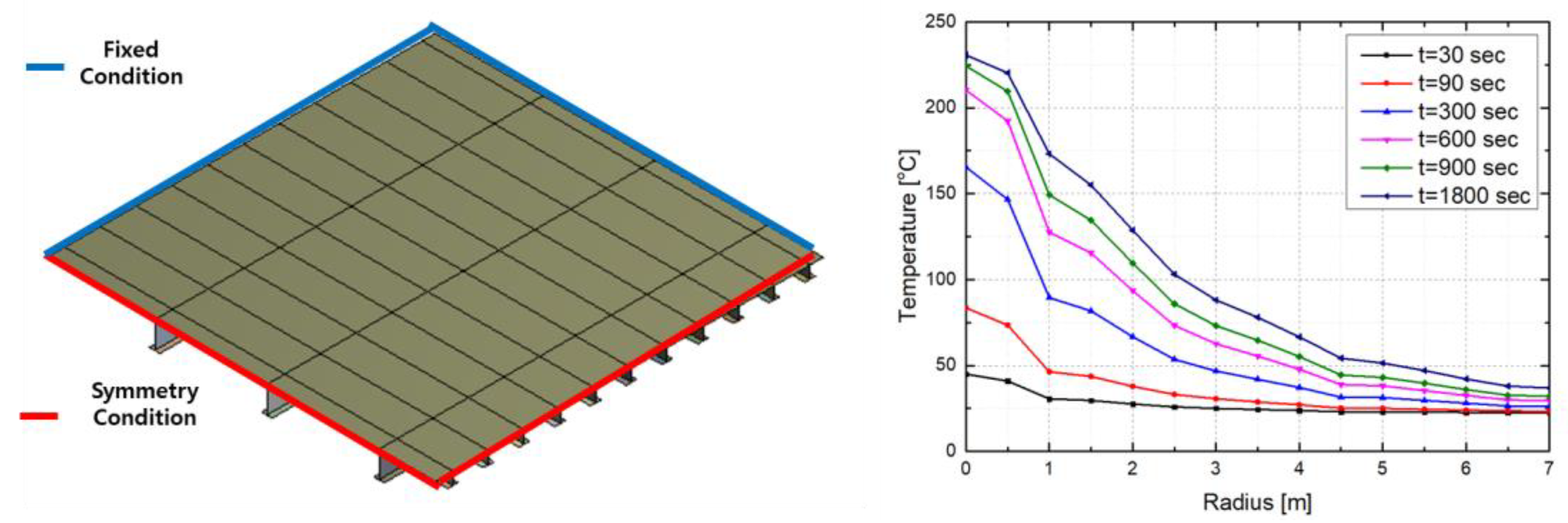
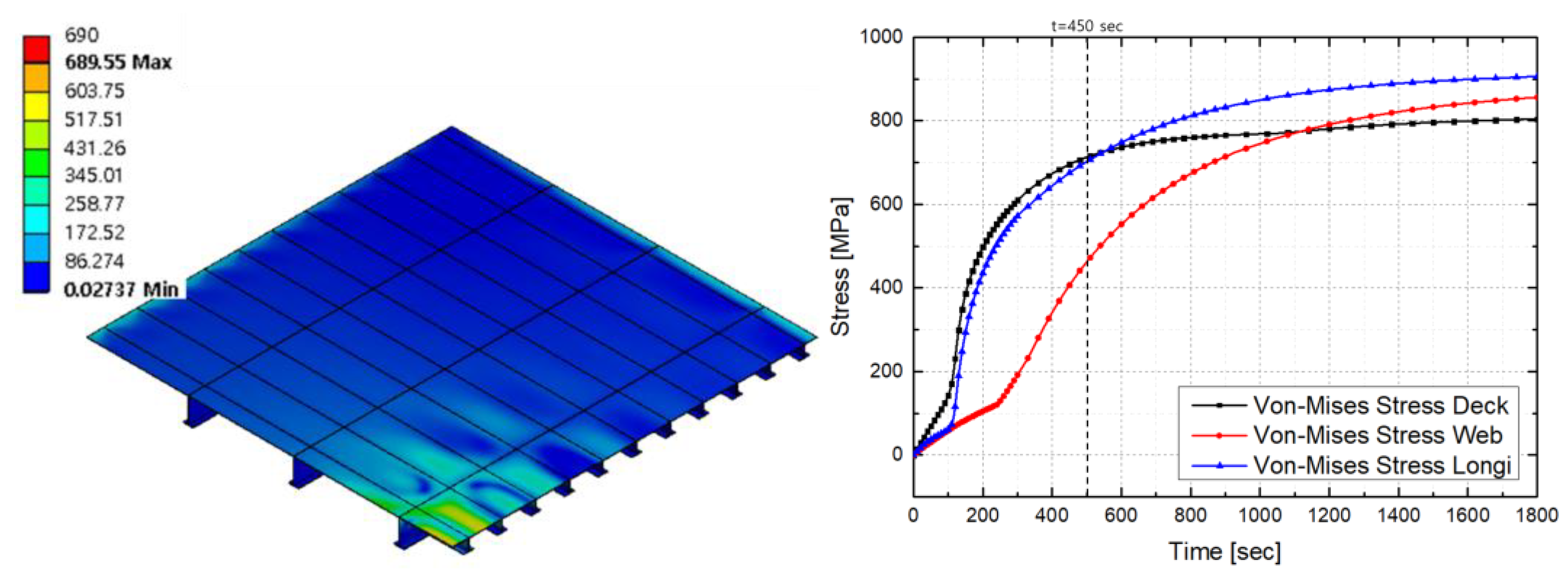
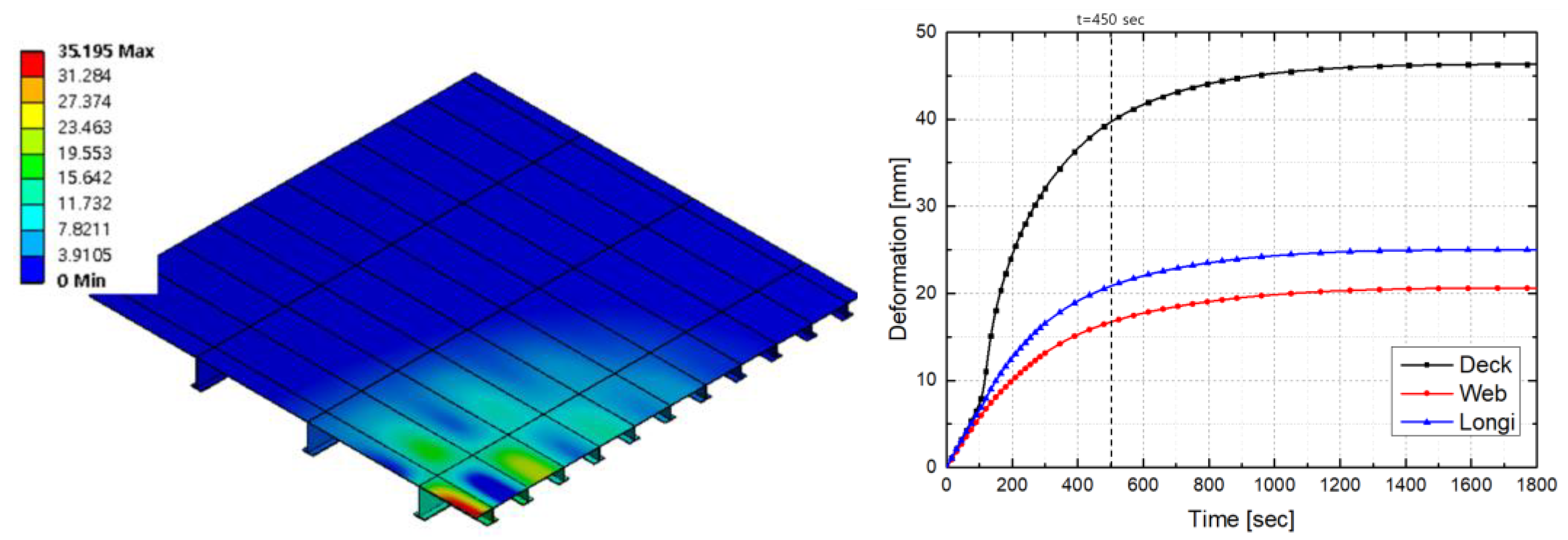
4.6. Transient Thermal-Structural Analysis

The thermal-structural analysis was performed with transient analysis, and a safe operation time was suggested based on the results. The thermal-structural analysis model is depicted in Figure 23 (left); the fixed condition was applied at the side edge. The temperature gradient was imported from heat transfer analysis to thermal-structural analysis. The distribution and history of deck temperature (Figure 23, right) are applied to the thermal-structural analysis. The material properties of a deck used to calculate the thermal stress are summarized in Table 8.
In this study, only the elastic properties were considered because the yield stress of the material was defined as a safety criterion. The contour and history of thermal stress and deformation results of the deck are depicted in Figure 24 and Figure 25. The yield stress was reached in approximately 450 s (7 min 30 s) at the center of a deck and the longitudinal frame in Table 9. As mentioned in the second section, the present study assumed that the exhaust gas was sprayed onto the deck while the VTOL was fixed in the landing state. Although this assumption overestimates the thermal stress of the deck, it is a conservative design condition to ensure the structural safety of the deck. In an actual VTOL operation, the time to reach the yield stress is expected to be more than 450 s because the height changes dynamically during take-off and landing. Therefore, it is necessary to estimate the exact time to reach the yield stress by considering the dynamically changing VTOL height through future study.

5. Conclusions

In this study, thermal flow analysis was performed to calculate the thermal load on the deck structure from the high-speed and high-temperature exhaust gas during landing and take-off. However, it was a physically unreasonable steady-state result because the coefficient of convection has a low value in the stagnation region. A reasonable convection coefficient was calculated using equivalent velocity based on the law of energy conservation considering the velocity and pressure. The heat transfer analysis was applied based on the thermal load conditions obtained from thermal flow analysis, and the temperature distribution and history were calculated. The temperature and convection coefficient distribution of exhaust gas were compared and verified with a real-scale experiment. Subsequently, the history of maximum temperature on the deck was verified again with the result. The results of thermal load were reasonable. Therefore, the distribution and history of temperature on the deck were applied to the thermal-structural analysis. Finally, this study suggested the time to reach the yield of the deck by the thermal stress and deformation from the thermal-structural analysis.

Author Contributions

J.-H.L. suggested the concept of thermal flow and stress analysis of processing VTOL system; S.-Y.H. analyzed the data and suggested an analysis procedure; H.-S.J. and S.-Y.H. performed a case study based on finite element analysis; H.-S.J. and J.-H.L. wrote the paper. All authors have read and agreed to the published version of the manuscript.

Funding

This research was funded by Defense Industry Technology Center (DITC) of Korea (Project code UC200005D).

Institutional Review Board Statement

Not applicable.

Informed Consent Statement

Not applicable.

Data Availability Statement

Not applicable.

Acknowledgments

This research was supported by Defense Industry Technology Center (DITC) of Korea (Project code UC200005D).

Conflicts of Interest

The authors declare no conflict of interest.

References

  1. Jambunathan, K.; Lai, E.; Moss, M.A.; Button, B.L. A review of heat transfer data for single circular jet impingement. Int. J. Heat Fluid Flow 1992, 13, 106–115. [Google Scholar] [CrossRef]
  2. Katti, V.; Prabhu, S.V. Experimental study and theoretical analysis of local heat transfer distribution between smooth flat surface and impinging air jet from a circular straight pipe nozzle. Int. J. Heat Mass Transf. 2008, 51, 4480–4495. [Google Scholar] [CrossRef]
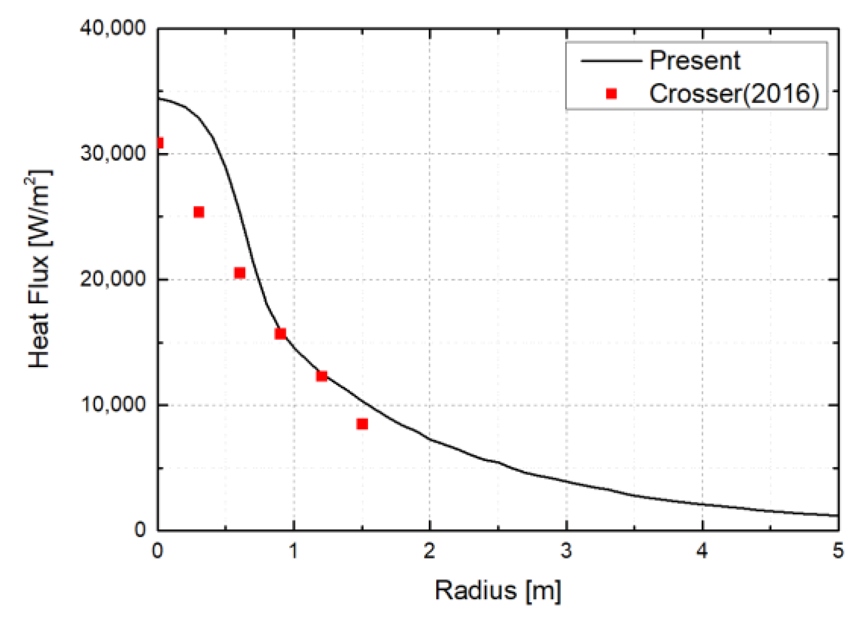
  3. Crosser, K.E. Heat Transfer Assessment of Aluminum Alloy Corrugated Naval Ship Deck Panels under VTOL Aircraft Thermal Loads. Ph.D. Dissertation, Virginia Polytechnic Institute and State University, Blacksburg, VA, USA, 2016. [Google Scholar]
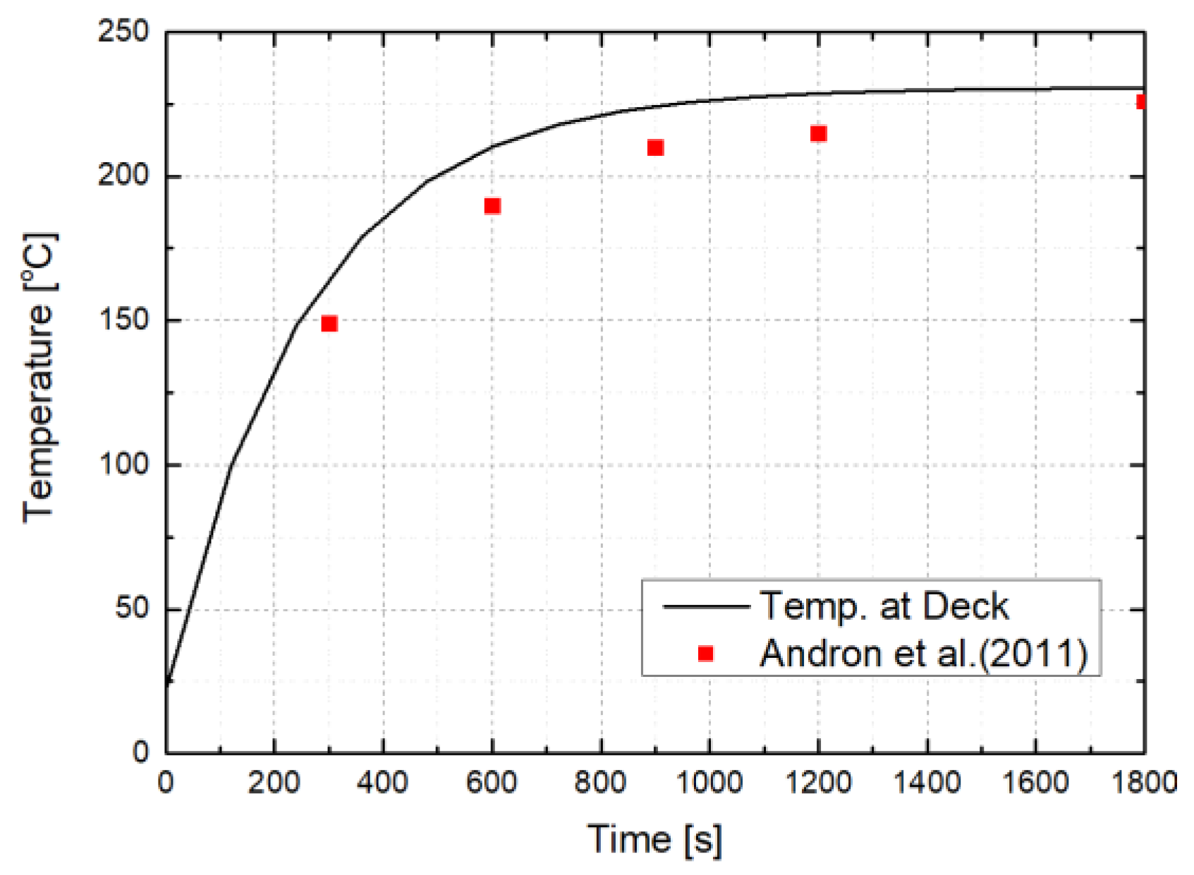
  4. Andron, P.; Conley, J.; Wells, B.; Erick, A. Land Based Testing of V-22 Osprey Aircraft for Deck Heating Effects—Test Results and Load Standardization; Naval Surface Warfare Center: Carderock, MD, USA, 2011. [Google Scholar]
  5. Zuckerman, N.; Lior, N. Jet Impingement Heat Transfer: Physics, Correlations, and Numerical Modeling. Adv. Heat Transf. 2006, 39, 565–631. [Google Scholar]
  6. Pattamatta, A.; Singh, G.; Mongia, H. Assessment of turbulence models for free and confined impinging jet flows. In Proceedings of the 42nd AIAA Thermophysics Conference, Honolulu, HI, USA, 27–30 June 2011; p. 3952. [Google Scholar]
  7. Barata, J.M. Fountain flows produced by multiple impinging jets in a crossflow. AIAA J. 1996, 34, 2523–2530. [Google Scholar] [CrossRef]
  8. Matsumoto, R.; Ishihara, I.; Yabe, T.; Ikeda, K.; Kikkawa, S.; Senda, M. Impingement heat transfer within arrays of circular jets including the effect of crossflow (AJTE99-6386). In Proceedings of the 5th ASME/JSME Thermal Engineering Joint Conference, San Diego, CA, USA, 14–19 March 1999; pp. 1–8. [Google Scholar]
  9. Gauntner, J.W. Survey of Literature on Flow Characteristics of a Single Turbulent Jet Impinging on a Flat Plate; National Aeronautics and Space Administration, Lewis Research Center: Washington, DC, USA, 1970. [Google Scholar]
  10. Martin, M.J.; Boyd, I.D. Stagnation-point heat transfer near the continuum limit. AIAA J. 2009, 47, 283–285. [Google Scholar] [CrossRef]
  11. Rao, S.R.; Srinath, S.; Bhargavi, V.; Dere, B.R. Analysis of Vertical Take-off Landing Aircraft using CFD. Int. J. Eng. Res. Technol. 2014, 3, 250–263. [Google Scholar]
  12. Annaswamy, A.; Choi, J.J.; Sahoo, D.; Egungwu, O.; Lou, H.; Alvi, F. Active-adaptive control of acoustic resonances in supersonic impinging jets. In Proceedings of the 33rd AIAA Fluid Dynamics Conference and Exhibit, Orlando, FL, USA, 23–26 June 2003; p. 3565. [Google Scholar]
  13. Choi, J.J.; Annaswamy, A.; Egungwu, O.; Alvi, F. Active noise control of supersonic impinging jet using pulsed microjets. In Proceedings of the 43rd AIAA Aerospace Sciences Meeting and Exhibit, Reno, NV, USA, 10–13 January 2005; p. 798. [Google Scholar]
  14. Beltaos, S.; Rajaratnam, N. Impinging circular turbulent jets. J. Hydraul. Div. 1974, 100, 1313–1328. [Google Scholar] [CrossRef]
  15. Beltaos, S.; Rajaratnam, N. Impingement of axisymmetric developing jets. J. Hydraul. Res. 1977, 15, 311–326. [Google Scholar] [CrossRef]
  16. Rajaratnam, N. Turbulent Jets; Elsevier: Amsterdam, The Netherlands, 1976. [Google Scholar]
  17. Nawani, S.; Subhash, M. A review on multiple liquid jet impingement onto flat plate. Mater. Today Proc. 2021, 46, 11190–11197. [Google Scholar] [CrossRef]
  18. O’Donovan, T.S.; Murray, D.B. Jet impingement heat transfer–Part I: Mean and root-mean-square heat transfer and velocity distributions. Int. J. Heat Mass Transf. 2007, 50, 3291–3301. [Google Scholar] [CrossRef]
  19. O’Donovan, T.S.; Murray, D.B. Jet impingement heat transfer–Part II: A temporal investigation of heat transfer and local fluid velocities. Int. J. Heat Mass Transf. 2007, 50, 3302–3314. [Google Scholar] [CrossRef]
  20. Han, B.; Goldstein, R.J. Jet-impingement heat transfer in gas turbine systems. Ann. N. Y. Acad. Sci. 2001, 934, 147–161. [Google Scholar] [CrossRef] [PubMed]
  21. Maghrabie, H.M. Heat transfer intensification of jet impingement using exciting jets-A comprehensive review. Renew. Sustain. Energy Rev. 2021, 139, 110684. [Google Scholar] [CrossRef]
  22. Vlachopoulos, J.; Tomich, J.F. Heat transfer from a turbulent hot air jet impinging normally on a flat plate. Can. J. Chem. Eng. 1971, 49, 462–466. [Google Scholar] [CrossRef]
  23. Olsson, E.E.M.; Ahrne, L.M.; Trägårdh, A.C. Heat transfer from a slot air jet impinging on a circular cylinder. J. Food Eng. 2004, 63, 393–401. [Google Scholar] [CrossRef]
  24. Parida, P.R.; Ekkad, S.V.; Ngo, K. Experimental and numerical investigation of confined oblique impingement configurations for high heat flux applications. Int. J. Therm. Sci. 2011, 50, 1037–1050. [Google Scholar] [CrossRef]
  25. Angioletti, M.; Di Tommaso, R.M.; Nino, E.; Ruocco, G. Simultaneous visualization of flow field and evaluation of local heat transfer by transitional impinging jets. Int. J. Heat Mass Transf. 2003, 46, 1703–1713. [Google Scholar] [CrossRef]
  26. Angioletti, M.; Nino, E.; Ruocco, G. CFD turbulent modelling of jet impingement and its validation by particle image velocimetry and mass transfer measurements. Int. J. Therm. Sci. 2005, 44, 349–356. [Google Scholar] [CrossRef]
  27. Achari, A.M.; Das, M.K. Application of various RANS based models towards predicting turbulent slot jet impingement. Int. J. Therm. Sci. 2015, 98, 332–351. [Google Scholar] [CrossRef]
  28. Coussirat, M.; Van Beeck, J.; Mestres, M.; Egusguiza, E.; Buchlin, J.M.; Escaler, X. Computational fluid dynamics modeling of impinging gas-jet systems: I. assessment of eddy viscosity models. J. Fluids Eng. 2005, 127, 691–703. [Google Scholar] [CrossRef]
  29. Coussirat, M.; Van Beeck, J.; Mestres, M.; Egusquiza, E.; Buchlin, J.M.; Valero, C. Computational fluid dynamics modeling of impinging gas-jet systems: II. Application to an industrial cooling system device. J. Fluids Eng. 2005, 127, 704–713. [Google Scholar] [CrossRef]
  30. Versteeg, H.K.; Malalasekera, W. An Introduction to Computational Fluid Dynamics: The Finite Volume Method; Pearson Education: London, UK, 2007. [Google Scholar]
  31. Hwang, C.B.; Lin, C.A. Improved low-reynolds-number ke model based on direct numerical simulation data. AIAA J. 1998, 36, 38–43. [Google Scholar] [CrossRef]
  32. Bolkcom, C. V-22 Osprey Tilt-Rotor Aircraft; Library of Congress Washington DC Congressional Research Service: Washington, DC, USA, 2004. [Google Scholar]
  33. Benson, T. Turboprop Thrust. Retrieved from NASA. 2006. Available online: http://www.grc.nasa.gov/www/K-12/airplane/turbprp.html (accessed on 24 December 2021).
  34. Rotaru, C.; Todorov, M. Helicopter Flight Physics; Flight Physics-Models, Techniques and Technologies, Defense Acquisition University: Fort Belvoir, VA, USA, 2018. [Google Scholar]
  35. Newman, S. Foundations of Helicopter Flight; Elsevier: Amsterdam, The Netherlands, 1994. [Google Scholar]
  36. Ansys Inc. Ansys® CFX Theory Guide; Ansys Inc.: Canonsburg, PA, USA, 2017. [Google Scholar]
  37. Hannat, R.; Morency, F. Numerical Validation of Conjugate Heat Transfer Method for Anti-/De-Icing Piccolo System. J. Aircr. 2014, 51, 104–116. [Google Scholar] [CrossRef]
  38. Park, T.H.; Choi, H.G.; Yoo, J.Y.; Kim, S.J. Streamline upwind numerical simulation of two-dimensional confined impinging slot jets. Int. J. Heat Mass Transf. 2003, 46, 251–262. [Google Scholar] [CrossRef]
  39. Heyerichs, K.; Pollard, A. Heat transfer in separated and impinging turbulent flows. Int. J. Heat Mass Transf. 1996, 39, 2385–2400. [Google Scholar] [CrossRef]
  40. Bejan, A. Convection Heat Transfer; John Wiley & Sons: Hoboken, NJ, USA, 2013. [Google Scholar]
  41. Commander, Naval Air Systems Command. NATOPS Flight Manual Navy Model MV-22B Tiltrotor; Change 58; NAVAIR: Patuxent River, MD, USA, 2006. [Google Scholar]
  42. Wadley, H.N.G.; Haj-Hariri, H.; Zok, F.; Norris, P.M. Multifunctional Thermal Management System and Related Method. USA Patent No. 10,107,560, 23 October 2018. [Google Scholar]
Figure 1. Schematic view of VTOL operation on naval vessel deck.
Jmse 10 00260 g001
Figure 2. Schematic diagram of the flow region of a circular impinging jet.
Jmse 10 00260 g002
Figure 3. Analysis procedure of VTOL on a naval vessel deck.
Jmse 10 00260 g003
Figure 4. Schematic turboprop engine operation.
Jmse 10 00260 g004
Figure 5. Schematic diagram of VTOL on the deck.
Jmse 10 00260 g005
Figure 6. Simulation model geometry in the computational domain. (left) Top view (right) Side view.
Jmse 10 00260 g006
Figure 7. The computational domain Summary. (left) Boundary condition (right) Mesh.
Jmse 10 00260 g007
Figure 8. Velocity section contour (left) and distribution (right) of the exhaust gas.
Jmse 10 00260 g008
Figure 9. Velocity vector (left) and streamline (right) of the exhaust gas.
Jmse 10 00260 g009
Figure 10. Convection coefficient location (left) and distribution (right) on the upper surface.
Jmse 10 00260 g010
Figure 11. Volume fraction contour (left) and distribution (right) of exhaust gas.
Jmse 10 00260 g011
Figure 12. Temperature (left) and pressure (right) distribution by radius.
Jmse 10 00260 g012
Figure 13. Temperature contour distribution of the exhaust gas. Top view (left) and section view (right).
Jmse 10 00260 g013
Figure 14. Pressure contour distribution of the exhaust gas. Top view (left) and section view (right).
Jmse 10 00260 g014
Figure 15. Convection coefficient contour (left) and distribution (right) on the impinging wall.
Jmse 10 00260 g015
Figure 16. Local Reynolds number (left) and Nusselt number (right) distribution.
Jmse 10 00260 g016
Figure 17. Calibrated convection coefficient distribution by radius (deck).
Jmse 10 00260 g017
Figure 18. Comparison of experimental and numerical convection coefficient (left) and temperature (right).
Jmse 10 00260 g018
Figure 19. Comparison of experimental and numerical heat flux.
Jmse 10 00260 g019
Figure 20. Simulation model of the heat transfer and thermal structure (deck).
Jmse 10 00260 g020
Figure 21. Distribution (left) and history (right) of temperature on the deck.
Jmse 10 00260 g021
Figure 22. Comparison of experimental and numerical maximum temperature history on the deck.
Jmse 10 00260 g022
Figure 23. Boundary conditions of thermal-structural analysis (left) and temperature distribution and history (right).
Jmse 10 00260 g023
Figure 24. Stress distribution (left) and history (right) of the deck structure.
Jmse 10 00260 g024
Figure 25. Deformation distribution (left) and history (right) of the deck structure.
Jmse 10 00260 g025
Table 1. Regions of the impingement wall.
RegionStagnation RegionTransition RegionWall Jet Region
Section 0 < r / D 1 1 < r / D 2.5 2.5 < r / D
Table 2. Empirical constants for the standard k-ε model.
ParameterValue
C μ 0.09
σ k 1.0
σ ε 1.3
C ε 1 1.44
C ε 2 1.92
Table 3. Simulation model geometry.
SpecificationValue
Weight24,950 (kg)
Nozzle   Diameter   ( D nozzle )0.9 (m)
Nozzle - to - Plate   ( H nozzle )1.32 (m)
Propeller   Diameter   ( D rortor )11.6 (m)
Propeller - to - Plate   ( H rortor )6.1 (m)
Length of simulation mode10 (m)
Table 4. Simulation model summary.
Analysis ModelDescription
Analysis TypeSteady state
DomainExhaust gas and air
Multiphase ModelHomogeneous model
Turbulence ModelStandard k-ε
Initial ConditionTemperature: 25 (℃)
VF (volume fraction): Air (1.0), exhaust gas (0.0)
Boundary Condition
(Inlet and Outlet)
Inlet condition: Exhaust nozzle
- Velocity: 105 (m/s)
- Temperature: 260 (℃)
- VF (Volume fraction): Exhaust gas (1.0), Air (0.0)
Inlet condition: Propeller
- Velocity: 21.2 (m/s)
- Temperature: 25 (℃)
- VF (volume fraction): Exhaust gas (0.0), Air (1.0)
Outlet: Opening condition
Table 5. Convergence of temperature and velocity using grid refinement.
Grid Size (mm)T [K]V (m/s)
ValueDifferenceValueDifference
200537.796-81.451
180538.5850.15%86.2075.84%
150538.8920.06%88.7072.90%
120539.6430.14%92.7174.52%
100539.8740.04%94.2591.66%
80539.9740.02%95.1660.96%
50540.0070.01%95.5040.36%
Table 6. Summary of heat transfer analysis.
SpecificationValue
Thickness of deck0.013 (m)
Initial Temperature25 (°C)
Forced convection by Impinging Jet h e x ( r ) ,   T e x ( r ) depicted in Figure 15
Natural   convection   by   Ambient   ( h a ) 5   ( W / m 2 K )
Ambient   Temperature   ( T ) 22 (°C)
Analysis time1800 (s)
Table 7. Material properties of HY 100.
Material PropertyValue
Density 7744   ( kg / m 3 )
Specific Heat407 (J/kg∙K)
Thermal Conductivity34 (W/m∙K)
Table 8. Deck material properties.
Material PropertyValue
Elastic Modulus207 (GPa)
Poisson’s Ratio0.3
Yield Stress690 (MPa)
Thermal Expansion Coefficient1.4 × 10−5 (1/K)
Table 9. Thermal-structural analysis results.
Structural MemberArrival Time at Yield Stress
Deck450 (s)
Web frame810 (s)
Longitudinal450 (s)
Publisher’s Note: MDPI stays neutral with regard to jurisdictional claims in published maps and institutional affiliations.

