Neural Network Non-Singular Terminal Sliding Mode Control for Target Tracking of Underactuated Underwater Robots with Prescribed Performance

Abstract

This paper proposes a neural network-based nonsingular terminal sliding mode controller with prescribed performances for the target tracking problem of underactuated underwater robots. Firstly, the mathematical formulation of the target tracking problem is presented with an underactuated underwater robot model and the corresponding control objectives. Then, the target tracking errors from the line-of-sight guidance law are transformed using the prescribed performance technique to achieve good dynamic performance and steady-state performance that meet the pre-set conditions. Meanwhile, considering the model’s uncertainties and the external disturbances to the underwater robots, a target tracking controller is proposed based on the radial basis function (RBF) neural network and the non-singular terminal sliding mode control. Lyapunov stability analysis and homogeneity theory prove the tracking errors can converge on a small region that contains the origin with prescribed performance in finite time. In the simulation comparison, the controller proposed in this paper had better dynamic performance, steady-state performance and chattering supression. In particular, the steady-state error of the tracking error was lower, and the convergence time of the tracking error in the vertical distance was reduced by 19.1%.

1. Introduction

In recent years, underwater robots have been widely used in various underwater tasks. Typical applications include search and rescue, monitoring and surveillance, petroleum exploration, deep-sea archaeological research, ship hull maintenance industry [1,2,3] and so on. In the underwater applications mentioned above, underwater robots are often required to track the targets in a fast and accurate manner. As underwater robots generally have the characteristics of many uncertainties, high nonlinearity and strong coupling dynamics, and work in an environment with unknown external disturbances, it is typically difficult for traditional linear controllers to achieve good tracking control performance.

Many advanced control methods have been used in the control of underwater robots, such as backstepping control [4,5,6], model predictive control [7,8], neural network control [9,10,11,12,13], active disturbance rejection control [14,15,16], sliding mode control [17,18,19,20,21,22,23], adaptive and distributed control [24,25,26] and reinforcement learning [27,28,29,30]. In the above methods, sliding mode control has been widely studied or used because of its strong robustness to the external time-varying disturbance and unmodeled characteristics, fast responses and easy implementation. Yingkai Xia et al. designed of an improved line-of-sight-based adaptive sliding mode tracking controller for highly coupled dynamics, ocean current disturbances and input saturation of underactuated autonomous underwater vehicles (AUVs) [21]. For the problems of the remote operated vehicle (ROV) movement instability and large tracking error caused by unknown disturbances, an adaptive sliding mode motion controller was developed by Zongsheng Wang et al. [20]. However, the standard sliding mode control can only realize the asymptotic stability of the system, and cannot guarantee the convergence time. As an effective method to speed up the convergence of tracking errors, terminal sliding mode control achieves finite-time stability by introducing fractional order terms when constructing a sliding hyperplane. For underactuated underwater vehicles, Taha Elmokadem et al. designed a target tracking controller based on terminal sliding mode control, and proved that the tracking errors can converge to zero within a specified finite time [18]. However, the negative fractional power terms contained in the controller may lead to a singularity when the errors converge. Cao Jian et al. designed a non-singular terminal sliding mode controller that evades the issue of a singularity in the target tracking problem of underwater robots [31]. Nevertheless, it is necessary to obtain the upper bound of uncertainty in advance. Strong robustness can be obtained by setting a larger switching gain. However, this will lead to a serious chattering problem, affect the control accuracy and increase the energy consumption, which are harmful to the tracking control of underwater robots. B.M. Patre et al. added a state observer to the sliding mode controller to reduce the switching gains [19], thereby attenuating the chattering. The precondition of applying this method is that the uncertainty changes slowly and the first derivative is almost zero, which is inconsistent with the actual working environment of underwater robots. In practice, underwater robots are always subject to various uncertainties, such as unknown parameters, unmodeled time-varying dynamics and measurement noise. A neural network can approximate nonlinear time-varying functions and has been becoming one of the most effective ways to observe uncertainties [9,12,13]. It is worth noting that a neural network can reduce the switching gain of a sliding mode controller by approximating unmodeled uncertainties. Therefore, a terminal sliding mode controller combined with RBF neural network technology improves the tracking control performance while attenuating chattering.

As underwater tasks are becoming more complex, it is important to ensure good target tracking of underwater robots. While improving the robustness to external disturbances and modeling uncertainties, the controller should also pay attention to the dynamic performance and steady-state performance of the tracking errors. The performance control parameters proposed by Charalampos P. Bechlioulis et al. include constraints to limit errors, which not only ensures that the steady-state errors are always less than a pre-set boundary, but also limits the dynamic performance of the system state errors, including convergence rate and overshoot, to meet the pre-set conditions [32]. Charalampos P. Bechlioulis et al. developed an approximation-free trajectory tracking controller for underactuated AUVs with prescribed performances [33]. Nevertheless, this controller ignored the existence of external disturbances and modeling uncertainties. Omid Elhaki et al. created a neural network-based target tracking controller for an underactuated AUV with a prescribed performance to overcome unmodeled dynamics and external disturbances [10]. The prescribed performance technique is applied to trajectory tracking to prevent collisions and improve control performance [34,35]. Furthermore, a finite-time performance function [36] and a nonlogarithmic piecewise error mapping function [37] have also been introduced to accelerate convergence. However, the finite-time convergence of the controllers has not been investigated in detail.

Differently from previous research, in order to achieve robustness to uncertainties and external disturbances, realize finite-time convergence, attenuate chattering and obtain the tracking error’s prescribed performance simultaneously, this paper proposes a neural network nonsingular terminal sliding mode controller with prescribed performance for the target tracking problem of underactuated underwater robots. Compared with the nonsingular terminal sliding mode controller, the proposed controller has obvious advantages in dynamic performance and steady-state performance. Additionally, its chattering is weaker than that of a nonsingular terminal sliding mode controller with prescribed performances. Firstly, the mathematical formulation of the target tracking problem is proposed for the underactuated underwater robot model and the corresponding control objectives. The target tracking guidance law is designed based on the line-of-sight. The range and bearing angles of the robot relative to the target are obtained as tracking errors. Then, the range and bearing angles are transformed into corresponding transformation errors with prescribed performances. The tracking errors converge to arbitrarily small limit bounds, and the dynamic performance is optimized with a prespecified maximum overshoot and the convergence speed. The non-singular terminal sliding mode controller was developed to ensure that the underwater robot is robust to external disturbances and modeling uncertainties, and guarantee finite-time convergence of the tracking errors. For improving the accuracy of tracking control and attenuating the chattering of sliding mode control, an RBF neural network estimator is integrated to approximate modeling uncertainties. Finally, a Lyapunov stability synthesis and homogeneity theory show that the tracking errors converge in finite time on a small region that contains zero with the prescribed performance. In the simulation comparison, the controller proposed in this paper had better dynamic performance, steady-state performance and chattering suppression.

The remainder of this paper is ordered as follows. In Section 2, the formulation of the target tracking problem for underwater robots is stated. In Section 3, the design of the neural network nonsingular terminal sliding mode controller with prescribed performance and its stability analysis are presented. Section 4 reports simulation experiments and performance comparisons. Finally, Section 5 draws the conclusions and proposes future research.

2. Problem

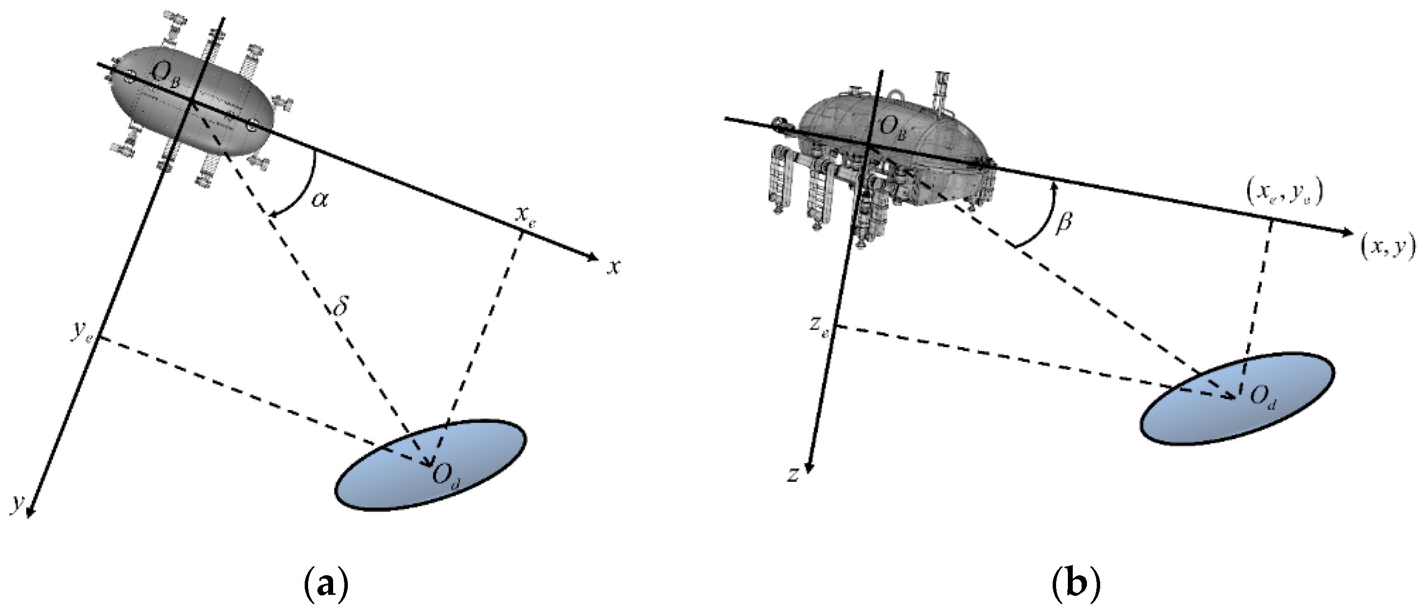
2.1. Underwater Robot Model

As shown in Figure 1, the motion of underwater robots is commonly described with the use of two coordinate systems. The first is the geotectonic inertial reference coordinate system {I}: the axes of the coordinate system are fixed to the earth and the origin is selected somewhere on the ground. The other is the body reference coordinate system {B}, whose origin coincides with the buoyancy center of the underwater robot. The robot is self-stable under roll, so the motion model does not need to consider this degree of freedom. The kinematic model of the underwater robot is described by the following equation:

$$\left[\begin{array}{l}\dot{\xi }\hfill \\ \dot{\eta }\hfill \\ \dot{\zeta }\hfill \\ \dot{\theta }\hfill \\ \dot{\psi }\hfill \end{array}\right]=\left[\begin{array}{lllll}\cos \psi \cos \theta \hfill & -\sin \psi \hfill & \sin \theta \cos \psi \hfill & 0\hfill & 0\hfill \\ \sin \psi \cos \theta \hfill & \cos \psi \hfill & \sin \theta \sin \psi \hfill & 0\hfill & 0\hfill \\ -\sin \theta \hfill & 0\hfill & \cos \theta \hfill & 0\hfill & 0\hfill \\ 0\hfill & 0\hfill & 0\hfill & 1\hfill & 0\hfill \\ 0\hfill & 0\hfill & 0\hfill & 0\hfill & \raisebox{1ex}{$1$}\!\left/ \!\raisebox{-1ex}{$\cos \theta $}\right.\hfill \end{array}\right]\left[\begin{array}{l}u\hfill \\ v\hfill \\ w\hfill \\ q\hfill \\ r\hfill \end{array}\right]$$

(1)

where $\xi$, $\eta$ and $\zeta$ indicate the position in {I}; $\theta$ represents the pitch angle in {I}; and $\psi$ represents the yaw angle in {I}. $u$, $v$, $w$, $q$ and $r$ indicate the surge, sway, heave, pitch and yaw velocities in {B}.

By applying the Newton–Euler formulation, the dynamics of the underwater robot in {B} can be described as [38]:

$$M\dot{v}+C\left(v\right)v+D\left(v\right)v+G\left(\eta \right)={\tau }_{ex}+{\tau }_v$$

(2)

where $M\in R^{5\times 5}$ is the inertia matrix that includes body mass and added mass; $C\in R^{5\times 5}$ is a matrix describing centripetal and Coriolis forces produced due to added inertia; $D\in R^{5\times 5}$ represents the hydrodynamic damping matrix; $G\left(\eta \right)\in R^5$ represents the combined gravitational and buoyancy forces vector; ${\tau }_{ex}\in R^5$ is the unknown time-varying vector of external disturbance forces such as waves and ocean current; and ${\tau }_v\in R^5$ is s the vector of control moments and forces.

Due to the complexity and variability of the actual marine environment, it is difficult to ensure the accuracy of the hydrodynamic parameters obtained from an experiment, so the parameters are still uncertain. Therefore, $M$, $C\left(v\right)$ and $D\left(v\right)$ can be divided into two parts: the nominal dynamics $M_0$, $C_0\left(v\right)$ and $D_0\left(v\right)$; and dynamic uncertainties $\Delta M$, $\Delta C$ and $\Delta D$:

$$\begin{array}{l}M=M_0+\Delta M\\ C\left(v\right)=C_0(v)+\Delta C\left(v\right)\\ D\left(v\right)=D_0(v)+\Delta D\left(v\right)\end{array}$$

(3)

Then, the dynamic equation can be rewritten as the following form:

$$M_0\dot{v}+C_0\left(v\right)v+D_0\left(v\right)v+G\left(\eta \right)+\Delta ={\tau }_{ex}+{\tau }_v$$

(4)

where $\Delta =\Delta M+\Delta C+\Delta D={\left[{\Delta }_u,{\Delta }_v,{\Delta }_w,{\Delta }_q,{\Delta }_r\right]}^T$ is the total uncertainty of the dynamics.

Finally, for convenience of controller design, the kinematics model and dynamics model of an underwater robot are presented in the standard form of a nonlinear system in Equation (5):

$$\{\begin{array}{l} {\dot{x}}_1=A{x}_2\hfill \\ {\dot{x}}_2=f\left(x,t\right)+g\left(t\right)u\left(t\right)+{\Delta }^{\prime }\left(x,t\right)+d\left(t\right)\hfill \end{array}$$

(5)

where $x={\left[x_1,x_2\right]}^T$ is the state variable of the system, and its expression is:

$$\begin{array}{l}{x}_1={\left[\xi ,\eta ,\zeta ,\theta ,\psi \right]}^T\\ x_2={\left[u,v,w,q,r\right]}^T\end{array}$$

(6)

The controller input $u\left(t\right)$ is expressed as:

$$u\left(t\right)={\tau }_v={\left[T_u,T_v,T_w,T_q,T_r\right]}^T$$

(7)

The limits of control moments and forces are −6000 to 6000 N(Nm). Since there is no thruster actuator in the $Y$ direction, $T_v\equiv 0$.$f\left(x,t\right)$ is a smooth nonlinear term, and it can be expressed according to Equation (2):

$$f(x,t)=-M_0^{-1}\left[C_0\left(x_2\right)x_2+D_0\left(x_2\right)x_2+G\left(x_1\right)\right]={\left[f_u,f_v,f_w,f_q,f_r\right]}^T$$

(8)

The invertible matrix $g\left(t\right)$ is the control gain function. ${\Delta }^{\prime }\left(x,t\right)$ is the model uncertainty function; $d\left(t\right)$ is the external bounded disturbance function:

$$\begin{array}{l}g\left(t\right)=M_0^{-1}=diag\left\{g_u,g_v,g_w,g_q,g_r\right\}\\ {\Delta }^{\prime }\left(x,t\right)=-M_0^{-1}\Delta ={\left[-g_u{\Delta }_u,-g_v{\Delta }_v,-g_w{\Delta }_w,-g_q{\Delta }_q,-g_r{\Delta }_r\right]}^T\\ d\left(t\right)=M_0^{-1}{\tau }_{ex}={\left[{{\tau }^{\prime }}_{ex1},{{\tau }^{\prime }}_{ex2},{{\tau }^{\prime }}_{ex3},{{\tau }^{\prime }}_{ex4},{{\tau }^{\prime }}_{ex5}\right]}^T\end{array}$$

(9)

2.2. Control Objectives

The position error between the underwater robot and the tracking target can be formulated as follows:

$$\left[\begin{array}{c}{x}_e\\ y_e\\ z_e\end{array}\right]=\left[\begin{array}{ccc}\cos \psi \cos \theta & \sin \psi \cos \theta & -\sin \theta \\ -\sin \psi & \cos \psi & 0\\ \sin \theta \cos \psi & \sin \theta \sin \psi & \cos \theta \end{array}\right]\left[\begin{array}{c}{\xi }_d-{\xi }_B\\ {\eta }_d-{\eta }_B\\ {\zeta }_d-{\zeta }_B\end{array}\right]$$

(10)

In Equation (10), $({\xi }_B,{\eta }_B,{\zeta }_B)$ and $({\xi }_d,{\eta }_d,{\zeta }_d)$ are the coordinates of the underwater robot and the tracking target in {I} respectively. The transformation relationship between the range and bearing angles $(\delta ,\beta ,\alpha ,Z_e)$ and $(x_e,y_e,z_e)$ is as follows:

$$\{\begin{array}{l}\delta =\sqrt{x_e{}^2+y_e{}^2}\hfill \\ \beta =-\arctan (z_e/\sqrt{x_e{}^2+y_e{}^2})\hfill \\ \alpha =\arctan (y_e/x_e)\hfill \\ Z_e=z_e\hfill \end{array}$$

(11)

and

$$\{\begin{array}{l}{x}_e=\delta \cos \alpha \hfill \\ y_e=\delta \sin \alpha \hfill \\ z_e=Z_e\hfill \end{array}$$

(12)

The range and bearing angles $(\delta ,\beta ,\alpha ,Z_e)$ are considered to be four tracking errors. Figure 2a is the horizontal projection of the underwater robot and the target from the top view perspective in {B}. Figure 2b is the vertical plane projection of the underwater robot with the $z$ axis coplanar with the target in {B}. It can be seen that $\delta$ is the distance from the projection of the target on the $x{O}_{B}y$ plane to the $O_B$ point; $\alpha$ is the angle between the line projected by the target and the underwater robot on the $x{O}_{B}y$ plane and the $x$ axis; $Z_e$ is the distance from the $x{O}_{B}y$ plane to the target in {B}; and $\beta$ is the angle between the line of the underwater robot to the target and the $x{O}_{B}y$ plane, as shown in Figure 2.

Derivation of Equation (12) yields Equation (13):

$$\{\begin{array}{l}{\dot{x}}_e=-u-q{z}_e+r{y}_e+{\chi }_{1d}\hfill \\ {\dot{y}}_e=-v-r(x_e+z_e\tan \theta )+{\chi }_{2d}\hfill \\ {\dot{z}}_e=-w+q{x}_e+r{y}_e\tan \theta +{\chi }_{3d}\hfill \end{array}$$

(13)

where

$$\{\begin{array}{l}{\chi }_{1d}={\dot{\xi }}_d\cos \theta \cos \psi +{\dot{\eta }}_d\cos \theta \sin \psi -{\dot{\zeta }}_d\sin \theta \hfill \\ {\chi }_{2d}=-{\dot{\xi }}_d\sin \psi +{\dot{\eta }}_d\cos \psi \hfill \\ {\chi }_{3d}={\dot{\xi }}_d\sin \theta \cos \psi +{\dot{\eta }}_d\sin \theta \sin \psi +{\dot{\zeta }}_d\cos \theta \hfill \end{array}$$

(14)

By combining Equations (11)–(13), the dynamic error equation related to the $(\delta ,\beta ,\alpha ,Z_e)$ can be obtained as follows:

$$\{\begin{array}{l}\dot{\delta }=-u\cos \alpha -v\sin \alpha -q{Z}_e\cos \alpha -r{Z}_e\tan \theta \sin \alpha +{\chi }_{1d}\cos \alpha +{\chi }_{2d}\sin \alpha \hfill \\ \dot{\beta }=-\left[x_e\delta /\left({\delta }^2+Z_e{}^2\right)\right]q+Z_e\dot{\delta }/\left({\delta }^2+Z_e{}^2\right)-\left[\left(-w+r{y}_e\tan \theta +{\chi }_{3d}\right)/\left({\delta }^2+Z_e{}^2\right)\right]\delta \hfill \\ \dot{\alpha }=-\left[\left(Z_e\tan \theta \cos \alpha +\delta \right)/\delta \right]r+\left(u\sin \alpha -v\cos \alpha +q{Z}_e\sin \alpha -{\chi }_{1d}\sin \alpha +{\chi }_{2d}\cos \alpha \right)/\delta \hfill \\ {\dot{Z}}_e=-w+q{x}_e+r{y}_e\tan \theta +{\chi }_{3d}\hfill \end{array}$$

(15)

The control objectives of this paper include the following. By designing the controller input $u\left(t\right)$, the target tracking errors $(\delta ,\beta ,\alpha ,Z_e)$ stabilize near the origin in finite time with the pre-set dynamic responses and meet the steady-state error limit. To avoid collisions, a small positive threshold $\tilde{\delta }$ is introduced as the safe distance between the underwater robot and the target. Therefore, $\delta$ should converge to $\tilde{\delta }$, and the others should converge to zero. Moreover, the proposed controller is expected to be robust to the uncertainties of the dynamic model and unknown external disturbances, and can attenuate the chattering.

3. Controller Design

3.1. Prescribed Performance and Error Transformation

The prescribed performance is defined when the error can converge to a pre-assigned residual set; and the maximum overshoot, convergence rate and steady-state error in the convergent response strictly satisfy a bounded decreasing time function defined as the performance function [39]. The following formula is the mathematical expression of the prescribed performance.

$$L_1{\eta }_1<\delta <H_1{\eta }_1$$

(16)

$$-L_2{\eta }_2<\beta <H_2{\eta }_2$$

(17)

$$-L_3{\eta }_3<\alpha <H_3{\eta }_3$$

(18)

$$-L_4{\eta }_4<Z_e<H_4{\eta }_4$$

(19)

where, $H_1,L_1,H_2,L_2,H_3,L_3,H_4$ and $L_4$ are positive real numbers, and $H_1>L_1$ should be guaranteed. ${\eta }_i,i=1,2,3,4$ is called the performance function, which could govern the dynamic and steady state performances of the errors. It is defined as ${\eta }_i=\left({\eta }_{i0}-{\eta }_{i\infty }\right)e^{-a_{i}t}+{\eta }_{i\infty },i=1,2,3,4$ and ${\eta }_{i0}>{\eta }_{i\infty }>0,a_i>0$, where ${\eta }_{i\infty }$ should be sufficiently small positive real numbers. ${\eta }_{i\infty }$ determines the final boundaries of the tracking error. $a_i$ determines the convergence rate of the tracking errors, which is mainly related to the dynamic performance of the system. The prescribed performance and error transformation function are shown in Figure 3.

It can be seen in Equation (11) that when $\delta =0,\beta =\pm \pi /2$, a singularity will occur in the system. If $\alpha =\pm \pi /2$, since there is no actuator for the lateral direction of the underwater robot, the system will lose control in this direction. Therefore, the above situations should be avoided. Since $\beta ,\alpha$ and $Z_e$ represent the vertical tracking error, horizontal orientation tracking error and vertical distance between the underwater robot and the target, respectively, they shall converge to zero as $t\to \infty$. If $\beta ,\alpha ,Ze$ satisfy the constraints of Equations (17)–(19), the possible singularity can be avoided and the system can always be under control. Further, when the bound of Equation (16) is strictly satisfied, the horizontal distance error $\delta$ converges to the minimum safe distance such that $\delta (\infty )=\tilde{\delta }\ne 0$ as $t\to \infty$. This definition can not only eliminate the potential singularity of the system, but also maintain a safe distance between the robot and the tracking target.

It is difficult to deal with inequality constraints Equations (16)–(19) directly. Therefore, inequality constraints are firstly transformed into equality constraints, and four smooth and strictly increasing functions are defined as error transformation functions $f_1\left({\epsilon }_{\delta }\right),f_2\left({\epsilon }_{\beta }\right),f_3\left({\epsilon }_{\alpha }\right),f_4\left({\epsilon }_{Z_e}\right)$ with the following properties:

$${\delta }_{\left(t\right)}={\eta }_1{f}_1\left({\epsilon }_{\delta }\right),\hspace{1em}\hspace{1em}{\beta }_{\left(t\right)}={\eta }_2{f}_2\left({\epsilon }_{\beta }\right),\hspace{1em}\hspace{1em}{\alpha }_{\left(t\right)}={\eta }_3{f}_3\left({\epsilon }_{\alpha }\right),\hspace{1em}\hspace{1em}{Z}_{e\left(t\right)}={\eta }_4{f}_4\left({\epsilon }_{Z_e}\right),$$

(20)

$$L_1<f_1\left({\epsilon }_{\delta }\right)<H_1,\hspace{1em}\hspace{1em}-L_2<f_2\left({\epsilon }_{\beta }\right)<H_2,\hspace{1em}-L_3<f_3({\epsilon }_{\alpha })<H_3,\hspace{1em}-L_4<f_4\left({\epsilon }_{Z_e}\right)<H_4,$$

(21)

$$\underset{{\epsilon }_{\delta }\to +\infty }{\lim }{f}_1\left({\epsilon }_{\delta }\right)=H_1,\hspace{1em}\hspace{1em}\underset{{\epsilon }_{\beta }\to +\infty }{\lim }{f}_2\left({\epsilon }_{\beta }\right)=H_2,\hspace{1em}\hspace{1em}\underset{{\epsilon }_{\alpha }\to +\infty }{\lim }{f}_3\left({\epsilon }_{\alpha }\right)=H_3,\hspace{1em}\hspace{1em}\underset{{\epsilon }_{Z_e}\to +\infty }{\lim }{f}_4\left({\epsilon }_{\delta }\right)=H_4,$$

(22)

$$\underset{{\epsilon }_{\delta }\to -\infty }{\lim }{f}_1\left({\epsilon }_{\delta }\right)=L_1,\hspace{1em}\hspace{1em}\underset{{\epsilon }_{\beta }\to -\infty }{\lim }{f}_2\left({\epsilon }_{\beta }\right)=-L_2,\hspace{1em}\hspace{1em}\underset{{\epsilon }_{\alpha }\to -\infty }{\lim }{f}_3\left({\epsilon }_{\alpha }\right)=-L_3,\hspace{1em}\hspace{1em}\underset{{\epsilon }_{Z_e}\to -\infty }{\lim }{f}_4\left({\epsilon }_{\delta }\right)=-L_4,$$

(23)

$$f_1\left(0\right)=L_1+{\epsilon }_1,\hspace{1em}\hspace{1em}\hspace{1em}{f}_2\left(0\right)=0,\hspace{1em}\hspace{1em}\hspace{1em}{f}_3\left(0\right)=0,\hspace{1em}\hspace{1em}\hspace{1em}{f}_4\left(0\right)=0,$$

(24)

$$\underset{{\epsilon }_{\delta }\to 0}{\lim }\delta ={\eta }_1\left(L_1+{\epsilon }_1\right),\hspace{1em}\underset{{\epsilon }_{\beta }\to 0}{\lim }\beta =0,\hspace{1em}\hspace{1em}\hspace{1em}\underset{{\epsilon }_{\alpha }\to 0}{\lim }\alpha =0,\hspace{1em}\hspace{1em}\hspace{1em}\underset{{\epsilon }_{Z_e}\to 0}{\lim }{\mathrm{Z}}_e=0,$$

(25)

where ${\epsilon }_{\delta },{\epsilon }_{\beta },{\epsilon }_{\alpha }$ and ${\epsilon }_{Z_e}$ are defined as the transformation errors corresponding to tracking errors $\delta ,\beta ,\alpha ,Z_e$ respectively. When the transformation errors converge to zero, the tracking errors converge with prescribed dynamic and steady-state performances. $\beta ,\alpha ,Z_e$ converge to zero, and $\delta$ converges to the minimum safe distance $\tilde{\delta }=\underset{\begin{array}{l}{\epsilon }_{\delta }\to 0\\ t\to \infty \end{array}}{\lim }\delta ={\eta }_{1\infty }\left(L_1+{\epsilon }_1\right)$.

According to the above properties, $f_1\left({\epsilon }_{\delta }\right),f_2\left({\epsilon }_{\beta }\right),f_3\left({\epsilon }_{\alpha }\right),f_4\left({\epsilon }_{Z_e}\right)$ is designed as follows:

$$\{\begin{array}{l}{f}_1\left({\epsilon }_{\delta }\right)=\frac{H_1{e}^{\left(p_1{\epsilon }_{\delta }+v_1\right)}+L_1{e}^{-\left(p_1{\epsilon }_{\delta }+v_1\right)}}{e^{\left(p_1{\epsilon }_{\delta }+v_1\right)}+e^{-\left(p_1{\epsilon }_{\delta }+v_1\right)}}\hfill \\ f_2\left({\epsilon }_{\beta }\right)=\frac{H_2{e}^{\left(p_2{\epsilon }_{\beta }+v_2\right)}-L_2{e}^{-\left(p_2{\epsilon }_{\beta }+v_2\right)}}{e^{\left(p_2{\epsilon }_{\beta }+v_2\right)}+e^{-\left(p_2{\epsilon }_{\beta }+v_2\right)}}\hfill \\ f_3\left({\epsilon }_{\alpha }\right)=\frac{H_3{e}^{\left(p_3{\epsilon }_{\alpha }+v_3\right)}-L_3{e}^{-\left(p_3{\epsilon }_{\alpha }+v_3\right)}}{e^{\left(p_3{\epsilon }_{\alpha }+v_3\right)}+e^{-\left(p_3{\epsilon }_{\alpha }+v_3\right)}}\hfill \\ f_4\left({\epsilon }_{Z_e}\right)=\frac{H_4{e}^{\left(p_4{\epsilon }_{Z_e}+v_4\right)}-L_4{e}^{-\left(p_4{\epsilon }_{Z_e}+v_4\right)}}{e^{\left(p_4{\epsilon }_{Z_e}+v_4\right)}+e^{-\left(p_4{\epsilon }_{Z_e}+v_4\right)}}\hfill \end{array}$$

(26)

where $v_1=0.5\ln \left({\epsilon }_1/\left(H_1-L_1-{\epsilon }_1\right)\right)$, $v_2=0.5\ln \left(H_2/L_2\right)$, $v_3=0.5\ln \left(H_3/L_3\right)$, $v_4=0.5\ln \left(H_4/L_4\right)$ and ${\epsilon }_1>0,p_i>0,i=1,2,3,4$.

The tracking errors should initially satisfy $L_1{\eta }_{10}<\delta \left(0\right)<H_1{\eta }_{10}$, $-L_2{\eta }_{20}<\beta \left(0\right)<H_2{\eta }_{20}$, $-L_3{\eta }_{30}<\alpha \left(0\right)<H_3{\eta }_{30}$ and $-L_4{\eta }_{40}<Z_e\left(0\right)<H_4{\eta }_{40}$; that is, $H_1,H_2,H_3,H_4,L_2,L_3,L_4$ should be sufficiently large positive numbers, $L_1$ should be a small enough positive number and ${\epsilon }_{\delta },{\epsilon }_{\beta },{\epsilon }_{\alpha },{\epsilon }_{Z_e}\in L_{\infty }$. Thus, the tracking errors of the system can be guaranteed to meet the prescribed performance. All the signals of the closed-loop system are bounded and non-singular, and the tracking errors converge with the specified dynamic and steady state performance (i.e., maximum overshoot, convergence rate and final accuracy). Finally, the tracking errors would be stabilized in the pre-set boundary: $L_1{\eta }_{1\infty }<\delta (\infty )<H_1{\eta }_{1\infty }$, $-L_2{\eta }_{2\infty }<\beta (\infty )<H_2{\eta }_{2\infty }$, $-L_3{\eta }_{3\infty }<\alpha (\infty )<H_3{\eta }_{3\infty }$ and $-L_4{\eta }_{4\infty }<Z_e(\infty )<H_4{\eta }_{4\infty }$. The accuracy of the tracking errors can be improved by appropriately selecting parameters. Since the error transformation functions $f_1\left({\epsilon }_{\delta }\right),f_2\left({\epsilon }_{\beta }\right),f_3\left({\epsilon }_{\alpha }\right),f_4\left({\epsilon }_{Z_e}\right)$ are strictly increasing and the performance function ${\eta }_i\ne 0,i=1,2,3,4$, the transformation errors can be obtained through the inverse transformation:

$$\{\begin{array}{l}{\epsilon }_{\delta }=f_1^{-1}\left({\delta }_{\left(t\right)}/{\eta }_1\right)=0.5p_1{}^{-1}\ln \left(\delta /{\eta }_1-L_1\right)+0.5p_1{}^{-1}\ln \left(H_1-L_1-{\epsilon }_1\right)-0.5p_1{}^{-1}\ln \left(H_1{\epsilon }_1-\left(\delta /{\eta }_1\right){\epsilon }_1\right)\hfill \\ {\epsilon }_{\beta }=f_2^{-1}\left({\beta }_{\left(t\right)}/{\eta }_2\right)=0.5p_2{}^{-1}\ln \left(\left(\beta /{\eta }_2\right)H_2+L_2{H}_2\right)-0.5p_2{}^{-1}\ln \left(L_2{H}_2-\left(\beta /{\eta }_2\right)L_2\right)\hfill \\ {\epsilon }_{\alpha }=f_3^{-1}\left({\alpha }_{\left(t\right)}/{\eta }_3\right)=0.5p_3{}^{-1}\ln \left(\left(\alpha /{\eta }_3\right)H_3+L_3{H}_3\right)-0.5p_3{}^{-1}\ln \left(L_3{H}_3-\left(\alpha /{\eta }_3\right)L_3\right)\hfill \\ {\epsilon }_{Z_e}=f_4^{-1}\left(Z_e{}_{\left(t\right)}/{\eta }_4\right)=0.5p_4{}^{-1}\ln \left(\left(Z_e/{\eta }_4\right)H_4+L_4{H}_4\right)-0.5p_4{}^{-1}\ln \left(L_4{H}_4-\left(Z_e/{\eta }_4\right)L_4\right)\hfill \end{array}$$

(27)

By continuing to derive Equation (28),

$$\{\begin{array}{l}{\dot{\epsilon }}_{\delta }={\zeta }_1\left(\dot{\delta }-\delta {\dot{\eta }}_1/{\eta }_1\right)\hfill \\ {\dot{\epsilon }}_{\beta }={\zeta }_2\left(\dot{\beta }-\beta {\dot{\eta }}_2/{\eta }_2\right)\hfill \\ {\dot{\epsilon }}_{\alpha }={\zeta }_3\left(\dot{\alpha }-\alpha {\dot{\eta }}_3/{\eta }_3\right)\hfill \\ {\dot{\epsilon }}_{Z_e}={\zeta }_4\left({\dot{Z}}_e-Z_e{\dot{\eta }}_4/{\eta }_4\right)\hfill \end{array}$$

(28)

where $\{\begin{array}{l}{\zeta }_1=\left[1/\left(\delta /{\eta }_1-L_1\right)-1/\left(\delta /{\eta }_1-H_1\right)\right]/2p_1{\eta }_1\hfill \\ {\zeta }_2=\left[1/\left(\beta /{\eta }_2+L_2\right)-1/\left(\beta /{\eta }_2-H_2\right)\right]/2p_2{\eta }_2\hfill \\ {\zeta }_3=\left[1/\left(\alpha /{\eta }_3+L_3\right)-1/\left(\alpha /{\eta }_3-H_3\right)\right]/2p_3{\eta }_3\hfill \\ {\zeta }_4=\left[1/\left(Z_e/{\eta }_4+L_4\right)-1/\left(Z_e/{\eta }_4-H_4\right)\right]/2p_4{\eta }_4\hfill \end{array}$.

By substituting Equation (15) into Equation (28), we can get:

$$\{\begin{array}{l}{\dot{\epsilon }}_{\delta }=-{\zeta }_{1}u\cos \alpha +Y_1\hfill \\ {\dot{\epsilon }}_{\beta }=-{\zeta }_2\left[x_e\delta /\left({\delta }^2+z_e{}^2\right)\right]q+Y_2\hfill \\ {\dot{\epsilon }}_{\alpha }=\left(-{\zeta }_3{z}_e\tan \theta \cos \alpha /\delta -{\zeta }_3\right)r+Y_3\hfill \\ {\dot{\epsilon }}_{Z_e}=-{\zeta }_{4}w+Y_4\hfill \end{array}$$

(29)

where $\{\begin{array}{l}{Y}_1=-{\zeta }_{1}q{z}_e\cos \alpha +{\zeta }_1{\chi }_{1d}\cos \alpha -{\zeta }_{1}v\sin \alpha -{\zeta }_{1}r{z}_e\tan \theta \sin \alpha +{\zeta }_1{\chi }_{2d}\sin \alpha -{\zeta }_1\delta {\dot{\eta }}_1/{\eta }_1\hfill \\ Y_2={\zeta }_2{z}_e\dot{\delta }/\left({\delta }^2+z_e{}^2\right)-{\zeta }_2\left[\left(-w+r{y}_e\tan \theta +{\chi }_{3d}\right)/\left({\delta }^2+z_e{}^2\right)\right]\delta -{\zeta }_2\beta {\dot{\eta }}_2/{\eta }_2\hfill \\ Y_3={\zeta }_3\left(-v\cos \alpha +u\sin \alpha +q{z}_e\sin \alpha +{\chi }_{2d}\cos \alpha -{\chi }_{1d}\sin \alpha \right)/\delta -{\zeta }_3\alpha {\dot{\eta }}_3/{\eta }_3\hfill \\ Y_4={\zeta }_4\left(q{x}_e+r{y}_e\tan \theta +{\chi }_{3d}\right)-{\zeta }_4{z}_e{\dot{\eta }}_4/{\eta }_4\hfill \end{array}$.

3.2. Dynamic Controller Design

In this section, a neural network nonsingular terminal sliding mode controller is proposed under bounded external disturbances and modeling uncertainties as shown in Figure 4.

By continuing to take the second derivative of the transformation errors ${\epsilon }_{\delta },{\epsilon }_{\beta },{\epsilon }_{\alpha },{\epsilon }_{Z_e}$ with respect to time, Equation (30) can be obtained:

$$\begin{array}{l}\left[\begin{array}{c}{\ddot{\epsilon }}_{\delta }\\ {\ddot{\epsilon }}_{\beta }\\ {\ddot{\epsilon }}_{\alpha }\\ {\ddot{\epsilon }}_{Z_e}\end{array}\right]=\left[\begin{array}{c}-{\dot{\zeta }}_{1}u\cos \alpha +{\zeta }_{1}u\sin \alpha \dot{\alpha }\\ \left\{\frac{-{\dot{\zeta }}_2{x}_e\delta }{{\delta }^2+z_e{}^2}-{\zeta }_2\left[\frac{\left({\dot{x}}_e\delta +x_e\dot{\delta }\right)\left({\delta }^2+z_e{}^2\right)-x_e\delta \left(2\delta \dot{\delta }+2z_e{\dot{z}}_e\right)}{{\left({\delta }^2+z_e{}^2\right)}^2}\right]\right\}q\\ \left\{-\left[\frac{\left({\dot{\zeta }}_3{z}_e\tan \theta \cos \alpha +{\zeta }_3{\dot{z}}_e\tan \theta \cos \alpha +{\zeta }_3{z}_e\dot{\theta }\cos \alpha /{\cos }^2\theta -{\zeta }_3{z}_e\tan \theta \sin \alpha \dot{\alpha }\right)\delta -{\zeta }_3{z}_e\tan \theta \cos \alpha \dot{\delta }}{{\delta }^2}\right]-{\dot{\zeta }}_3\right\}r\\ -{\dot{\zeta }}_{4}w\end{array}\right]\hfill \\ +\left[\begin{array}{cccc}-{\zeta }_1\cos \alpha & 0& 0& 0\\ 0& -\frac{{\zeta }_2{x}_e\delta }{{\delta }^2+z_e{}^2}& 0& 0\\ 0& 0& \left(-\frac{{\zeta }_3{z}_e\tan \theta \cos \alpha }{\delta }-{\zeta }_3\right)& 0\\ 0& 0& 0& -{\zeta }_4\end{array}\right]\left[\begin{array}{c}\dot{u}\\ \dot{q}\\ \dot{r}\\ \dot{w}\end{array}\right]+\left[\begin{array}{c}{\dot{Y}}_1\\ {\dot{Y}}_2\\ {\dot{Y}}_3\\ {\dot{Y}}_4\end{array}\right]\hfill \\ =\left[\begin{array}{c}{f}_{\delta }\\ f_{\beta }\\ f_{\alpha }\\ f_{Z_e}\end{array}\right]+\left[\begin{array}{cccc}{g}_{\delta }& 0& 0& 0\\ 0& g_{\beta }& 0& 0\\ 0& 0& g_{\alpha }& 0\\ 0& 0& 0& g_{Z_e}\end{array}\right]\left[\begin{array}{c}\dot{u}\\ \dot{q}\\ \dot{r}\\ \dot{w}\end{array}\right]+\left[\begin{array}{c}{\dot{Y}}_1\\ {\dot{Y}}_2\\ {\dot{Y}}_3\\ {\dot{Y}}_4\end{array}\right]\hfill \end{array}$$

(30)

Substituting Equation (5) into Equation (30) yields

$$\{\begin{array}{l}{\ddot{\epsilon }}_{\delta }=g_{\delta }{g}_u{T}_u+g_{\delta }{f}_u-g_{\delta }{g}_u{\Delta }_u+g_{\delta }{{\tau }^{\prime }}_{ex1}+f_{\delta }+{\dot{Y}}_1\hfill \\ {\ddot{\epsilon }}_{\beta }=g_{\beta }{g}_q{T}_q+g_{\beta }{f}_q-g_{\beta }{g}_q{\Delta }_q+g_{\beta }{{\tau }^{\prime }}_{ex4}+f_{\beta }+{\dot{Y}}_2\hfill \\ {\ddot{\epsilon }}_{\alpha }=g_{\alpha }{g}_r{T}_r+g_{\alpha }{f}_r-g_{\alpha }{g}_r{\Delta }_r+g_{\alpha }{{\tau }^{\prime }}_{ex5}+f_{\alpha }+{\dot{Y}}_3\hfill \\ {\ddot{\epsilon }}_{Z_e}=g_{Z_e}{g}_w{T}_w+g_{Z_e}{f}_w-g_{Z_e}{g}_w{\Delta }_w+g_{Z_e}{{\tau }^{\prime }}_{ex3}+f_{Z_e}+{\dot{Y}}_4\hfill \end{array}$$

(31)

Choose the following nonsingular terminal sliding mode surface:

$$\{\begin{array}{l}{S}_1={\epsilon }_{\delta }+\frac{1}{k_{\delta }}{\dot{\epsilon }}_{\delta }{}^{\raisebox{1ex}{$p_{\delta }$}\!\left/ \!\raisebox{-1ex}{$q_{\delta }$}\right.}\hfill \\ S_2={\epsilon }_{\beta }+\frac{1}{k_{\beta }}{\dot{\epsilon }}_{\beta }{}^{\raisebox{1ex}{$p_{\beta }$}\!\left/ \!\raisebox{-1ex}{$q_{\beta }$}\right.}\hfill \\ S_3={\epsilon }_{\alpha }+\frac{1}{k_{\alpha }}{\dot{\epsilon }}_{\alpha }{}^{\raisebox{1ex}{$p_{\alpha }$}\!\left/ \!\raisebox{-1ex}{$q_{\alpha }$}\right.}\hfill \\ S_4={\epsilon }_{Z_e}+\frac{1}{k_{Z_e}}{\dot{\epsilon }}_{Z_e}{}^{\raisebox{1ex}{$p_{Z_e}$}\!\left/ \!\raisebox{-1ex}{$q_{Z_e}$}\right.}\hfill \end{array}$$

(32)

where $k_i>0$, $p_i,q_i$ is positive and odd and $1<\frac{p_i}{q_i}<2,i=\delta ,\beta ,\alpha ,Z_e$.

The nonsingular terminal sliding mode controller is designed as follows:

$$\{\begin{array}{l}{T}_u=-g_{\delta }{}^{-1}{g}_u{}^{-1}\left(\frac{k_{\delta }{q}_{\delta }}{p_{\delta }}{\dot{\epsilon }}_{\delta }{}^{\left(2-\raisebox{1ex}{$p_{\delta }$}\!\left/ \!\raisebox{-1ex}{$q_{\delta }$}\right.\right)}+C_1{S}_1+{\kappa }_1\mathrm{sgn}\left(S_1\right)+f_{\delta }+g_{\delta }{f}_u\right)\hfill \\ T_q=-g_{\beta }{}^{-1}{g}_q{}^{-1}\left(\frac{k_{\beta }{q}_{\beta }}{p_{\beta }}{\dot{\epsilon }}_q{}^{\left(2-\raisebox{1ex}{$p_{\beta }$}\!\left/ \!\raisebox{-1ex}{$q_{\beta }$}\right.\right)}+C_2{S}_2+{\kappa }_2\mathrm{sgn}\left(S_2\right)+f_{\beta }+g_{\beta }{f}_q\right)\hfill \\ T_r=-g_{\alpha }{}^{-1}{g}_r{}^{-1}\left(\frac{k_{\alpha }{q}_{\alpha }}{p_{\alpha }}{\dot{\epsilon }}_r{}^{\left(2-\raisebox{1ex}{$p_{\alpha }$}\!\left/ \!\raisebox{-1ex}{$q_{\alpha }$}\right.\right)}+C_3{S}_3+{\kappa }_3\mathrm{sgn}\left(S_3\right)+f_{\alpha }+g_{\alpha }{f}_r\right)\hfill \\ T_w=-g_{Z_e}{}^{-1}{g}_w{}^{-1}\left(\frac{k_{Z_e}{q}_{Z_e}}{p_{Z_e}}{\dot{\epsilon }}_w{}^{\left(2-\raisebox{1ex}{$p_{Z_e}$}\!\left/ \!\raisebox{-1ex}{$q_{Z_e}$}\right.\right)}+C_4{S}_4+{\kappa }_4\mathrm{sgn}\left(S_4\right)+f_{Z_e}+g_{Z_e}{f}_w\right)\hfill \end{array}$$

(33)

In Equation (33), $C_i>0,i=1,2,3,4$, ${\kappa }_1>g_{\delta }{{\tau }^{\prime }}_{ex1}+{\dot{Y}}_1-g_{\delta }{g}_u{\Delta }_u$, ${\kappa }_2>g_{\beta }{{\tau }^{\prime }}_{ex4}+{\dot{Y}}_2-g_{\beta }{g}_q{\Delta }_q$, ${\kappa }_3>g_{\alpha }{{\tau }^{\prime }}_{ex5}+{\dot{Y}}_3-g_{\alpha }{g}_r{\Delta }_r$ and ${\kappa }_4>g_{Z_e}{{\tau }^{\prime }}_{ex3}+{\dot{Y}}_4-g_{Z_e}{g}_w{\Delta }_w$.

Consider the following Lyapunov function:

$$V_1=\frac{1}{2}\left(S_1{}^2+S_2{}^2+S_3{}^2+S_4{}^2\right)$$

(34)

Take the differential of Equation (34) and substitute Equation (33) into Equation (34) to obtain

$$\begin{array}{l}{\dot{V}}_1=-\frac{p_{\delta }{\dot{\epsilon }}_{\delta }{}^{\left(\frac{p_{\delta }}{q_{\delta }}-1\right)}}{k_{\delta }{q}_{\delta }}\left[C_1{S}_1+{\kappa }_1\mathrm{sgn}\left(S_1\right)-g_{\delta }{{\tau }^{\prime }}_{ex1}-{\dot{Y}}_1+g_{\delta }{g}_u{\Delta }_u\right]S_1-\frac{p_{\beta }{\dot{\epsilon }}_{\beta }{}^{\left(\frac{p_{\beta }}{q_{\beta }}-1\right)}}{k_{\beta }{q}_{\beta }}\left[C_2{S}_2+{\kappa }_2\mathrm{sgn}\left(S_2\right)-g_{\beta }{{\tau }^{\prime }}_{ex4}-{\dot{Y}}_2+g_{\beta }{g}_q{\Delta }_q\right]S_2\\ -\frac{p_{\alpha }{\dot{\epsilon }}_{\alpha }{}^{\left(\frac{p_{\alpha }}{q_{\alpha }}-1\right)}}{k_{\alpha }{q}_{\alpha }}\left[C_3{S}_3+{\kappa }_3\mathrm{sgn}\left(S_3\right)-g_{\alpha }{{\tau }^{\prime }}_{ex5}-{\dot{Y}}_3+g_{\alpha }{g}_r{\Delta }_r\right]S_3-\frac{p_{Z_e}{\dot{\epsilon }}_{Z_e}{}^{\left(\frac{p_{Z_e}}{q_{Z_e}}-1\right)}}{k_{Z_e}{q}_{Z_e}}\left[C_4{S}_4+{\kappa }_4\mathrm{sgn}\left(S_4\right)-g_{Z_e}{{\tau }^{\prime }}_{ex3}-{\dot{Y}}_4+g_{Z_e}{g}_w{\Delta }_w\right]S_4\\ =-\frac{p_{\delta }{\dot{\epsilon }}_{\delta }{}^{\frac{p_{\delta }}{q_{\delta }}-1}}{k_{\delta }{q}_{\delta }}\left[C_1\left|S_1\right|+{\kappa }_1-\left(g_{\delta }{{\tau }^{\prime }}_{ex1}+{\dot{Y}}_1-g_{\delta }{g}_u{\Delta }_u\right)\mathrm{sgn}\left(S_1\right)\right]\left|S_1\right|-\frac{p_{\beta }{\dot{\epsilon }}_{\beta }{}^{\frac{p_{\beta }}{q_{\beta }}-1}}{k_{\beta }{q}_{\beta }}\left[C_2\left|S_2\right|+{\kappa }_2-\left(g_{\beta }{{\tau }^{\prime }}_{ex4}+{\dot{Y}}_2-g_{\beta }{g}_q{\Delta }_q\right)\mathrm{sgn}\left(S_2\right)\right]\left|S_2\right|\\ \frac{-p_{\alpha }{\dot{\epsilon }}_{\alpha }{}^{\frac{p_{\alpha }}{q_{\alpha }}-1}}{k_{\alpha }{q}_{\alpha }}\left[C_3\left|S_3\right|+{\kappa }_3-\left(g_{\alpha }{{\tau }^{\prime }}_{ex5}+{\dot{Y}}_3-g_{\alpha }{g}_r{\Delta }_r\right)\mathrm{sgn}\left(S_3\right)\right]\left|S_3\right|-\frac{p_{Z_e}{\dot{\epsilon }}_{Z_e}{}^{\frac{p_{Z_e}}{q_{Z_e}}-1}}{k_{Z_e}{q}_{Z_e}}\left[C_4\left|S_4\right|+{\kappa }_4-\left(g_{Z_e}{{\tau }^{\prime }}_{ex3}+{\dot{Y}}_4-g_{Z_e}{g}_w{\Delta }_w\right)\mathrm{sgn}\left(S_4\right)\right]\left|S_4\right|\\ =-C_{\delta }\left|S_1\right|-C_{\beta }\left|S_2\right|-C_{\alpha }\left|S_3\right|-C_{Z_e}\left|S_4\right|\end{array}$$

(35)

Obviously, $C_j>0,j=\delta ,\beta ,\alpha ,Z_e$. When $C_{\min }=\min \left(C_j\right)$, Equation (36) is obtained as follows:

$$\begin{array}{ll}{\dot{V}}_1& \le -C_{\min }\left(\left|S_1\right|+\left|S_2\right|+\left|S_3\right|+\left|S_4\right|\right)\\ & \le -\sqrt{2}{C}_{\min }{V}_1^{\raisebox{1ex}{$1$}\!\left/ \!\raisebox{-1ex}{$2$}\right.}\end{array}$$

(36)

According to Lyapunov finite time stability proof, the sliding mode variables $S_1,S_2,S_3,S_4$ will converge to zero in finite time. When $S_i=0,i=1,2,3,4$, the dynamic equation of the terminal sliding surface is ${\dot{\epsilon }}_j=-k_j^{\raisebox{1ex}{$q_j$}\!\left/ \!\raisebox{-1ex}{$p_j$}\right.}{\epsilon }_j{}^{\raisebox{1ex}{$q_j$}\!\left/ \!\raisebox{-1ex}{$p_j$}\right.}=h\left({\epsilon }_j\right),j=\delta ,\beta ,\alpha ,Z_e$. According to the sufficient and necessary conditions for homogeneous global finite-time stability:

1.

${\epsilon }_{j}h\left({\epsilon }_j\right)\in R$ and ${\epsilon }_{j}h\left({\epsilon }_j\right)\le 0$, if and only if ${\epsilon }_j=0$, ${\epsilon }_{j}h\left({\epsilon }_j\right)=0$;

2.

${\epsilon }_j{}_0$ is the initial value at $S_i=0$, $\forall {\epsilon }_j{}_0\in R$, ${\displaystyle {\int }_{{\epsilon }_j{}_0}^0\frac{d{\epsilon }_j}{h\left({\epsilon }_j\right)}}=\left(\frac{k_j{}^{\raisebox{1ex}{$-q_j$}\!\left/ \!\raisebox{-1ex}{$p_j$}\right.}}{1-\raisebox{1ex}{$q_j$}\!\left/ \!\raisebox{-1ex}{$p_j$}\right.}\right){\epsilon }_{j0}^{1-\raisebox{1ex}{$q_j$}\!\left/ \!\raisebox{-1ex}{$p_j$}\right.}<\infty$.

Therefore, the transformation error ${\epsilon }_j$ will converge to zero for finite time on the sliding surface. The tracking errors $\left(\delta -\tilde{\delta }\right),\beta ,\alpha ,Z_e$ also converge to zero. By solving differential equation ${\dot{\epsilon }}_j=h\left({\epsilon }_j\right)$, the convergence time of sliding mode is $t_c=\frac{p_j}{k_j^{\raisebox{1ex}{$q_j$}\!\left/ \!\raisebox{-1ex}{$p_j$}\right.}\left(p_j-q_j\right)}{\left|{\epsilon }_{j0}\right|}^{1-\raisebox{1ex}{$q_j$}\!\left/ \!\raisebox{-1ex}{$p_j$}\right.}$.

This paper introduces an RBF neural network as shown in Figure 5 to approximate the total modeling uncertainties. The RBF neural network has three layers: an input layer, a hidden layer and an output layer. The neuron activation function of the hidden layer consists of a radial basis function. It has good generalization ability and simple structure. Meanwhile, it can avoid unnecessary and lengthy calculations and can approximate any nonlinear function with arbitrary precision in a compact set [40]. In the RBF neural network, the uncertainty terms are shown by Equation (37):

$${\Delta }_j={\mathit{W}}_{\mathit{i}}{}^{*\mathrm{T}}\mathit{h}(\mathit{x})+{\epsilon }_i\left(i=1,2,3,4;j=u,q,r,w\right)$$

(37)

In Equation (37), $\mathit{x}$ represents the input to the network, the hidden layer output of the network is $\mathit{h}(\mathit{x})$, $h_j\left(x\right)=\exp \left(-\frac{{\Vert \mathit{x}-{\mathit{c}}_j\Vert }^2}{2b_j^2}\right)$ is the output of the jth neuron in the hidden layer, ${\mathit{c}}_j$ is the center point vector of the Gaussian basis function in the hidden layer, $b_j$ is the width of the Gaussian basis function in the hidden layer, ${\mathit{W}}_i{}^{*}$ is the ideal weight of the neural network, ${\epsilon }_i$ is the network approximation error and $\left|{\epsilon }_i\right|\le {\epsilon }_{Mi}$. The larger $b_j$ is, the larger the non-zero output region of the radial basis function is, indicating a stronger mapping ability to the input. The closer the input is to the center ${\mathit{c}}_j$, the larger its output value will be, indicating that the radial basis function is more sensitive to the input. The neural network input vector is set as $\mathit{x}={\left[u,v,w,q,r\right]}^{\mathrm{T}}$, so the output of the radial basis network can be written as follows:

$${\widehat{\Delta }}_i={\widehat{\mathit{W}}}_i{}^T\mathit{h}(\mathit{x})$$

(38)

where ${\widehat{\mathit{W}}}_i$ is the actual estimate of the ideal weight, which is adaptively updated online based on the following Lyapunov stability analysis. Then, Equation (33) can be rewritten as follows:

$$\{\begin{array}{l}{T}_u=-g_{\delta }{}^{-1}{g}_u{}^{-1}\left(\frac{k_{\delta }{q}_{\delta }}{p_{\delta }}{\dot{\epsilon }}_{\delta }{}^{\left(2-\raisebox{1ex}{$p_{\delta }$}\!\left/ \!\raisebox{-1ex}{$q_{\delta }$}\right.\right)}+C_1{S}_1+{\kappa }_1\mathrm{sgn}\left(S_1\right)+f_{\delta }+g_{\delta }{f}_u-g_{\delta }{g}_u{\widehat{\Delta }}_u\right)\hfill \\ T_q=-g_{\beta }{}^{-1}{g}_q{}^{-1}\left(\frac{k_{\beta }{q}_{\beta }}{p_{\beta }}{\dot{\epsilon }}_q{}^{\left(2-\raisebox{1ex}{$p_{\beta }$}\!\left/ \!\raisebox{-1ex}{$q_{\beta }$}\right.\right)}+C_2{S}_2+{\kappa }_2\mathrm{sgn}\left(S_2\right)+f_{\beta }+g_{\beta }{f}_q-g_{\beta }{g}_q{\widehat{\Delta }}_q\right)\hfill \\ T_r=-g_{\alpha }{}^{-1}{g}_r{}^{-1}\left(\frac{k_{\alpha }{q}_{\alpha }}{p_{\alpha }}{\dot{\epsilon }}_r{}^{\left(2-\raisebox{1ex}{$p_{\alpha }$}\!\left/ \!\raisebox{-1ex}{$q_{\alpha }$}\right.\right)}+C_3{S}_3+{\kappa }_3\mathrm{sgn}\left(S_3\right)+f_{\alpha }+g_{\alpha }{f}_r-g_{\alpha }{g}_r{\widehat{\Delta }}_r\right)\hfill \\ T_w=-g_{Z_e}{}^{-1}{g}_w{}^{-1}\left(\frac{k_{Z_e}{q}_{Z_e}}{p_{Z_e}}{\dot{\epsilon }}_w{}^{\left(2-\raisebox{1ex}{$p_{Z_e}$}\!\left/ \!\raisebox{-1ex}{$q_{Z_e}$}\right.\right)}+C_4{S}_4+{\kappa }_4\mathrm{sgn}\left(S_4\right)+f_{Z_e}+g_{Z_e}{f}_w-g_{Z_e}{g}_w{\widehat{\Delta }}_w\right)\hfill \end{array}$$

(39)

Substituting Equation (39) into the Lyapunov function $V_1$ yields:

$$\begin{array}{ll}{\dot{V}}_1=& -\frac{p_{\delta }}{k_{\delta }{q}_{\delta }}{\dot{\epsilon }}_{\delta }{}^{\left(p_{\delta }/q_{\delta }-1\right)}\left[C_1{S}_1+{\kappa }_1\mathrm{sgn}\left(S_1\right)-g_{\delta }{{\tau }^{\prime }}_{ex1}-{\dot{Y}}_1+g_{\delta }{g}_u{\tilde{\Delta }}_u\right]S_1\\ & -\frac{p_{\beta }}{k_{\beta }{q}_{\beta }}{\dot{\epsilon }}_{\beta }{}^{\left(p_{\beta }/q_{\beta }-1\right)}\left[C_2{S}_2+{\kappa }_2\mathrm{sgn}\left(S_2\right)-g_{\beta }{{\tau }^{\prime }}_{ex4}-{\dot{Y}}_2+g_{\beta }{g}_q{\tilde{\Delta }}_q\right]S_2\\ & -\frac{p_{\alpha }}{k_{\alpha }{q}_{\alpha }}{\dot{\epsilon }}_{\alpha }{}^{\left(p_{\alpha }/q_{\alpha }-1\right)}\left[C_3{S}_3+{\kappa }_3\mathrm{sgn}\left(S_3\right)-g_{\alpha }{{\tau }^{\prime }}_{ex5}-{\dot{Y}}_3+g_{\alpha }{g}_r{\tilde{\Delta }}_r\right]S_3\\ & -\frac{p_{Z_e}}{k_{Z_e}{q}_{Z_e}}{\dot{\epsilon }}_{Z_e}{}^{\left(p_{Z_e}/q_{Z_e}-1\right)}\left[C_4{S}_4+{\kappa }_4\mathrm{sgn}\left(S_4\right)-g_{Z_e}{{\tau }^{\prime }}_{ex3}-{\dot{Y}}_4+g_{Z_e}{g}_w{\tilde{\Delta }}_w\right]S_4\end{array}$$

(40)

where ${\tilde{\Delta }}_i={\Delta }_i-{\widehat{\Delta }}_i={\mathit{W}}_{\mathit{i}}{}^{*\mathit{T}}\mathit{h}\left(\mathit{x}\right)+{\epsilon }_i-{\widehat{\mathit{W}}}_i{}^{\mathit{T}}\mathit{h}(\mathit{x})={\tilde{\mathit{W}}}_{\mathit{i}}{}^{\mathit{T}}\mathit{h}\left(\mathit{x}\right)+{\epsilon }_i$, and ${\tilde{\mathit{W}}}_{\mathit{i}}={\widehat{\mathit{W}}}_{\mathit{i}}{}^{*}-{\widehat{\mathit{W}}}_{\mathit{i}}$.

The Lyapunov function can be modified as:

$$V_2=V_1+\frac{1}{2}{\displaystyle \sum _{i=1}^4{\gamma }_i}{\tilde{\mathit{W}}}_{\mathit{i}}{}^T{\tilde{\mathit{W}}}_i$$

(41)

where ${\gamma }_i>0$. Differentiating $V_2$ and substituting Equation (39) into Equation (41) yields

$$\begin{array}{ll}{\dot{V}}_2& =-\frac{p_{\delta }}{k_{\delta }{q}_{\delta }}{\dot{\epsilon }}_{\delta }{}^{\left(p_{\delta }/q_{\delta }-1\right)}\left[C_1{S}_1{}^2+{\kappa }_1\left|S_1\right|-g_{\delta }{{\tau }^{\prime }}_{ex1}{S}_1-{\dot{Y}}_1{S}_1-{\epsilon }_1{S}_1\right]-{\tilde{\mathit{W}}}_1{}^{\mathit{T}}\left(\frac{p_{\delta }}{k_{\delta }{q}_{\delta }}{\dot{\epsilon }}_{\delta }{}^{\left(p_{\delta }/q_{\delta }-1\right)}{g}_{\delta }{g}_u{S}_1\mathit{h}\left(\mathit{x}\right)+{\gamma }_1{\dot{\widehat{\mathit{W}}}}_1\right)\\ & -\frac{p_{\beta }}{k_{\beta }{q}_{\beta }}{\dot{\epsilon }}_{\beta }{}^{\left(p_{\beta }/q_{\beta }-1\right)}\left[C_2{S}_2{}^2+{\kappa }_2\left|S_2\right|-g_{\beta }{{\tau }^{\prime }}_{ex4}{S}_2-{\dot{Y}}_2{S}_2-{\epsilon }_2{S}_2\right]-{\tilde{\mathit{W}}}_2{}^{\mathit{T}}\left(\frac{p_{\beta }}{k_{\beta }{q}_{\beta }}{\dot{\epsilon }}_{\beta }{}^{\left(p_{\beta }/q_{\beta }-1\right)}{g}_{\beta }{g}_q{S}_2\mathit{h}\left(\mathit{x}\right)+{\gamma }_2{\dot{\widehat{\mathit{W}}}}_2\right)\\ & -\frac{p_{\alpha }}{k_{\alpha }{q}_{\alpha }}{\dot{\epsilon }}_{\alpha }{}^{\left(p_{\alpha }/q_{\alpha }-1\right)}\left[C_3{S}_3{}^2+{\kappa }_3\left|S_3\right|-g_{\alpha }{{\tau }^{\prime }}_{ex5}{S}_3-{\dot{Y}}_3{S}_3-{\epsilon }_3{S}_3\right]-{\tilde{\mathit{W}}}_3{}^{\mathit{T}}\left(\frac{p_{\alpha }}{k_{\alpha }{q}_{\alpha }}{\dot{\epsilon }}_{\alpha }{}^{\left(p_{\alpha }/q_{\alpha }-1\right)}{g}_{\alpha }{g}_r{S}_3\mathit{h}\left(\mathit{x}\right)+{\gamma }_3{\dot{\widehat{\mathit{W}}}}_3\right)\\ & -\frac{p_{Z_e}}{k_{Z_e}{q}_{Z_e}}{\dot{\epsilon }}_{Z_e}{}^{\left(p_{Z_e}/q_{Z_e}-1\right)}\left[C_4{S}_4{}^2+{\kappa }_4\left|S_4\right|-g_{Z_e}{{\tau }^{\prime }}_{ex3}{S}_4-{\dot{Y}}_4{S}_4-{\epsilon }_4{S}_4\right]-{\tilde{\mathit{W}}}_4{}^{\mathit{T}}\left(\frac{p_{Z_e}}{k_{Z_e}{q}_{Z_e}}{\dot{\epsilon }}_{Z_e}{}^{\left(p_{Z_e}/q_{Z_e}-1\right)}{g}_{Z_e}{g}_w{S}_4\mathit{h}\left(\mathit{x}\right)+{\gamma }_4{\dot{\widehat{\mathit{W}}}}_4\right)\end{array}$$

(42)

Consider the following adaptive law:

$${\dot{\widehat{\mathit{W}}}}_i=-\frac{1}{{\gamma }_i}\frac{p_j}{k_j{q}_j}{\dot{\epsilon }}_j{}^{\left(p_j/q_j-1\right)}{g}_j{g}_k{S}_i\mathit{h}\left(\mathit{x}\right)\left(i=1,2,3,4;j=\delta ,\beta ,\alpha ,Z_e;k=u,q,r,w\right)$$

(43)

Then

$$\begin{array}{ll}{\dot{V}}_2& =-\frac{p_{\delta }}{k_{\delta }{q}_{\delta }}{\dot{\epsilon }}_{\delta }{}^{\left(p_{\delta }/q_{\delta }-1\right)}\left[C_1{S}_1{}^2+{\kappa }_1\left|S_1\right|-g_{\delta }{{\tau }^{\prime }}_{ex1}{S}_1-{\dot{Y}}_1{S}_1-{\epsilon }_1{S}_1\right]\\ & -\frac{p_{\beta }}{k_{\beta }{q}_{\beta }}{\dot{\epsilon }}_{\beta }{}^{\left(p_{\beta }/q_{\beta }-1\right)}\left[C_2{S}_2{}^2+{\kappa }_2\left|S_2\right|-g_{\beta }{{\tau }^{\prime }}_{ex4}{S}_2-{\dot{Y}}_2{S}_2-{\epsilon }_2{S}_2\right]\\ & -\frac{p_{\alpha }}{k_{\alpha }{q}_{\alpha }}{\dot{\epsilon }}_{\alpha }{}^{\left(p_{\alpha }/q_{\alpha }-1\right)}\left[C_3{S}_3{}^2+{\kappa }_3\left|S_3\right|-g_{\alpha }{{\tau }^{\prime }}_{ex5}{S}_3-{\dot{Y}}_3{S}_3-{\epsilon }_3{S}_3\right]\\ & -\frac{p_{Z_e}}{k_{Z_e}{q}_{Z_e}}{\dot{\epsilon }}_{Z_e}{}^{\left(p_{Z_e}/q_{Z_e}-1\right)}\left[C_4{S}_4{}^2+{\kappa }_4\left|S_4\right|-g_{Z_e}{{\tau }^{\prime }}_{ex3}{S}_4-{\dot{Y}}_4{S}_4-{\epsilon }_4{S}_4\right]\end{array}$$

(44)

Since ${\epsilon }_i$ can be limited to a small size and ${{\tau }^{\prime }}_{exi}$ is bounded, when ${\kappa }_1>g_{\delta }{{\tau }^{\prime }}_{ex1}+{\dot{Y}}_1+{\epsilon }_1,{\kappa }_2>g_{\beta }{{\tau }^{\prime }}_{ex4}+{\dot{Y}}_2+{\epsilon }_2,{\kappa }_3>g_{\alpha }{{\tau }^{\prime }}_{ex5}+{\dot{Y}}_3+{\epsilon }_3,{\kappa }_4>g_{Z_e}{{\tau }^{\prime }}_{ex3}+{\dot{Y}}_4+{\epsilon }_4$, then ${\dot{V}}_2<0$. Thus, the adaptive update rate of ${\widehat{\mathit{W}}}_i$ is also given completely.

The above stability analysis proves that the tracking errors $\left(\delta -\tilde{\delta }\right),\beta ,\alpha ,Z_e$ can converge to the neighborhood of the zero without any singularity in finite time with the prescribed performance, and the proposed controller can solve the problem of underwater robot target tracking with the external disturbances and modeling uncertainties.

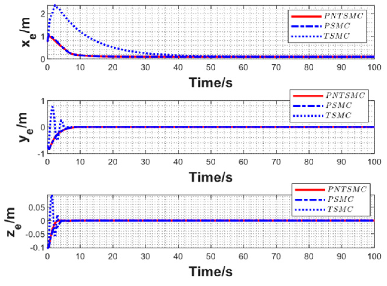
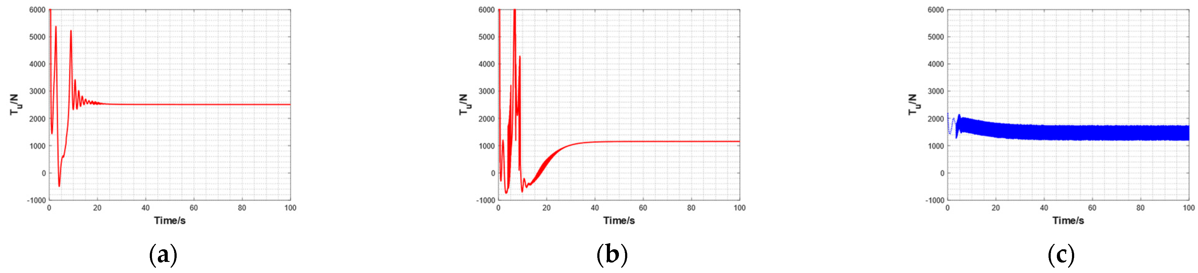
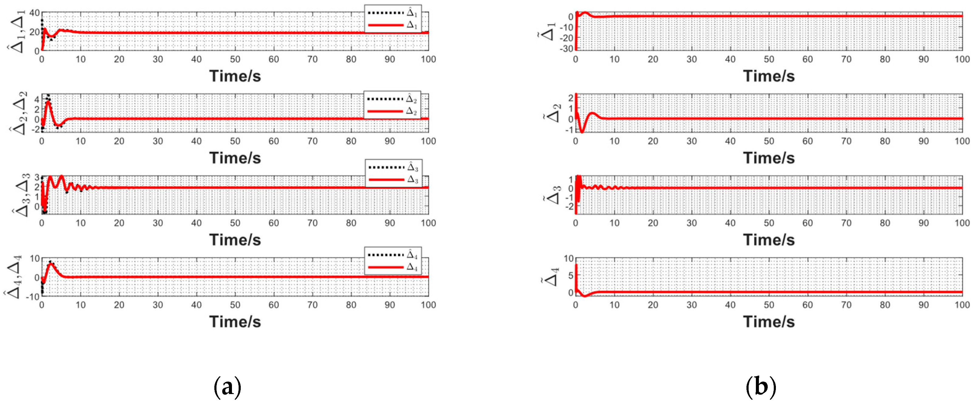
4. Numerical Simulation Example

To verify the effectiveness and robustness of the target tracking controller proposed in this paper, a numerical simulation has been performed on the “Qilin” underwater robot using MATLAB/Simulink^®. The “Qilin” underwater robot is a new prototype deep-sea work platform that can cruise in the deep sea and crawl on the bottom of the sea. The thruster layout and physical prototype of the robot are shown in Figure 6. Among them, $L_1$ = $L_2$ = 1 m; the thrust output of the four thrusters is −3000 to 3000 N. Thus, the limit of control moments and forces was −6000 to 6000 N(Nm) in simulation.

For this simulation, the control parameters are given in

Table 1. The control parameters.

Controller Function	Control Parameters
Non-singular terminal sliding mode function	$k_{\delta }=0.01$$,k_{\beta }=0.1$$,k_{\alpha }=0.01$$,k_{Z_e}=0.1$,
	$p_{\delta }=5$$,p_{\beta }=5$$,p_{\alpha }=5$$,p_{Z_e}=5$,
	$q_{\delta }=3$$,q_{\beta }=3$$,q_{\alpha }=3$$,q_{Z_e}=3$,
	$C_1=1$$,C_2=10$$,C_3=10$$,C_4=10$,
	${\kappa }_1=0.5$$,{\kappa }_2=0.5$$,{\kappa }_3=0.005$$,{\kappa }_4=0.001$.
Prescribed performance function	${\eta }_{10}=1$$,{\eta }_{1\infty }=0.2$$,{\eta }_{20}=1$$,{\eta }_{2\infty }=0.1$, ${\eta }_{30}=1$$,{\eta }_{3\infty }=0.1$$,{\eta }_{40}=1$$,{\eta }_{4\infty }=0.1$,
	$a_1=0.2$$,a_2=0.2$$,a_3=0.2$$,a_4=0.2$.
Error transformation function	$H_1=2$$,L_1=0.01$$,H_2=0.4$$,L_2=4$, $H_3=1.2$$,L_3=1.2$$,H_4=0.2$$,L_4=0.2$, $p_1=1$$,p_2=1$$,p_3=1$$,p_4=1$$,{\epsilon }_1=0.5$.
RBF neural network function	${\mathit{c}}_1=linspace\left(0,1.8,100\right)$$,{\mathit{c}}_2=linspace\left(-0.5,0.7,100\right)$$,{\mathit{c}}_3=linspace\left(-0.1,0.7,100\right)$$,{\mathit{c}}_4=linspace\left(-0.5,1.6,100\right)$,
	$b_1=0.5$$,b_2=1.5$$,b_3=0.4$$,b_4=1$,
	${\gamma }_1=0.7$$,{\gamma }_2=0.01$$,{\gamma }_3=0.8$$,{\gamma }_4=0.08$.

. The initial position and orientation of the underwater robot were $\left({\xi }_0,{\eta }_0,{\zeta }_0\right)=\left(1.25 \mathrm{m},1.25 \mathrm{m},100.1 \mathrm{m}\right)$ and $\left({\psi }_0,{\theta }_0\right)=\left(\frac{\pi }{2}rad,0rad\right)$; the initial velocity of the underwater robot was $\left(u_0,v_0,w_0\right)=\left(0 \mathrm{m}/\mathrm{s},0 \mathrm{m}/\mathrm{s},0 \mathrm{m}/\mathrm{s}\right)$. The initial position of the target was $\left({\xi }_{d0},{\eta }_{d0},{\zeta }_{d0}\right)=\left(2 \mathrm{m},2 \mathrm{m},100 \mathrm{m}\right)$, and the desired trajectory was generated by following typical timing laws:

$$\{\begin{array}{l}{\xi }_d=5\cos \left(\pi t/10\right)-3\hfill \\ {\eta }_d=5\sin \left(\pi t/10\right)+2\hfill \\ {\zeta }_d=-0.05t+100\hfill \end{array}$$

(45)

Equation (46) was introduced to simulate the bounded external disturbances.

$$\{\begin{array}{l}{\tau }_{ex1}=0.25sign\left(u\right)+0.5\sin \left(0.1t\right)\hfill \\ {\tau }_{ex2}=0.25sign\left(v\right)+0.5\sin \left(0.1t\right)\hfill \\ {\tau }_{ex3}=0.25sign\left(w\right)+0.5\sin \left(0.1t\right)\hfill \\ {\tau }_{ex4}=0.25sign\left(q\right)+0.5\sin \left(0.1t\right)\hfill \\ {\tau }_{ex5}=0.25sign\left(r\right)+0.5\sin \left(0.1t\right)\hfill \end{array}$$

(46)

The uncertainties of robot were as follows in the simulation:

$${\Delta }_i=5i+2.5\left|i\right|i+1.5i^3,i=u,v,w,q,r$$

(47)

Equation (46) and Equation (47) refer to [10].

To better verify the performance of the proposed controller, the proposed controller (PNTSMC) is compared with the nonsingular terminal sliding mode controller (TSMC) and the nonsingular terminal sliding mode controller with prescribed performance (PTSMC). The initial conditions for these controllers were the same.

Simulation results are illustrated in Figure 7, Figure 8, Figure 9, Figure 10 and Figure 11.

Figure 7 shows the trajectories of the underwater robot and the target. After cruising for a short distance, the trajectory of the underwater robot overlaps with that of the target. The results show that the three controllers can achieve accurate trajectory tracking in the presence of external disturbances and modeling uncertainties. In Figure 8, the tracking errors of PNTSMC and PTSMC could converge to zero with the prescribed performance and converge faster with less overshooting than those of TSMC. It can be observed in Figure 8 that the convergence process of PNTSMC is smoother than that of PTSMC. Figure 9 shows the posture errors. As $y_e$ and $z_e$ approach 0 m, $x_e$ approaches the safe distance $\tilde{\delta }=0.102$ m. It not only achieved convergence in the underactuated direction, but also avoided a collision, which shows the good performance of the tracking error and the success of the tracking guidance law. Figure 10 shows the control moments and forces generated by the three controllers. TSMC had the most dramatic chattering. Since the RBF neural network can approximate the unmodeled uncertainties, the gain of the sliding mode controller can be reduced to attenuate chattering. Simulation results show that chattering phenomenon of PNTSMC is weaker than that of PTSMC. From Figure 11, we can see that the RBF neural network effectively approximates the uncertainties of the underwater robot.

Remark 1.

If the chattering in Figure 10 cannot be tolerated by the thrusters, continuous saturation functions or hyperbolic tangent functions can be used to replace the sign functions to further attenuate chattering. However, this approach comes at the cost of losing control accuracy and reducing robustness.

In order to better understand the performance of different controllers, typical criteria such as steady-state error, convergence time and root mean square error are used for a quantitative comparison in

Table 2. Comparison of the performances of different controllers.

Quantitative Comparison	Control Scheme	${\mathit{\delta }}_{\left(\mathit{t}\right)}$	${\mathit{\beta }}_{\left(\mathit{t}\right)}$	${\mathit{\alpha }}_{\left(\mathit{t}\right)}$	${\mathit{Z}}_{\mathit{e}}{}_{\left(\mathit{t}\right)}$
Steady-state error	PNTSMC	0.0001 m	−1.6155 × 10−5°	7.4915 × 10−5°	−1.8646 × 10−5 m
	PTSMC	0.0001 m	7.2886 × 10−5°	0.0012°	−7.355 × 10−6 m
	TSMC	0.0030 m	1.848 × 10−4°	0.0019°	1.6467 × 10−6 m
Convergence Time	PNTSMC	10.59 s	4.351 s	4.639 s	2.625 s
	PTSMC	10.7 s	4.146 s	4.121 s	3.951 s
	TSMC	41.33 s	3.18 s	4.797 s	3.246 s
Root-mean-square error	PNTSMC	0.1870 m	0.3791°	3.1786°	0.0097 m
	PTSMC	0.1942 m	0.4598°	6.1865°	0.0104 m
	TSMC	0.6008 m	0.5070°	6.3648°	0.0109 m

. The steady-state error reflects the control accuracy and anti-disturbance ability of the system. The convergence time reflects the dynamic time of the system. In addition, root mean square error is reported to describe the controller’s control performance during the whole tracking process. Firstly, the results of the simulation for PNTSMC and TSMC are compared. It can be seen that PNTSMC has advantages over TSMC in steady-state error, which shows that PNTSMC can achieve more accurate tracking. As for the convergence time, the convergence times of tracking errors ${\delta }_{\left(t\right)}$, ${\alpha }_{\left(t\right)}$ and $Z_e{}_{\left(t\right)}$ were shortened by 30.74, 0.152 and 0.621 s, respectively—reduced by 74.4%, 3.2% and 19.1%. The convergence time of tracking error ${\beta }_{\left(t\right)}$ increased by 1.171 s, that is, 36.8%. In general, PNTSMC accelerated the convergence process. The root-mean-square errors of the tracking errors of the PNTSMC are all smaller, corresponding to ${\delta }_{\left(t\right)}$, ${\beta }_{\left(t\right)}$, ${\alpha }_{\left(t\right)}$ and $Z_e{}_{\left(t\right)}$, which were reduced by 0.4238, 0.1279, 3.1862 and 0.0012 m, respectively—70.5%, 25.2%, 50.1% and 11.0%. Secondly, for the comparison between PNTSMC and PTSMC, the gap between the two is very small by most criteria. The performance of PNTSMC was slightly better. In conclusion, we demonstrated the advantages of PNTSMC in rapid acquisition of stability and accurate trajectory tracking due to the prescribed performance technique.

According to the above results, the proposed controller can force an underwater robot to accurately track the desired target with prescribed steady-state and dynamic performances in the presence of modeling uncertainties and external disturbances. Overall, PNTSMC provides better dynamic performance, steady performance and chattering repression than the other two controllers.

5. Conclusions

To achieve good target tracking motion control performance in an environment with uncertainties and external disturbances, we designed a neural network non-singular terminal sliding mode controller for underactuated underwater robots with prescribed performances. By using non-singular terminal sliding mode and the RBF neural network, the controller achieves strong robustness against the modeling uncertainties and external disturbances. The prescribed performance technique ensures that the underwater robot has excellent target tracking control performance. Numerical simulations showed that the proposed controller has better dynamic performance, steady-state performance and chattering suppression, and can accomplish the target tracking task accurately and reliably in the presence of modeling uncertainties and external disturbances. The controller proposed in this paper is unique in its ability to achieve robustness against modeling uncertainties and the external disturbances, finite-time convergence, attenuating chattering and prescribed performances, simultaneously. It provides a new research topic for the target tracking control of underwater robots.

There are still some open problems to improve the target tracking control of underwater robots which are for future work:

• A hardware implementation of the proposed controller will be realized in a practical robot control system, and the possible concentration degree in the actual deployment would be discussed. Non-singular terminal sliding mode control and RBF neural networks have been used on a variety of platforms, and the prescribed performance technique only adds some logarithmic operations. In mainstream embedded computers, the computational load of the controller proposed in this paper is affordable. We will put this controller to the test in a computer with Intel^® Atom™ N455 as the core.
• When there is a large deviation in the tracking error, or when the underwater robot encounters a large disturbance, the prescribed performance technique may produce singular values. It is necessary to adaptively adjust the relevant parameters according to the real environment. At the same time, a finite-time performance function will be considered to improve the control performance.
• After comparing with PTSMC and TSMC, the method proposed in this paper should also be compared with other state-of-the-art positioning error and tracking error methods. This is one of the directions for further extending and improving the proposed controller.

References

1. Muthugala, M.A.V.J.; Samarakoon, S.M.B.P.; Elara, M.R. Toward energy-efficient online Complete Coverage Path Planning of a ship hull maintenance robot based on Glasius Bio-inspired Neural Network. Expert Syst. Appl. 2022, 187, 115940. [Google Scholar] [CrossRef]
2. Chi, X.; Zhan, Q. Design and Modelling of an Amphibious Spherical Robot Attached with Assistant Fins. Appl. Sci. 2021, 11, 3739. [Google Scholar] [CrossRef]
3. Song, C.; Cui, W. Review of Underwater Ship Hull Cleaning Technologies. J. Mar. Sci. Appl. 2020, 19, 415–429. [Google Scholar] [CrossRef]
4. Yu, C.; Xiang, X.; Wilson, P.A.; Zhang, Q. Guidance-Error-Based Robust Fuzzy Adaptive Control for Bottom Following of a Flight-Style AUV With Saturated Actuator Dynamics. IEEE Trans. Cybern. 2020, 50, 1887–1899. [Google Scholar] [CrossRef] [PubMed]
5. Tran, H.N.; Pham, T.N.N.; Choi, S.H. Robust depth control of a hybrid autonomous underwater vehicle with propeller torque’s effect and model uncertainty. Ocean Eng. 2021, 220, 108257. [Google Scholar] [CrossRef]
6. Cho, G.R.; Li, J.H.; Park, D.; Jung, J.H. Robust trajectory tracking of autonomous underwater vehicles using back-stepping control and time delay estimation. Ocean Eng. 2020, 201, 107131. [Google Scholar] [CrossRef]
7. Yan, Z.; Gong, P.; Zhang, W.; Wu, W. Model predictive control of autonomous underwater vehicles for trajectory tracking with external disturbances. Ocean Eng. 2020, 217, 107884. [Google Scholar] [CrossRef]
8. Gan, W.; Zhu, D.; Ji, D. QPSO-model predictive control-based approach to dynamic trajectory tracking control for unmanned underwater vehicles. Ocean Eng. 2018, 158, 208–220. [Google Scholar] [CrossRef]
9. Che, G.; Yu, Z. Neural-network estimators based fault-tolerant tracking control for AUV via ADP with rudders faults and ocean current disturbance. Neurocomputing 2020, 411, 442–454. [Google Scholar] [CrossRef]
10. Elhaki, O.; Shojaei, K. Neural network-based target tracking control of underactuated autonomous underwater vehicles with a prescribed performance. Ocean Eng. 2018, 167, 239–256. [Google Scholar] [CrossRef]
11. Guo, J.; Li, D.; He, B. Intelligent Collaborative Navigation and Control for AUV Tracking. IEEE Trans. Ind. Inform. 2021, 17, 1732–1741. [Google Scholar] [CrossRef]
12. Guo, Y.; Qin, H.; Xu, B.; Han, Y.; Fan, Q.Y.; Zhang, P. Composite learning adaptive sliding mode control for AUV target tracking. Neurocomputing 2019, 351, 180–186. [Google Scholar] [CrossRef]
13. Yan, Z.; Wang, M.; Xu, J. Global Adaptive Neural Network Control of Underactuated Autonomous Underwater Vehicles with Parametric Modeling Uncertainty. Asian J. Control. 2019, 21, 1342–1354. [Google Scholar] [CrossRef]
14. Miao, J.; Wang, S.; Zhao, Z.; Li, Y.; Tomovic, M.M. Spatial curvilinear path following control of underactuated AUV with multiple uncertainties. ISA Trans. 2017, 67, 107–130. [Google Scholar] [CrossRef] [PubMed]
15. Lamraoui, H.C.; Qidan, Z. Path following control of fully-actuated autonomous underwater vehicle in presence of fast-varying disturbances. Appl. Ocean Res. 2019, 86, 40–46. [Google Scholar] [CrossRef]
16. Zhang, Z.; Liu, B.; Wang, L. Autonomous underwater vehicle depth control based on an improved active disturbance rejection controller. Int. J. Adv. Robot. Syst. 2019, 16, 172988141989153. [Google Scholar] [CrossRef]
17. Ali, N.; Tawiah, I.; Zhang, W. Finite-time extended state observer based nonsingular fast terminal sliding mode control of autonomous underwater vehicles. Ocean Eng. 2020, 218, 108179. [Google Scholar] [CrossRef]
18. Elmokadem, T.; Zribi, M.; Youcef-Toumi, K. Terminal sliding mode control for the trajectory tracking of underactuated Autonomous Underwater Vehicles. Ocean. Eng. 2017, 129, 613–625. [Google Scholar] [CrossRef]
19. Patre, B.M.; Londhe, P.S.; Waghmare, L.M.; Mohan, S. Disturbance estimator based non-singular fast fuzzy terminal sliding mode control of an autonomous underwater vehicle. Ocean Eng. 2018, 159, 372–387. [Google Scholar] [CrossRef]
20. Wang, Z.; Liu, Y.; Guan, Z.; Zhang, Y. An Adaptive Sliding Mode Motion Control Method of Remote Operated Vehicle. IEEE Access 2021, 9, 22447–22454. [Google Scholar] [CrossRef]
21. Wang, Z.; Liu, Y.; Guan, Z.; Zhang, Y. Improved line-of-sight trajectory tracking control of under-actuated AUV subjects to ocean currents and input saturation. Ocean Eng. 2019, 174, 14–30. [Google Scholar] [CrossRef]
22. Yan, Z.; Wang, M.; Xu, J. Robust adaptive sliding mode control of underactuated autonomous underwater vehicles with uncertain dynamics. Ocean Eng. 2019, 173, 802–809. [Google Scholar] [CrossRef]
23. Mu, W.; Wang, Y.; Sun, H.; Liu, G. Double-Loop Sliding Mode Controller with An Ocean Current Observer for the Trajectory Tracking of ROV. J. Mar. Sci. Eng. 2021, 9, 1000. [Google Scholar] [CrossRef]
24. Zhang, Z.; Yan, W.; Li, H. Distributed Optimal Control for Linear Multiagent Systems on General Digraphs. IEEE Trans. Autom. Control. 2021, 66, 322–328. [Google Scholar] [CrossRef]
25. Zhang, Z.; Li, H.; Yan, W. Fully Distributed Control of Linear Systems with Optimal Cost on Directed Topologies. IEEE Trans. Circuits Systems. II Express Briefs 2021, 68, 336–340. [Google Scholar] [CrossRef]
26. Li, Z.; Liu, W.; Li, L.; Guo, L.; Zhang, W. Modeling and adaptive controlling of cable-drogue docking system for autonomous underwater vehicles. Int. J. Adapt. Control. Signal Processing 2021, 36, 354–372. [Google Scholar] [CrossRef]
27. Wu, H.; Song, S.; You, K.; Wu, C. Depth Control of Model-Free AUVs via Reinforcement Learning. IEEE Trans. Syst. Man Cybern.-Syst. 2017, 49, 2499–2510. [Google Scholar] [CrossRef] [Green Version]
28. Carlucho, I.; De Paula, M.; Wang, S.; Petillot, Y.; Acosta, G.G. Adaptive low-level control of autonomous underwater vehicles using deep reinforcement learning. Robot. Auton. Syst. 2018, 107, 71–86. [Google Scholar] [CrossRef] [Green Version]
29. Anderlini, E.; Parker, G.G.; Thomas, G. Docking Control of an Autonomous Underwater Vehicle Using Reinforcement Learning. Appl. Sci. 2019, 9, 3456. [Google Scholar] [CrossRef] [Green Version]
30. Sun, Y.; Zhang, C.; Zhang, G.; Xu, H.; Ran, X. Three-Dimensional Path Tracking Control of Autonomous Underwater Vehicle Based on Deep Reinforcement Learning. J. Mar. Sci. Eng. 2019, 7, 443. [Google Scholar] [CrossRef] [Green Version]
31. Cao, J.; Sun, Y.; Zhang, G.; Jiao, W.; Wang, X.; Liu, Z. Target tracking control of underactuated autonomous underwater vehicle based on adaptive nonsingular terminal sliding mode control. Int. J. Adv. Robot. Syst. 2020, 17, 172988142091994. [Google Scholar] [CrossRef]
32. Bechlioulis, C.P.; Rovithakis, G.A. Robust Adaptive Control of Feedback Linearizable MIMO Nonlinear Systems with Prescribed Performance. IEEE Trans. Autom. Control. 2008, 53, 2090–2099. [Google Scholar] [CrossRef]
33. Bechlioulis, C.P.; Karras, G.C.; Heshmati-Alamdari, S.; Kyriakopoulos, K.J. Trajectory Tracking with Prescribed Performance for Underactuated Underwater Vehicles Under Model Uncertainties and External Disturbances. IEEE Trans. Control. Syst. Technol. 2017, 25, 429–440. [Google Scholar] [CrossRef]
34. Liang, H.; Fu, Y.; Gao, J.; Cao, H. Finite-time velocity-observed based adaptive output-feedback trajectory tracking formation control for underactuated unmanned underwater vehicles with prescribed transient performance. Ocean Eng. 2021, 233, 109071. [Google Scholar] [CrossRef]
35. Shojaei, K.; Chatraei, A. Robust platoon control of underactuated autonomous underwater vehicles subjected to nonlinearities, uncertainties and range and angle constraints. Appl. Ocean Res. 2021, 110, 102594. [Google Scholar] [CrossRef]
36. Wang, Y.; Wang, H.; Li, M.; Wang, D.; Fu, M. Adaptive fuzzy controller design for dynamic positioning ship integrating prescribed performance. Ocean. Eng. 2021, 219, 107956. [Google Scholar] [CrossRef]
37. Li, J.; Du, J.; Hu, X. Robust adaptive prescribed performance control for dynamic positioning of ships under unknown disturbances and input constraints. Ocean Eng. 2020, 206, 107254. [Google Scholar] [CrossRef]
38. Fossen, T.I. Handbook of Marine Craft Hydrodynamics and Motion Control; John Wiley & Sons: Hoboken, NJ, USA, 2011. [Google Scholar]
39. Wang, W.; Huang, J.; Wen, C. Prescribed performance bound-based adaptive path-following control of uncertain nonholonomic mobile robots. Int. J. Adapt. Control Signal Processing 2017, 31, 805–822. [Google Scholar] [CrossRef]
40. Park, J.; Sandberg, I.W. Universal Approximation Using Radial-Basis-Function Networks. Neural Comput. 1991, 3, 246–257. [Google Scholar] [CrossRef]
Figure 1. Inertial reference coordinate system {I} and body reference coordinate system {B}.
Jmse 10 00252 g001
Figure 2. The range and bearing angles ( δ , β , α , Z e ) : (a) the horizontal projection of an underwater robot and tracking target; (b) the vertical plane projection of an underwater robot and tracking target.
Jmse 10 00252 g002
Figure 3. The prescribed performance and error transformation function: (a) a graphical illustration for the prescribed performance; (b) error transformation function f i .
Jmse 10 00252 g003
Figure 4. The block diagram of the proposed controller.
Jmse 10 00252 g004
Figure 5. RBF neural network structure.
Jmse 10 00252 g005
Figure 6. The underwater robot: (a) the thruster layout; (b) the physical prototype.
Jmse 10 00252 g006
Figure 7. The underwater robot trajectory and target trajectory: (a) η - ζ plane; (b) ξ - ζ plane; (c) ξ - η plane.
Jmse 10 00252 g007
Figure 8. The tracking errors with their performance bounds: (a) δ ( t ) ; (b) β ( t ) ; (c) α ( t ) ; (d) Z e ( t ) .
Jmse 10 00252 g008
Figure 9. The positional errors between the robot and the tracking target: x e , y e and z e .
Jmse 10 00252 g009
Figure 10. The control moments and forces T u , T q , T r and T w . (a) T u of PNTSMC; (b) T u of PTSMC; (c) T u of TSMC; (d) T q of PNTSMC; (e) T q of PTSMC; (f) T q of TSMC; (g) T r of PNTSMC; (h) T r of PTSMC; (i) T r of TSMC; (j) T w of PNTSMC; (k) T w of PTSMC; (l) T w of TSMC.
Jmse 10 00252 g010aJmse 10 00252 g010b
Figure 11. The total model uncertainty estimation: (a) the total uncertainties term Δ i ; the estimates of the total uncertainties term Δ ^ i ; (b) the errors of the above term Δ ˜ i .
Jmse 10 00252 g011