Multi-Objective Optimization of a Hydrogen Hub for the Decarbonization of a Port Industrial Area

Abstract

Green hydrogen is addressed as a promising solution to decarbonize industrial and mobility sectors. In this context, ports could play a key role not only as hydrogen users but also as suppliers for industrial plants with which they have strong commercial ties. The implementation of hydrogen technologies in ports has started to be addressed as a strategy for renewable energy transition but still requires a detailed evaluation of the involved costs, which cannot be separated from the correct design and operation of the plant. Hence, this study proposes the design and operation optimization of a hydrogen production and storage system in a typical Italian port. Multi-objective optimization is performed to determine the optimal levelized cost of hydrogen in environmental and techno-economic terms. A Polymer Electrolyte Membrane (PEM) electrolyzer powered by a grid-integrated photovoltaic (PV) plant, a compression station and two-pressure level storage systems are chosen to provide hydrogen to a hydrogen refueling station for a 20-car fleet and satisfy the demand of the hydrogen batch annealing in a steel plant. The results report that a 341 kW_P PV plant, 89 kW electrolyzer and 17 kg hydrogen storage could provide hydrogen at 7.80 €/kgH₂, potentially avoiding about 153 tCO_2,eq/year (120 tCO_2,eq/year only for the steel plant).

1. Introduction

It is widely accepted that the development of a green hydrogen economy could not only accelerate the renewable energy transition but also avoid the inequalities introduced by fossil energy sources [1]. The European Union (EU) has recently outlined some strategies to promote hydrogen production from Renewable Energy Sources (RES), and guidelines for the development of hydrogen systems are also available in Italy [2,3]. In addition to the clear advantages in terms of local emissions when hydrogen is used as fuel (e.g., in fuel cell vehicles), hydrogen is also one of the possible solutions to store energy produced from RES, e.g., solar and wind energy [4,5]. Compared to other electric storage systems such as lithium-ion or lead–acid batteries, hydrogen could be used for large seasonal energy storage. The stored hydrogen can then be reconverted into electricity via electrochemical devices (i.e., fuel cells) or directly used as fuel or chemical feedstock, e.g., in the “hard-to-abate” industry [6]. The International Energy Agency (IEA) [1] estimates that hydrogen could play a key role in the decarbonization of the iron and crude steel industries, which should decrease their CO₂ intensity by up to 2.5% annually in order to meet the restrictions by 2030. Sasiain et al. [7] calculated that the substitution of syngas derived from natural gas with green hydrogen could reduce CO₂ emissions by up to 88%, even if such an advantage was lost when the CO₂ intensity of the electricity network exceeded 125 gCO₂/kWh. Bhaskar et al. [8] estimated that coupling hydrogen direct reduction with Electric Arc Furnaces (EAF) could reduce emissions by up to 35% at the EU grid emission level of 295 gCO₂/kWh.

Nevertheless, although future investments aim to reduce the cost of green hydrogen, the cost of hydrogen production via electrolysis (≈10–20 $/kgH₂) is still not competitive with the cost of hydrogen produced via Steam Methane Reforming (SMR) or coal gasification processes (≈2 $/kgH₂) [9,10]. For example, Reddi et al. [11] estimated a hydrogen cost of 6–8 $/kgH₂ for a Hydrogen Refuelling Station (HRS) with 200 kgH₂/day of dispensing capacity. A recent analysis by Minutillo et al. [12] evaluated the Levelized Cost Of Hydrogen (LCOH) for hypothetical Italian refueling stations with on-site hydrogen production via water electrolysis. The LCOH resulted in a range between 9.29 €/kgH₂ and 12.48 €/kgH₂, depending on the size of the energy system and the electricity mix. Other studies addressed the preliminary design and optimization of green hydrogen energy systems with reference to both techno-economic and environmental aspects. For example, the studies proposed in [13,14] analyzed multi-energy systems and determined the photovoltaic (PV)–electrolyzer power ratio, which minimized the green hydrogen production cost. It should be noted that the optimal PV–electrolyzer power ratio depends on several effects, e.g., the cost of energy units, the energy available from RES, the hydrogen demand profiles. Castellanos et al. [13] identified an optimum power ratio between the PV and electrolyzer of 2.85, while in [14], the optimum power ratio was about equal to one.

Nevertheless, there seems to be a lack in the literature of studies addressing the optimization of hydrogen production and storage systems to fulfill the needs of a port industrial area, considering both industrial and mobility applications. In this framework, the present study investigates how green hydrogen produced from RES could be used to reduce fossil fuels consumption of internal transport and of an industrial plant in a typical Italian port. A multi-objective optimization model was developed to determine the optimal design and operation (D&O) of hydrogen production, storage and delivery systems located in a port industrial area. Two objective functions were defined to consider both techno-economic and environmental aspects. The optimization problem was formulated with a Mixed-Integer Linear Programming (MILP) approach, which allows us to limit the computational effort with respect to other mathematical approaches [15,16]. The proposed system encompasses a Polymer Electrolyte Membrane (PEM) electrolyzer, volumetric compressors and compressed hydrogen storage systems. A PV power plant integrated with the Italian electrical grid was included in the proposed energy system. The proposed analysis is based on cost data and a set of techno-economic assumptions that were collected from existing components. In the following, the proposed hydrogen system is described, and the main characteristics of the different components are presented. Afterwards, the D&O optimization model is outlined, and then the results are discussed.

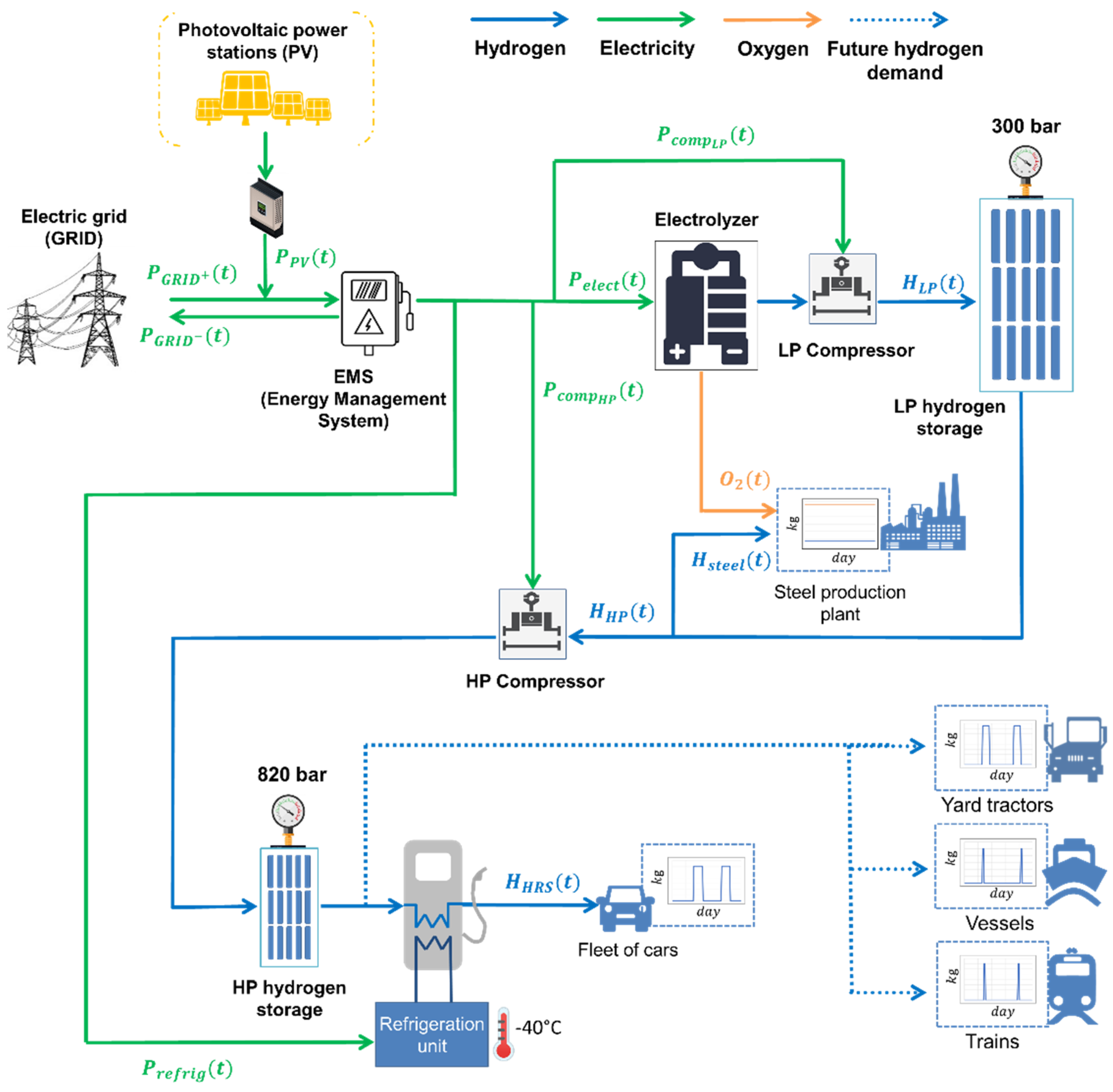
2. Proposed Plant Description

The industrial area of a typical port in the North-East of Italy was selected as a case study to assess the optimal D&O of a hydrogen production and delivery system. In particular, two hydrogen users were identified, namely an HRS to feed the car fleet of the port and a steel plant. The latter consists of a cold rolling plant for steel refining, which could use hydrogen for the annealing process in bell furnaces. For a preliminary analysis, it was assumed that a part of the hydrogen demand for the steel plant could be replaced with hydrogen produced from the proposed hydrogen production plant (~1000 kgH₂/month). As for the car fleet, 20 Fuel Cells Hybrid Vehicles (FCHV) were considered, and it has been assumed that each car covers 30 km/day. Such assumptions were made in accordance with data of the current car fleet in the port of Trieste, available in [17]. An average hydrogen consumption of 0.01 kgH₂/km and a 5-kg hydrogen tank capacity were assumed for each car [11,12]. A possible hydrogen refueling schedule was proposed with car refueling either at 7 a.m. or at 5 p.m. during weekdays. If, in the future, the HRS were to be dedicated to refueling more vehicles (including private ones), it would be necessary to evaluate a different refueling schedule such as the one proposed in [11].

Moreover, other possible users could be later included in the system, such as the public transport (e.g., buses, trains, ferries) and the internal transport in the port area (e.g., locomotives, forklifts, reach stackers, yard tractor, cranes, etc.) [18,19,20,21]. Figure 1 shows a simplified schematic of the analyzed hydrogen system. The green lines represent electricity flows, while hydrogen flows are reported in blue.

A PEM electrolyzer was chosen to produce high-purity hydrogen. The performance characteristics of the electrolyzer were evaluated on the basis of existing applications [1,10]. The electrolyzer is powered by electricity coming from the electric grid and/or from the PV plant, depending on the best strategy defined by the Energy Management System (EMS). It was assumed that excess electricity coming from the PV plant can be sold to the grid. The cost of the water flow feeding the electrolyzer was not considered in the calculation, since in Italy, it has a limited impact on the total production cost of hydrogen (<1%) [12]. Hydrogen produced at 30 bar is then compressed to 300 bar by a reciprocating compressor. This pressure level was chosen to find a compromise between the cost and volume occupied by the storage system. Compressed hydrogen could be used directly in the steel production plant or stored at 300 bar in the here called Low-Pressure (LP) storage system. The remaining part is further compressed to 820 bar and stored in a High-Pressure (HP) storage system for feeding the HRS. This pressure level allows the fast fueling of cars, without the use of compressors for transferring hydrogen to the vehicle tanks with a storage pressure of up to 700 bar. A refrigeration unit was considered at the dispenser to guarantee a hydrogen temperature during refueling of −40 °C [22]. The orange line in Figure 1 indicates the oxygen flow produced in the electrolysis process. While oxygen production was not considered in the optimization model, it could represent an additional revenue for the plant. The dashed blue lines indicate possible hydrogen demands for other vehicles that operate in the port and that could be included in the future.

3. Method

The set MILP optimization problem aims to find x*(t) and δ*(t) (i.e., the optimum values of the continuous, x, and binary, δ, decision variables associated with the design and operation of the energy system) that maximize or minimize the objective function Z (Equation (1)) subject to the constraint equations g(t) and inequalities h(t) (Equations (2) and (3)), which make up the model of the entire hydrogen system under consideration.

$$Z=f\left({\mathrm{x}}^{\ast }\left(t\right), {\mathsf{\delta }}^{\ast }\left(t\right)\right)$$

(1)

$$\mathrm{g}\left({\mathrm{x}}^{\ast }\left(t\right), {\mathsf{\delta }}^{\ast }\left(t\right)\right)=0$$

(2)

$$\mathrm{h}\left({\mathrm{x}}^{\ast }\left(t\right), {\mathsf{\delta }}^{\ast }\left(t\right)\right)\le 0$$

(3)

Section 3.1 introduces the g(t) and h(t) relationships in Equations (2) and (3), which describe the D&O of the energy conversion and storage units. Section 3.2 outlines the Z objective functions in Equation (1) and the adopted optimization approach.

3.1. Model for the Proposed Energy System

This section introduces the equations used to describe each energy conversion and storage unit embedded in the model as constraints of the optimization problem.

3.1.1. Photovoltaic Power Plant

The available solar energy was evaluated in agreement with the Italian standard UNI-10349 [23]. It was assumed that PV panels are installed on the buildings in the port area. The monocrystalline silicon panels are supposed to be arranged perfectly to the south with an inclination slope of 30°, albedo and Linke turbidity factors were set equal to 0.18 and 3, respectively. The PV efficiency (${\mathsf{\eta }}_{\mathrm{PV}}$) and the inverter efficiency (${\mathsf{\eta }}_{\mathrm{inverter}}$) were assumed constant at varying of the power load.

For each month, solar irradiance per hour ($P_{solar}\left(t\right)$) was calculated for the 15th day, assumed as the reference day for every single month. The PV peak power ($D_{PV}$) was constrained not to exceed the maximum available area for the PV plant (about 24.000 m²). Solar irradiance ($P_{solar}\left(t\right)$) was introduced as a fixed input variable of the system. The surface occupied by the PV plant ($Are{a}_{PV}$) and the power produced by the PV plant ($P_{PV}\left(t\right)$) were considered proportional to $D_{PV}$, neglecting the scale effect. An average value of about 8 kW_P/m² was considered for the PV panels ($coe{f}_{PV}$ in Equation (5)).

$$P_{PV}\left(t\right)={\mathsf{\eta }}_{\mathrm{PV}}·{\mathsf{\eta }}_{\mathrm{inverter}}·D_{PV}·P_{solar}\left(t\right)$$

(4)

$$D_{PV}=coe{f}_{PV}·Are{a}_{PV}$$

(5)

$$Are{a}_{PV}\le Are{a}_{PV,\max }$$

(6)

3.1.2. Electric Grid

The national electric grid is supposed to have an infinite power capacity for supplying/purchasing power to/from the considered energy system, with the hypothesis that costs of electricity (supplied and purchased) are constant during the year. In addition, voltage and frequency are assumed equal in both grid and hydrogen system networks.

3.1.3. Energy Management System

The energy management system sets out the operation of the energy system, managing the direction of the power flows. At each time step, the power balance in Equation (7) must be verified:

$$P_{PV}\left(t\right)+P_{GRID}^{+}\left(t\right)-P_{GRID}^{-}\left(t\right)=P_{elect}\left(t\right)+P_{com{p}_{LP}}\left(t\right)+P_{com{p}_{HP}}\left(t\right)+P_{refr}\left(t\right)$$

(7)

where $P_{GRID}^{+}\left(t\right)$ and $P_{GRID}^{-}\left(t\right)$ are the electric power purchased and sold from/to the grid at time t, respectively. $P_{elect}\left(t\right)$ is the input power of the electrolyzer, $P_{com{p}_{LP}}\left(t\right)$ is the input power of the low pressure (LP) compressor and $P_{compHP}\left(t\right)$ is the input power of the high pressure (HP) compressor.

3.1.4. Electrolyzer

The operation of the electrolyzer is described by the MILP Equations (8) and (9). The size of the electrolyzer ($D_{elect}$), i.e., the design power, is a decisional variable of the optimization problem.

$$H_{LP}\left(t\right)=k_{1_{elect}}·P_{elect}\left(t\right)·{\delta }_{elect}\left(t\right)$$

(8)

$$k_{2_{elect}}{D}_{elect}{\delta }_{elect}\left(t\right)\le P_{elect}\left(t\right)\le k_{3_{elect}} D_{elect}{\delta }_{elect}\left(t\right)$$

(9)

In Equation (8), $H_{LP}\left(t\right)$ indicates the hydrogen mass flow rate exiting the electrolyzer at time t, expressed as proportional to $P_{elect}\left(t\right)$ by a constant coefficient $k_{1_{elect}}$, which is determined according to the linearization of the performance curve of a typical electrolyzer at different power load [1,10]. ${\delta }_{elect}\left(t\right)$ is the binary variable that indicates the on/off status of the electrolyzer. In Equation (9), $k_{2_{elect}}$ and $k_{3_{elect}}$ set the load limits of the electrolyzer.

3.1.5. Compression Station

It is assumed that both LP and HP compressors are reciprocating compressors. In the following equations, the index j is used to indicate both LP and HP compressors. The electrical power absorbed by the j-th compressor ($P_{comp,j}$) is calculated as a function of the hydrogen mass flow rate ($H_j\left(t\right)$) entering the j-th compressor by means of the proportionality coefficient $k_{1_{comp,j}}$ (Equation (10)).

$$P_{comp,j}\left(t\right)=k_{1_{comp,j}}·H_j\left(t\right)$$

(10)

$k_{1_{comp,j}}$ in Equation (10) is calculated as reported in Equation (11), i.e., depending on: the mechanical efficiency of the compressor (${\eta }_{mech}$), the isentropic compression efficiency (${\eta }_{is}$), the electrical efficiency of the electric engine (${\eta }_{el}$) coupled with the compressor, and the ideal work of compression of an adiabatic isentropic compression ($L_{comp,id}$). The latter is determined as shown in Equation (12).

$$k_{1_{com{p}_j}}=\frac{L_{comp,id}}{{\eta }_{mech}· {\eta }_{is}·{\eta }_{el}}$$

(11)

$$L_{comp,id}=\frac{\gamma }{\gamma -1}R{T}_1\left[{\left(\frac{p_2}{p_1}\right)}^{\left(\frac{\gamma -1}{\gamma }\right)}-1 \right]$$

(12)

where $\gamma$ is the ratio between the specific heat at constant pressure and specific heat at constant volume, $R$ is the hydrogen gas constant, $T_1$ is the hydrogen inlet temperature (assumed in equilibrium with the surrounding environment), $p_1$ is the hydrogen inlet pressure ($p_{1,LP}$ for the LP compressor and $p_{2,LP}$ for the HP compressor) and $p_2$ is the hydrogen outlet pressure ($p_{2,LP}$ for the LP compressor and $p_{2,HP}$ for the HP compressor). $P_{comp,j}$ was constrained not to exceed the power load range (Equation (13)).

$$k_{2_{com{p}_j}}{D}_{com{p}_j}{\delta }_{comp,j}\left(t\right)\le P_{comp,j}\left(t\right)\le k_{3_{com{p}_j}}{D}_{com{p}_j}{\delta }_{comp,j}\left(t\right)$$

(13)

where $k_{2_{com{p}_j}}$ is the lower limit for compressor load, $k_{3com{p}_j}$ is the upper limit for compressor load, $D_{com{p}_j}$ is the compressor installed power, and ${\delta }_{com{p}_j}$ are the binary variables that define the on/off status of the compressors.

3.1.6. Hydrogen Storage Systems

Hydrogen is stored in compressed form at 300 bar (LP) or at 820 bar (HP). The hydrogen storage systems are described by Equations (14) to (17):

$$H_{S_{LP}}\left(t\right)=H_{S_{LP}}\left(t-1\right)+H_{LP}\left(t\right)-H_{steel}\left(t\right)-H_{HP}\left(t\right)$$

(14)

$$H_{S_{HP}}\left(t\right)=H_{S_{HP}}\left(t-1\right)+H_{HP}\left(t\right)-H_{HRS}\left(t\right)$$

(15)

$$k_{1_{s_j}}·D_{S_j}\le H_{S_j}\left(t\right)\le k_{2_{s_j}}·D_{S_j}$$

(16)

$$H_{S_j}\left(0\right)=H_{S_j}\left(t_{fin}\right)$$

(17)

where $H_{S_j}\left(t\right)$ is the hydrogen mass stored in the storage system, $H_{steel}\left(t\right)$ is the hydrogen mass flowrate flowing to the steel plant, $H_{HRS}\left(t\right)$ is the hydrogen mass flowrate directed to the HRS. $D_{S_j}$ is the storage system design capacity, and $k_{1_{s_j}}$ and $k_{2_{s_j}}$ are the lower and the upper limit for the storage system, respectively. It is set so that the hydrogen mass stored at the first-time step of the optimization is equal to the hydrogen mass stored at the last time step (Equation (17)).

3.1.7. Hydrogen Refueling Station

The HRS is assumed to be installed after the HP hydrogen storage to refuel the cars of the port fleet. For each vehicle of the fleet, the number of days ${\mathsf{\Delta }\mathrm{t}}_{ref}$ (days) after which hydrogen refueling is required is determined as shown in Equation (18):

$${\mathsf{\Delta }\mathrm{t}}_{ref}=\frac{{\alpha }_{tank}·M_{H2,tank}}{f_{km}·d_{day}}$$

(18)

where ${\alpha }_{tank}$ is the maximum hydrogen consumption before refueling, expressed as a percentage of the total mass capacity $M_{H2,tank}$ of the hydrogen tank. $f_{km}$ indicates the hydrogen consumption per km and $d_{day}$ is the distance covered in one day by a car.

The number of cars refueled per day is determined, assuming that refueling is possible only from Monday to Friday every week. Given the hydrogen consumption and the tank capacity of each car, the number of refuelings per day is two. As for the dispenser of the HRS, it is assumed that a single dispenser could supply about 50 kg/day, corresponding to the refueling of ten cars per day. During refilling, each dispenser has a hydrogen mass flow rate (${\dot{m}}_{d,H2}$) evaluated as shown in Equation (19) and constrained not to exceed the maximum hydrogen flowrate during a refilling $\left({\dot{m}}_{d,H2,max}\right)$ (Equation (20)).

$${\dot{m}}_{d,H2}=\frac{{\alpha }_{tank}·M_{H2,tank}}{t_{ref}}$$

(19)

$${\dot{m}}_{d,H2}\le {\dot{m}}_{d,H2,max}$$

(20)

where $t_{ref}$ is the refueling time. ${\dot{m}}_{d,H2,max}$ is defined in accordance with the refueling protocol SAE-J2601 [22]. The latter also requires that a refrigeration unit is encompassed in the system in order to avoid possible safety issues related to the increase of hydrogen temperature during refueling.

The power required for the refrigeration of hydrogen ($P_{refr}$) is determined as in Equation (21):

$$P_{refr}\left(t\right)=\frac{H_j\left(t\right)·\left(h_{storage}-h_{dispenser}\right)}{COP}$$

(21)

where $h_{storage}$ is the hydrogen enthalpy at HP storage, and $h_{dispenser}$ is the hydrogen enthalpy at the dispenser, both determined according to CoolProp libraries [24,25] as a function of hydrogen pressure and temperature. $COP$ indicates the coefficient of performance of the refrigeration unit.

3.2. Objective Functions

Multi-objective optimization was performed using the MILP solver Gurobi Optimizer to determine the best D&O of the proposed hydrogen system [26]. A blended objectives method was adopted, considering a linear combination of the objective functions, each with a fixed weight [22].

In this work, two objective functions were specified, namely LCOH ($f_1$ in Equation (22)) and $C{O}_{2,eq}$ emissions ($f_2$ in Equation (23)). To obtain the blend of the two objective functions, the emissions of $C{O}_{2,eq}$ were introduced as a cost in the $f_{1,2}$ (Equation (24)) by imposing a cost for tons of $C{O}_{2,eq}$ emitted, i.e., a carbon tax, as the weight $w_2$ of the function $f_2$. This is a strategy adopted by several authors in the energy field to evaluate the environmental impacts of energy systems, for example, by [27]. It should be noticed that in Italy no carbon tax is set yet, hence the value of $w_2$ was set to 50 €/t_CO2,eq according to the average values for Europe and the 2030 projections for effective carbon rates in OECD countries [28,29]. The weight of $f_1$ ($w_1$) is set equal to 1.

A 1% deviation from the optimal value of the $f_{1,2}$ function is permitted.

$$f_1=minimize \left(Levelized Cost Of Hydrogen\right)$$

(22)

$$f_2=minimize\left(C{O}_{2,eq} emissions\right)$$

(23)

$$f_{1,2}=w_1\ast f_1+w_2\ast f_2$$

(24)

In this case, the $C{O}_{2,eq}$ emissions depend only on the carbon intensity of the electrical grid and are hence calculated by multiplying the grid carbon factor $C{O}_{2, GRID}$ by the power absorbed from the grid $P_{GRID}^{+}\left(t\right)$ (Equation (25)).

$$C{O}_{2,eq}=C{O}_{2, GRID}{\displaystyle \sum }\left(P_{GRID}^{+}\left(t\right)\right)$$

(25)

The LCOH is calculated as shown in Equation (26), where $C_{inv,a_j}$ is the annualized capital cost of the j-th energy conversion or storage unit, $C_{rep,a_j}$ the replacement cost, $C_{O\&M_j}$ the yearly cost for operation and maintenance of each unit, $c_{GRID}^{+}$ and $c_{GRID}^{-}$ are the cost of electricity purchased and sold from/to the grid, respectively.

$$\mathrm{LCOH}=\frac{{\displaystyle \sum }{D}_j\left(C_{inv,a_j}+C_{rep,a_j}+C_{O\&M_j}\right)+c_{GRID}^{+}{\displaystyle \sum }{P}_{GRID}^{+}\left(t\right)-c_{GRID}^{-}{\displaystyle \sum }{P}_{GRID}^{-}\left(t\right)}{H_{2,demand}}$$

(26)

Equations (27) and (29) report how annualized investment and replacemet costs are calculated. $i$ is the nominal interest rate, $n$ is the assumed plant lifetime, $L{T}_j$ is the assumed lifetime of the j-th unit, $C_{in{v}_j}$ is the investment cost for the j-th unit. It is assumed that, at the end-of-life, the components are replaced with the same capital costs (Equation (27)). $C_{O\&M_j}$ are calculated as dependent on the $C_{inv,a_j}$ by the proportionality coefficient $c_{O\&M_j}$ (Equation (29)).

$$C_{inv,a_j}=\frac{i{\left(1+i\right)}^n}{i{\left(1+i\right)}^n-1}\ast C_{in{v}_j}$$

(27)

$$C_{rep,a_j}=\frac{i{\left(1+i\right)}^n}{i{\left(1+i\right)}^n-1}\ast \frac{C_{in{v}_j}}{{\left(1+i\right)}^{L{T}_j} }$$

(28)

$$C_{O\&M_j}=c_{O\&M_j}\ast C_{in{v}_j}$$

(29)

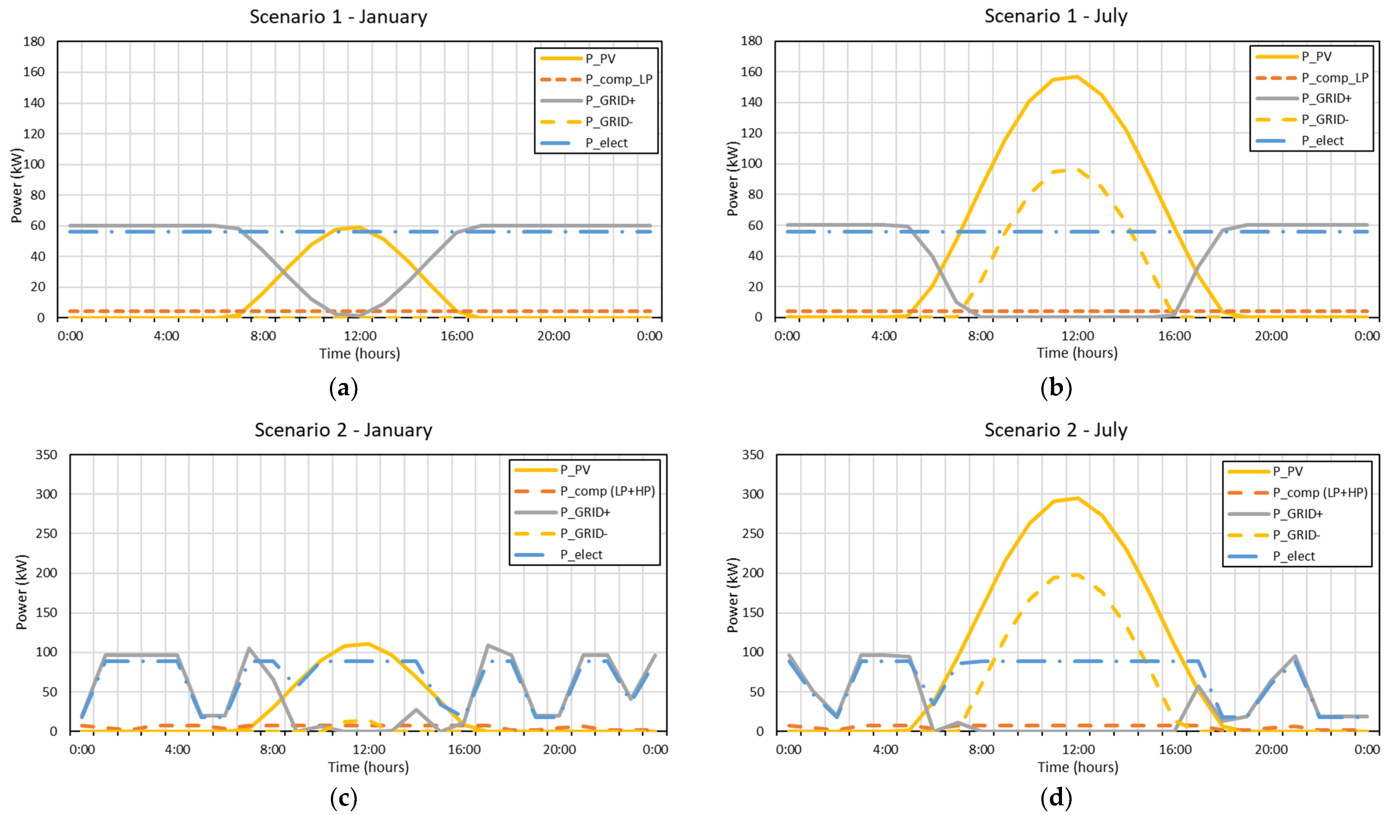
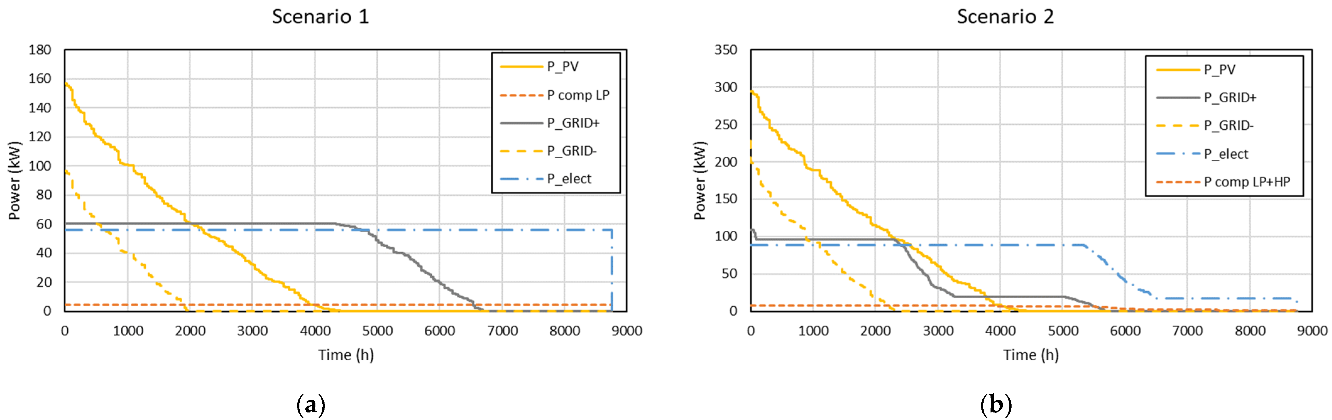
4. Results and Discussion

This section presents the parameters and assumptions adopted for the multi-objective optimization, and the main results of the optimization, which are discussed in the last part of Section 4.2.

4.1. Parameters and Assumptions of the Optimization Model

Table 1. Parameters and assumptions considered for the D&O optimization model. Data extracted and elaborated from [1,10,11,12,22,28,29,30,31,32].

Model Parameters	Value	Unit	Parameter Description	References
PV
$Are{a}_{PV,max}$	24,000	m2	Max available surface for PV installation	Assumed
$coe{f}_{PV}$	8	kWP/m2	PV power per square meter	[30]
${\eta }_{PV}$	0.2	-	Average efficiency	[30]
${\eta }_{inverter}$	0.95	-	Inverter average efficiency	[30]
$c_{PV}$	1000	€/kWP	Investment cost	[30]
$c_{O\&M_{PV}}$	1.58	%	Operation and maintenance cost	[30]
$L{T}_{PV}$	15	years	PV lifetime	[30]
Electrolyzer
$k_{1_{elect}}$	0.019	kgH2/kW	Coefficient of proportionality	[1,10]
$k_{2_{elect}}$	0.2	-	Lower power load limit	[1,10]
$k_{3_{elect}}$	1	-	Upper power load limit	[1,10]
$c_{elect}$	2000	€/kW	Investment cost	[1,10]
$c_{O\&M_{elect}}$	2.00	%	Operation and maintenance cost	[11,12]
$L{T}_{elect}$	15	years	Electrolyzer lifetime	[1,10]
Compression station
$k_{2_{com{p}_{LP}}}$	0.2	-	Lower load limit of LP compressor	Assumed
$k_{3_{com{p}_{LP}}}$	1	-	Upper load limit of LP compressor	Assumed
$k_{2_{com{p}_{HP}}}$	0.2	-	Lower load limit of HP compressor	Assumed
$k_{3_{com{p}_{HP}}}$	1	-	Upper load limit of HP compressor	Assumed
$\gamma$	1.4	-	H2 specific heat ratio	Assumed
$R$	4.12		H2 gas constant	Assumed
$T_1$	25	°C	H2 inlet temperature of LP/HP compressors	Assumed
$p_{1,LP}$	300	bar	H2 inlet pressure of LP compressor	Assumed
$p_{1,HP}$	820	bar	H2 inlet pressure of HP compressor	[11,12]
$p_{2,LP}$	30	bar	H2 outlet pressure of LP compressor	[1,10]
$p_{2,HP}$	300	bar	H2 outlet pressure of LP compressor	Assumed
${\eta }_{mech}$	98	%	Mechanical efficiency	[11,12]
${\eta }_{is}$	80	%	Isentropic efficiency	[11,12]
${\eta }_{el}$	96	%	Electric efficiency of the engine	[11,12]
$c_{com{p}_{LP}}$	7000	€/kW	Investment cost of LP compressor	[11,12]
$c_{com{p}_{HP}}$	7000	€/kW	Investment cost of HP compressor	[11,12]
$c_{O\&M_{com{p}_{LP}}}$	8.00	%	Operation and maintenance cost of LP compressor	[11,12]
$c_{O\&M_{comp\_HP}}$	8.00	%	Operation and maintenance cost of HP compressor	[11,12]
$L{T}_{com{p}_{LP}}$	20	years	LP compressor lifetime	[11,12]
$L{T}_{com{p}_{HP}}$	20	years	HP compressor lifetime	[11,12]
H2 storage systems
$c_{S_{LP}}$	1500	€/kgH2	Investment cost of the low-pressure H2 storage	[1,10]
$c_{S_{HP}}$	1500	€/kgH2	Investment cost of the high-pressure H2 storage	[1,10]
$c_{O\&M_{S_{LP}}}$	0	%	Operation and maintenance cost of the LP H2 storage	[11,12]
$c_{O\&M_{S_{HP}}}$	0	%	Operation and maintenance cost of the HP H2 storage	[11,12]
$L{T}_{S_{LP}}$	25	years	LP H2 storage lifetime	[1,10]
$L{T}_{S_{HP}}$	25	years	HP H2 storage lifetime	[1,10]
H2 refueling station
$M_{H2,tank}$	5	kg	Total mass capacity of the onboard H2 tank	[11,12]
$d_{day}$	30	km/day	Distance covered in one day per car	Assumed
$f_{km}$	0.01	kgH2/km	H2 consumption per km	Assumed
${\alpha }_{tank}$	80	%	Max H2 consumption before refueling	Assumed
$t_{ref}$	5	min	Refueling time	[11,12]
${\dot{m}}_{H2,max}$	60	gH2/s	H2 mass flow rate	[22]
$COP$	1	-	Coefficient of performance	[12]
$c_{dispenser}$	270,000	€/unit	Investment cost of the dispenser	[31]
$c_{refrig}$	5374	€/kW	Investment cost of the cooling system	[11,12]
$c_{O\&M_{dispenser}}$	3.00	%	Operation and maintenance cost of the dispenser	[11,12]
$c_{O\&M_{refrig}}$	3.00	%	Operation and maintenance cost of the cooling system	[11,12]
$L{T}_{dispenser}$	10	years	Dispenser lifetime	[11,12]
$L{T}_{refrig}$	15	years	Cooling system lifetime	[11,12]
Others
$c_{GRID}^{+}$	0.12	€	Cost of the electricity purchased from the grid	[32]
$c_{GRID}^{-}$	0.05	€	Cost of the electricity sold to the grid	[32]
$w_2$	50	€/tCO2,eq	Carbon tax	[28,29]
$n$	25	years	Plant lifetime	Assumed
$i$	5	%	Nominal interest rate	Assumed

shows the parameters and assumptions adopted in the model for multi-objective optimization. The evaluation of the techno-economic performances for the energy storage and conversion units is a key result of the study, as it is representative of the current Italian market scenario.

4.2. Main Results of the D&O Optimization

The multi-objective optimization was performed for two energy system scenarios: the first one (Scenario 1) considers only the hydrogen demand of the steel production plant $\left(H_{steel}\right)$, the second one (Scenario 2) considers the hydrogen demand of both the steel production plant and the HRS $\left(H_{steel}+H_{HRS}\right)$. The results of the multi-objective optimization are shown in

Table 2. Results of the D&O optimization for the two energy system scenarios.

Scenario	$D_{PV}$ $\left(k{W}_P\right)$	$D_{elect}$ $\left(kW\right)$	$D_{com{p}_{LP}}$ $\left(kW\right)$	$D_{com{p}_{HP}}$ $\left(kW\right)$	$D_{S_{LP}}$ $\left(kg\right)$	$D_{S_{HP}}$ $\left(kg\right)$	$LCOH$ $\left(\mathit{€}/kg\right)$	$LCO{H}^{\ast }$ $\left(\mathit{€}/kg\right)$	$C{O}_{2,eq}$ $\left(kg/k{g}_{H_2}\right)$
1	182	56	4.29	-	0	-	7.03	7.52	9.75
2	341	89	6.82	0.73	10	7	7.41	7.80	7.70

and

Table 3. Results of the D&O optimization for the two energy system scenarios, with a fixed value of the PV power installed.

Scenario	$D_{PV}$ $\left(k{W}_P\right)$	$D_{elect}$ $\left(kW\right)$	$D_{com{p}_{LP}}$ $\left(kW\right)$	$D_{com{p}_{HP}}$ $\left(kW\right)$	$D_{S_{LP}}$ $\left(kg\right)$	$D_{S_{HP}}$ $\left(kg\right)$	$LCOH$ $\left(\mathit{€}/kg\right)$	$LCO{H}^{\ast }$ $\left(\mathit{€}/kg\right)$	$C{O}_{2,eq}$ $\left(kg/k{g}_{H_2}\right)$
1	500	56	4.29	-	0	-	7.61	8.04	8.58
1	1000	75	5.73	-	9	-	8.92	9.22	6.07
1	2000	89	6.81	-	23	-	11.55	11.75	4.04
1	3000	100	7.69	-	23	-	14.08	14.21	2.58
2	500	93	7.13	0.85	11	6	7.66	8.00	6.74
2	1000	103	7.88	0.85	16	6	8.65	8.90	5.00
2	2000	121	9.24	0.85	25	6	10.81	10.95	2.75
2	3000	119	9.18	0.85	26	6	12.94	13.07	2.54

. The corresponding $f_1$ values (Equation (22)) are reported in the “LCOH” columns. The optimal values of $f_{1,2}$ (Equation (24)) are reported in the “LCOH*” column. The results in Table 2 report the design values of the energy conversion and storage units, the LCOH (considering/not considering the cost of related $C{O}_{2,eq}$ emissions) and the $C{O}_{2,eq}$ emissions per kg of the produced hydrogen. This last parameter strongly depends on the Italian grid energy mix and on the amount of power taken from the grid. In fact, the high values of $C{O}_{2,eq}$ obtained in the Scenario 1 and Scenario 2 optimizations are due to the large amount of energy purchased from the grid (340 MWh and 315 MWh, respectively, for Scenario 1 and 2). In Scenario 1, the electrolyzer results are to be designed for operating at the rated power over the year, providing hydrogen directly to the steel plant (constant hydrogen demand), without the need for a hydrogen storage system. In this case, the PV plant has power production during winter in line with the power demand profile of the hydrogen production plant. During the summer season, the exceeding power generated by the PV plant is sold to the grid, while during the winter season, the PV power is not sufficient to power the electrolyzer and electricity is purchased from the grid. As a consequence, the produced hydrogen results have $C{O}_{2,eq}$ emissions comparable with the ones of grey hydrogen produced via SMR (about 10 kgCO_2,eq/kg_H2) [1]. Differently, lower $C{O}_{2,eq}$ emissions can be achieved in Scenario 2, thanks to the increased installed power. Indeed, the PV-Electrolyzer power ratio is 3.83 for Scenario 2, while in Scenario 1, it is equal to 3.25. For Scenario 2, hydrogen storage systems are required for both LP and HP hydrogen storage systems. The HP storage system is required to provide hydrogen for the cars without increasing the electrolyzer rated power. The LP storage system allows the storage of the surplus hydrogen produced during daylight hours.

Table 3 reports the results of D&O optimization with a fixed value for $D_{PV}$, i.e., a set design for the PV plant. Four sizes of PV were considered: 500 kW_P, 1000 kW_P, 2000 kW_P and 3000 kW_P. As reported in Table 3, the increase of PV rated power causes a reduction of $C{O}_{2,eq}$ emissions and an increase in LCOH* with respect to the result reported in Table 2. For both Scenario 1 and Scenario 2, the electrolyzer rated power tends not to increase with the increase in PV installed. In fact, the PV–Electrolyzer power ratio increases with the increase of the PV rated power (from 8.9 to 30 for Scenario 1, from 5.3 to 25 for Scenario 2), while the electrolyzer utilization factor, i.e., the ratio between the electrolyzer energy demand over the year and its rated power, tends to decrease with an increase of the LP storage system capacity. It should be noted that by increasing the penetration of RES in the grid energy mix, the carbon impact of hydrogen production may be lower. For example, the $C{O}_{2,eq}$ emissions could change in the future by modifying the contract with the distributor, i.e., purchasing “cleaner” power from the grid. Another way to approach the zero-emissions hydrogen production is to increase both the power installed for the PV and the electrolyzer and the capacity of the hydrogen storage. In this way, it could be possible to decrease the amount of electricity purchased from the grid, even though this may not be convenient in energy and economic terms. In fact, electrolyzers, compressors and storage systems would be oversized, resulting in lower utilization factors and higher costs.

Figure 2 shows the results of D&O optimization for Scenario 1 (Figure 2a,b) and Scenario 2 (Figure 2c,d). Power flows at the EMS level are shown for both scenarios during a typical winter day (15th January) and a typical summer day (15th July), while duration curves for the optimal plant operation over the whole year are reported in Figure 3.

From Figure 2, it emerges that for both Scenario 1 and Scenario 2, the power produced by the PV power plant (solid yellow curves) in the two typical days is considerably different due to the relevant variation of the solar irradiance during the year. This also reflects on the different profiles of the power sold to the grid (dashed yellow curves), which is practically null during the winter season. On the contrary, the power purchased from the grid (solid grey curves) and the power required by the electrolyzer (dashed blue curves) has similar profiles in the summer and winter days. Indeed, electrolyzer is designed to be optimally coupled with PV power produced in the winter season. Looking at Figure 3, it can be noticed that the utilization factor of the electrolyzer is 8580 hours for Scenario 1 (Figure 3a) and 6315 hours for Scenario 2 (Figure 3b). From Figure 3, it can also be retrieved that the amount of energy purchased from the grid (area under the grey, solid lines in Figure 3) is higher for Scenario 1 than for Scenario 2, given the lower availability of energy from the PV plant in the first case (182 kW_p installed power) with respect to the second case (341 kW_p installed power).

By considering the hydrogen demand for the steel production plant to be fulfilled by grey hydrogen (i.e., produced via SMR), it the amount of avoided $C{O}_{2,eq}$ emissions is estimated. According to the current European grey hydrogen production technologies, the carbon impact per kg of grey hydrogen (normally used as industrial feedstock) is about 10 kg of $C{O}_{2,eq}$ [1]. As for the car fleet, assuming a $C{O}_{2,eq}$ emission factor of 149 $C{O}_{2,eq}/km$ (calculated as the average emission factor of Euro 2, 3, 4, 5 and 6 vehicles classes), it results in an overall amount of $C{O}_{2,eq}$ emissions of the current car fleet of about 33 $tonC{O}_{2,eq}/year$, which could be avoided by substituting diesel-fueled vehicles with FCHV [33,34]. With the set optimization parameters, the reduction of $C{O}_{2,eq}$ emissions of Scenario 1 could be relevant with the increase in the PV rated power, i.e., by increasing the LCOH. For example, with a 1 MW_P PV plant, about 50 $tonC{O}_{2,eq}/year$ emissions could be avoided. Similar considerations can be made for Scenario 2, where a 1 MW_P PV plant would allow 77 tons of $C{O}_{2,eq}$ emissions reduction. If hydrogen demand were to be met with 100% green hydrogen, about 120 tons of $C{O}_{2,eq}$ emissions could be saved each year for the only steel plant (Scenario 1).

In general, if low carbon impact needs to be achieved, it should be met a compromise with the production cost. The latter could be reduced either by increasing the production of hydrogen during the time period with high availability of RES or by modifying the purchasing contract with the grid (e.g., imposing a higher RES share). The potential decarbonization of industrial and mobility sectors depends on the cost that users are willing to accept for reaching an environmental target.

The results could be different if a power demand of the port industrial area was considered, as in this case, part of the PV power could directly cover part of the electricity demand. However, the electricity self-consumption may result in greater decarbonization of the industrial plant and an increase in revenues for the power produced by the PV plant. In addition, the oxygen recovery could also reduce the cost of green hydrogen, providing new revenue for the hydrogen system. Assuming a price of gaseous oxygen varying between 1 and 7 €/kg O₂ [35], the oxygen recovery could provide an additional profit in a range between 120 and 820 k€/year.

5. Conclusions

This study proposes a multi-objective optimization model to define the optimal D&O of a hydrogen production system in techno-economic and environmental terms. The LCOH is evaluated for two proposed scenarios in a typical Italian port area, considering the hydrogen demand of a steel plant and the combination of both the steel plant and HRS hydrogen demand. Taking into account the cost of the related carbon impact in hydrogen production, the LCOH* results are approximately 7.52 $€/k{g}_{H_2}$ for Scenario 1, and 7.80 $€/k{g}_{H_2}$ for Scenario 2. The hydrogen production cost could decrease with the reduction of hydrogen technologies (electrolyzer, compressors and storage systems) costs or with an increase in the price of electricity produced from PV and sold to the grid. The potential decrease of carbon impact depends on the PV and electrolyzer rated powers and the capacity of hydrogen storage systems. As for the proposed energy system configurations, the reduction of carbon impact is between 3 and 89 tons of $C{O}_{2,eq}$ emissions avoided per year for Scenario 1, and between 35 and 114 tons of $C{O}_{2,eq}$ emissions avoided per year for Scenario 2.

A higher carbon tax could be considered for further analysis. It should be noted that, taking into account the cost for $C{O}_{2,eq}$ emissions of the existing applications, the revenues provided from the avoided emissions may be relevant and could entail increased power for the PV plant or a reduced utilization factor of the electrolyzer. However, these applications are now excluded from this type of taxation. Environmental bonuses could encourage the substitution of diesel cars with an FCHV or the substitution of grey hydrogen with green hydrogen in steel plants. In addition, further analysis could consider the recovery of oxygen produced by the electrolyzer. In fact, the recovered oxygen could contribute to the decarbonization of steel plants when replacing the oxygen currently used and commonly produced by air separation plants.

The proposed analysis has general validity, and it is useful not only for the design and for the operation of the specific hydrogen system considered in this study but also for other industrial areas.

Further analyses could extend the use of hydrogen to other vehicles (e.g., cargo handling equipment and ships) or industrial users (e.g., chemical plants) in port areas. The uncertainty analysis on whether and how the optimization results are affected by stochastic input parameters, such as the cost of electricity and of equipment, could also be investigated in future insights.

References

1. International Energy Agency (IEA). The Future of Hydrogen; International Energy Agency: Paris, France, 2019. [Google Scholar]
2. European Commission. A Hydrogen Strategy for a Climate-Neutral Europe; European Commission: Brussels, Belgium, 2020. [Google Scholar]
3. Italian Ministry for Economic Development National. Strategy for Hydrogen, Preliminary Guidelines; Italian Ministry for Economic Development National: Rome, Italy, 2020. [Google Scholar]
4. Gutiérrez-Martín, F.; Amodio, L.; Pagano, M. Hydrogen production by water electrolysis and off-grid solar PV. Int. J. Hydrogen Energy 2021, 46, 29038–29048. [Google Scholar] [CrossRef]
5. Kotowicz, J.; Jurczyk, M.; Węcel, D. The possibilities of cooperation between a hydrogen generator and a wind farm. Int. J. Hydrogen Energy 2021, 46, 7047–7059. [Google Scholar] [CrossRef]
6. Kovač, A.; Paranos, M.; Marciuš, D. Hydrogen in energy transition: A review. Int. J. Hydrogen Energy 2021, 46, 10016–10035. [Google Scholar] [CrossRef]
7. Sasiain, A.; Rechberger, K.; Spanlang, A.; Kofler, I.; Wolfmeir, H.; Harris, C.; Bürgler, T. Green Hydrogen as Decarbonization Element for the Steel Industry. BHM Berg- und Hüttenmännische Monatshefte 2020, 165, 232–236. [Google Scholar] [CrossRef]
8. Bhaskar, A.; Assadi, M.; Somehsaraei, H.N. Decarbonization of the Iron and Steel Industry with Direct Reduction of Iron Ore with Green Hydrogen. Energies 2020, 13, 758. [Google Scholar] [CrossRef] [Green Version]
9. Calise, F.; D’Accadia, M.D.; Santarelli, M.; Lanzini, A.; Ferrero, D. Solar Hydrogen Production; Accademic Press: Cambridge, MA, USA, 2019. [Google Scholar]
10. IRENA. Green Hydrogen Cost Reduction: Scaling up Electrolysers to Meet the 1.5⁰C Climate Goal; International Renewable Energy Agency: Abu Dhabi, United Arab Emirates, 2020. [Google Scholar]
11. Reddi, K.; Elgowainy, A.; Rustagi, N.; Gupta, E. Impact of hydrogen refueling configurations and market parameters on the refueling cost of hydrogen. Int. J. Hydrogen Energy 2017, 42, 21855–21865. [Google Scholar] [CrossRef]
12. Minutillo, M.; Perna, A.; Forcina, A.; Di Micco, S.; Jannelli, E. Analyzing the levelized cost of hydrogen in refueling stations with on-site hydrogen production via water electrolysis in the Italian scenario. Int. J. Hydrogen Energy 2021, 46, 13667–13677. [Google Scholar] [CrossRef]
13. Castellanos, J.G.; Walker, M.; Poggio, D.; Pourkashanian, M.; Nimmo, W. Modelling an off-grid integrated renewable energy system for rural electrification in India using photovoltaics and anaerobic digestion. Renew. Energy 2015, 74, 390–398. [Google Scholar] [CrossRef] [Green Version]
14. Loong, Y.T.; Dahari, M.; Yap, H.J.; Chong, H.Y. Development of a system configuration for a solar powered hydrogen facility using fuzzy logic control. J. Zhejiang Univ. Sci. A 2013, 14, 822–834. [Google Scholar] [CrossRef] [Green Version]
15. Ito, K.; Yokoyama, R.; Akagi, S.; Yamaguchi, T.; Matsumoto, Y. Optimal Operational Planning of a Gas Turbine Combined Heat and Power Plant Based on the Mixed-Integer Programming. IFAC Proc. Vol. 1988, 21, 371–377. [Google Scholar] [CrossRef]
16. Rech, S. Smart Energy Systems: Guidelines for Modelling and Optimizing a Fleet of Units of Different Configurations. Energies 2019, 12, 1320. [Google Scholar] [CrossRef] [Green Version]
17. Sustainable Ports in the Adriatic-Ionian Region (SUPAIR) Website. Action Plan for a Sustainable and Low carbon Port of Trieste. Available online: https://supair.adrioninterreg.eu/library/7-action-plans-for-sustainable-and-low-carbon-ports (accessed on 24 January 2022).
18. van Biert, L.; Godjevac, M.; Visser, K.; Aravind, P.V. A review of fuel cell systems for maritime applications. J. Power Sources 2016, 327, 345–364. [Google Scholar] [CrossRef] [Green Version]
19. Perčić, M.; Vladimir, N.; Jovanović, I.; Koričan, M. Application of fuel cells with zero-carbon fuels in short-sea shipping. Appl. Energy 2022, 309, 118463. [Google Scholar] [CrossRef]
20. Alamoush, A.S.; Ballini, F.; Ölçer, A.I. Ports’ technical and operational measures to reduce greenhouse gas emission and improve energy efficiency: A review. Mar. Pollut. Bull. 2020, 160, 111508. [Google Scholar] [CrossRef] [PubMed]
21. Sifakis, N.; Tsoutsos, T. Planning zero-emissions ports through the nearly zero energy port concept. J. Clean. Prod. 2021, 286, 125448. [Google Scholar] [CrossRef]
22. SAE International SAE J2601: Fueling Protocols for Light Duty Gaseous Hydrogen Surface Vehicles. Available online: https://www.sae.org/standards/content/j2601_201407/ (accessed on 24 February 2021).
23. UNI-10349; Italian Rules to Size Power Systems Based on Solar Energy. Ente Nazionale Italiano di Normazione: Milano, Italy, 2016.
24. Bell, I.H.; Wronski, J.; Quoilin, S.; Lemort, V. Pure and pseudo-pure fluid thermophysical property evaluation and the open-source thermophysical property library coolprop. Ind. Eng. Chem. Res. 2014, 53, 2498–2508. [Google Scholar] [CrossRef] [PubMed] [Green Version]
25. Coolprop. Available online: http://www.coolprop.org/ (accessed on 26 October 2021).
26. Gurobi Optimization. Available online: https://www.gurobi.com/ (accessed on 24 October 2021).
27. Han, J.H.; Ryu, J.H.; Lee, I.B. Multi-objective optimization design of hydrogen infrastructures simultaneously considering economic cost, safety and CO2 emission. Chem. Eng. Res. Des. 2013, 91, 1427–1439. [Google Scholar] [CrossRef]
28. European Countries with a Carbon Tax, 2021|Tax Foundation. Available online: https://taxfoundation.org/carbon-taxes-in-europe-2021/ (accessed on 24 January 2022).
29. OECD website. OECD Effective Carbon Rates. Available online: https://stats.oecd.org/Index.aspx?DataSetCode=ECR (accessed on 24 January 2022).
30. IRENA. Future of Solar Photovoltaic: Deployment, Investment, Technology, Grid Integration and Socio-Economic Aspects (A Global Energy Transformation: Paper); Interreg North Sea Region: Vibork, Denmark, 2019; ISBN 9789292601553. [Google Scholar]
31. Parks, G.; Boyd, R.; Cornish, J.; Remick, R.; Review Panel, I. Hydrogen Station Compression, Storage, and Dispensing Technical Status and Costs: Systems Integration. 2020. Available online: https://www.irena.org/publications/2019/Nov/Future-of-Solar-Photovoltaic (accessed on 24 January 2022).
32. Gestore Mercati Energetici (Italian Energy Markets Manager). Available online: https://www.mercatoelettrico.org/it/ (accessed on 18 September 2021).
33. International Energy Agency (IEA) Tracking Transport 2020. Available online: https://www.iea.org/reports/tracking-transport-2020 (accessed on 26 October 2021).
34. Emission Standards—Europe: Cars and Light Trucks. Available online: https://dieselnet.com/standards/eu/ld.php (accessed on 26 October 2021).
35. VTT Research Industrial Oxygen Demand in Finland. Available online: https://www.vttresearch.com/sites/default/files/julkaisut/muut/2017/VTT-R-06563-17.pdf (accessed on 18 February 2021).
Figure 1. Simplified schematic of the hydrogen production, storage and delivery system. Green lines represent electricity flows, solid blue lines represent the considered hydrogen flows, dashed blue lines represent future possible hydrogen demands and the orange line represents the oxygen flow.
Jmse 10 00231 g001
Figure 2. Results of D&O optimization for Scenario 1 (a,b) and for Scenario 2 (c,d). Power flows at the EMS level are shown for a typical winter day (15th January) and for a typical summer day (15th July). The solid yellow curves are the power produced by the PV power plant, the dashed yellow curves are the power sold to the grid, the solid grey curves are the power purchased from the grid and the dashed blue curves are the power required by the electrolyzer. The dashed orange lines represent the power demand of both the LP and HP compressors.
Jmse 10 00231 g002
Figure 3. Duration curves of the power demand and supply for Scenario 1 (a) and Scenario 2 (b). The solid yellow curves are the power produced by the PV power plant, the dashed yellow curves are the power sold to the grid, the solid grey curves are the power purchased from the grid and the dashed blue curves are the power required by the electrolyzer. The dashed orange lines represent the power demand of both the LP and HP compressors.
Jmse 10 00231 g003