
A Physics-Informed Neural Network for the Prediction of Unmanned Surface Vehicle Dynamics


Abstract
:1. Introduction
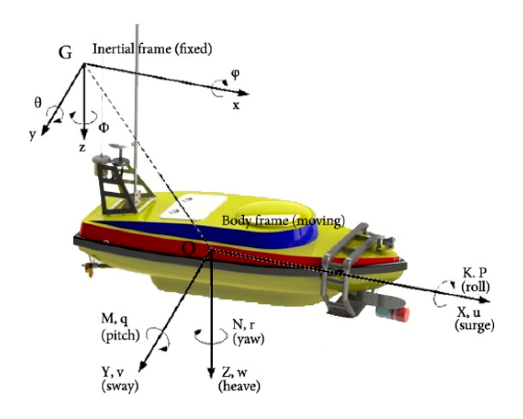
2. USV Dynamics
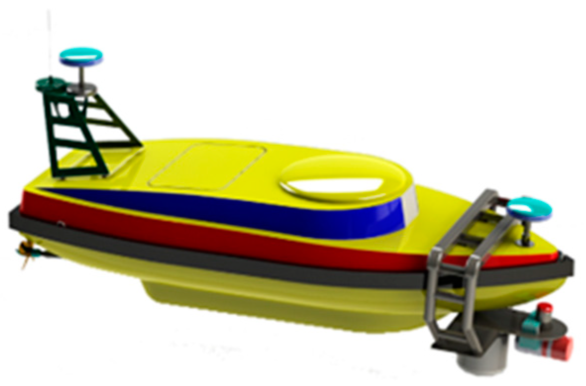
2.1. Deepsea Warriors Uboat (DW-Uboat)
2.2. Assumption
- The motion of the USV in roll, pitch, and heave directions was neglected.
- The USV had neutral buoyancy and the origin of the body-fixed coordinate was located at the center of mass.
- The dynamic equations of the USV did not include the disturbance forces (waves, wind, and ocean currents).
2.3. Dynamic Models
3. PINNs
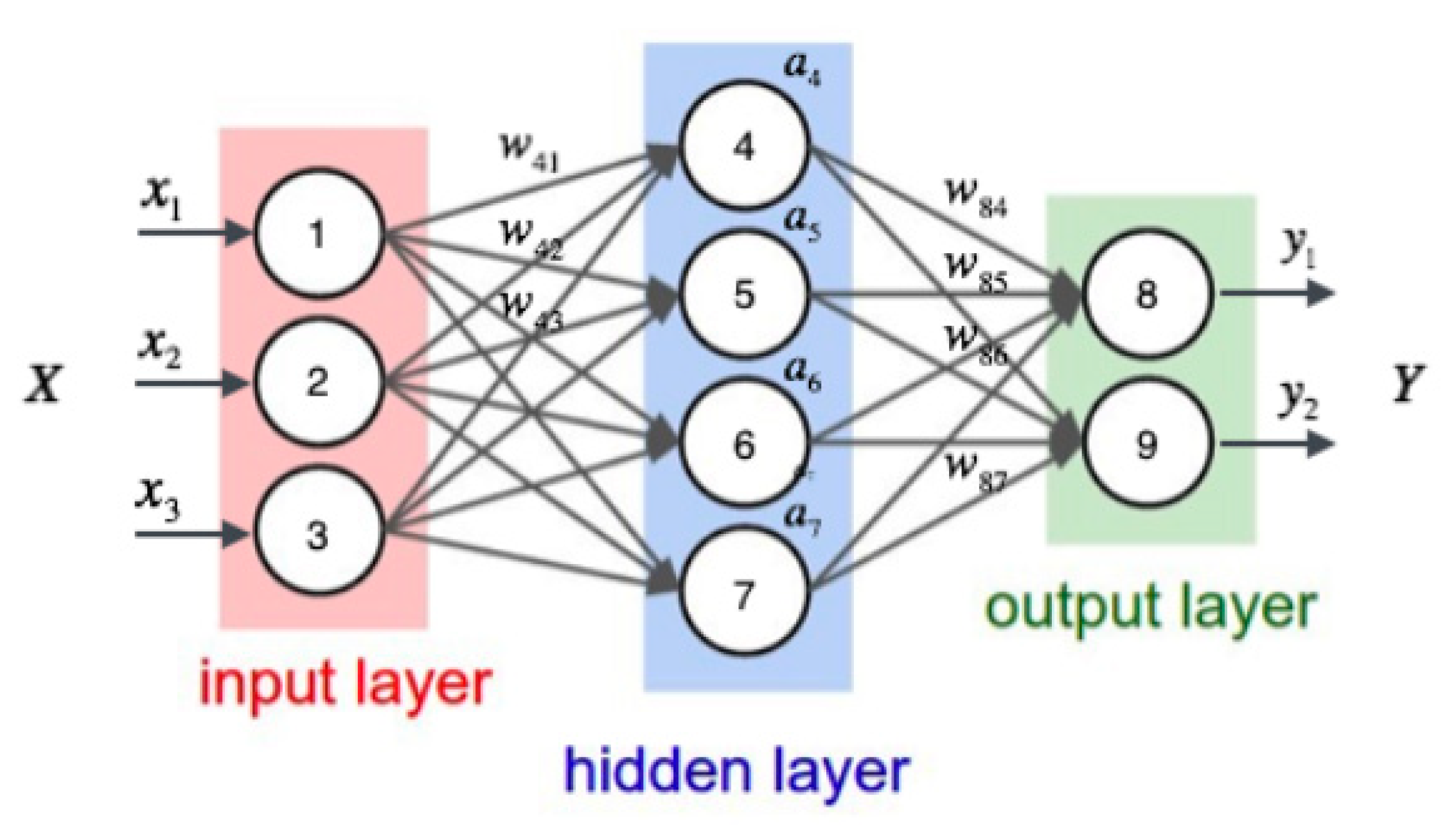
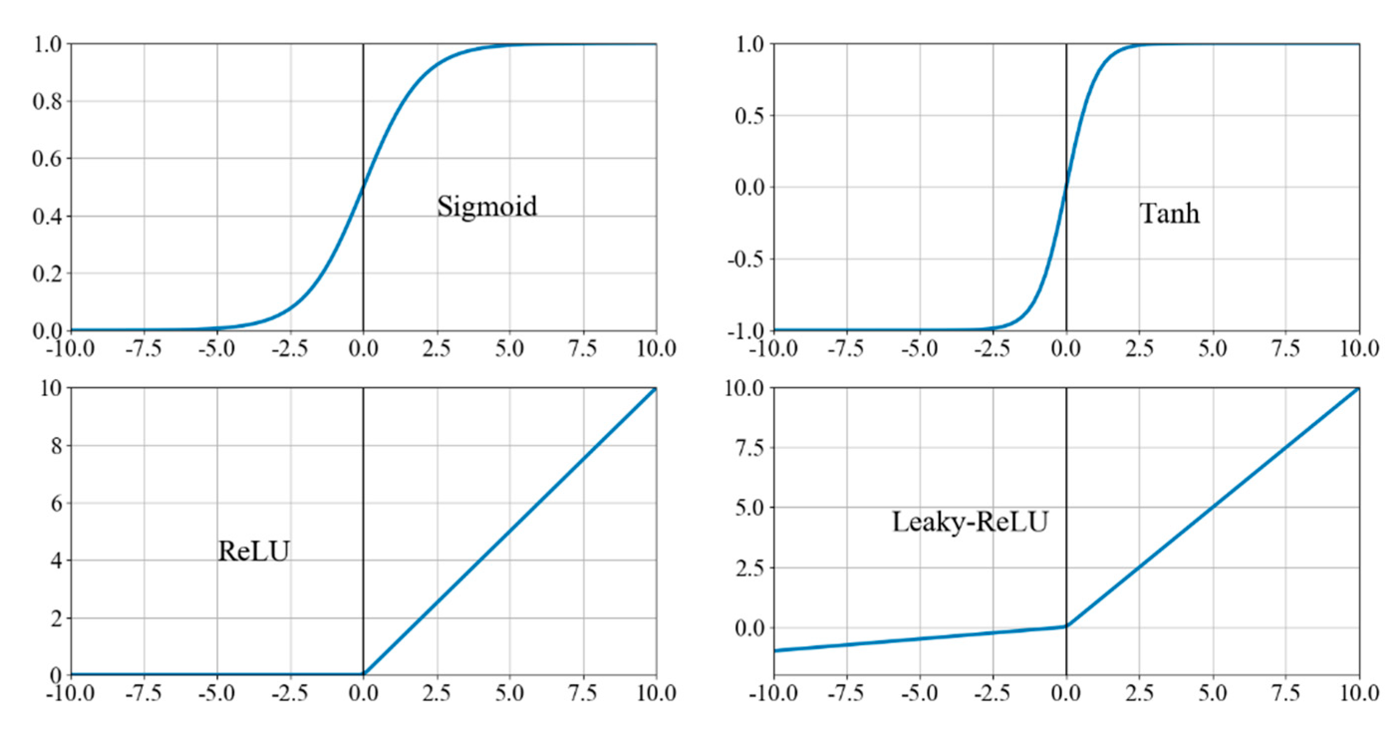
3.1. ANNs
3.2. PINN Method
3.3. PINN for Solving Dynamic Models of the USV
4. Results
4.1. Data Preprocessing
4.2. Identified Results
4.3. PINN Versus Traditional Neural Network
5. Conclusions
Author Contributions
Funding
Data Availability Statement
Acknowledgments
Conflicts of Interest
References
- Fang, Y.; Pang, M.Y.; Wang, B. A course control system of unmanned surface vehicle (USV) using back-propagation neural network (BPNN) and artificial bee colony (ABC) algorithm. In Proceedings of the 8th International Conference on Advances in Information Technology, IAIT2016, Macau, China, 19–22 December 2017. [Google Scholar]
- Fossen, T.I. Marine Control Systems: Guidance, Navigation and Control of Ships, Rigs and Underwater Vehicles; Marine Cybernetics: Trondheim, Norway, 2002. [Google Scholar]
- Woo, T.; Park, J.Y.; Yu, C.; Kim, N. Dynamic model identification of unmanned surface vehicles using deep learning network. Appl. Ocean. Res. 2018, 78, 123–133. [Google Scholar] [CrossRef]
- Sonnenburg, C.R.; Woolsey, C.A. Modeling, identification, and control of an unmanned surface vehicle. J. Field Rob. 2013, 30, 371–398. [Google Scholar] [CrossRef] [Green Version]
- Nagumo, J.I.; Noda, A. A learning method for system identification. IEEE Trans. Autom. Control. AC 1967, 12, 282–287. [Google Scholar] [CrossRef]
- Holzhuter, T. Robust identification scheme in an adaptive track controller for ships. In Proceedings of the 3rd IFAC Symposium on Adaptive System in Control and Signal Processing, Glasgow, UK, 19–21 April 1989; pp. 118–123. [Google Scholar]
- Kallstrom, C.G.; Astrom, K.J. Experiences of system identification applied to ship steering. Automatica 1981, 17, 187–198. [Google Scholar] [CrossRef]
- Yoon, H.K.; Rhee, K.P. Identification of hydrodynamic coefficients in ship maneuvering equations of motion by estimation-before-modeling technique. Ocean Eng. 2003, 30, 2379–2404. [Google Scholar] [CrossRef]
- Shin, J.; Kwak, D.J.; Lee, Y.-I. Adaptive path following control for an unmanned surface vessel using an identified dynamic model. IEEE/ASME Trans. Mechatron. 2017, 22, 1143–1153. [Google Scholar] [CrossRef]
- Selvam, R.P.; Bhattacharyya, S.; Haddara, M. A frequency domain system identification method for linear ship maneuvering. Int. Shipbuild. Prog. 2005, 52, 5–27. [Google Scholar]
- Alattas, K.A.; Mobayen, A.; Din, S.U.; Asad, J.H.; Fekih, A.; Assawinchaichote, W.; Vu, M.T. Design of a Non-Singular Adaptive Integral-Type Finite Time Tracking Control for Nonlinear Systems with External Disturbances. IEEE Access 2020, 9, 102091–102103. [Google Scholar] [CrossRef]
- Vu, M.T.; Thanh, H.N.N.; Huynh, T.T.; Do, Q.T.; Do, T.D.; Hoang, Q.D.; Le, T.H. Station-Keeping Control of a Hovering Over-Actuated Autonomous Underwater Vehicle Under Ocean Current Effects and Model Uncertainties in Horizontal Plane. IEEE Access 2020, 9, 6855–6867. [Google Scholar] [CrossRef]
- Thanh, H.L.N.N.; Vu, M.T.; Mung, N.X.; Nguyen, N.P.; Phuong, N.T. Perturbation Observer-Based Robust Control Using a Multiple Sliding Surfaces for Nonlinear Systems with Influences of Matched and Unmatched Uncertainties. Mathematics 2020, 8, 1371. [Google Scholar] [CrossRef]
- Rajesh, G.; Bhattacharyya, S. System identification for nonlinear maneuvering of large tankers using artificial neural network. Appl. Ocean Res. 2008, 30, 256–263. [Google Scholar] [CrossRef]
- Oskin, D.A.; Dyda, A.A.; Markin, V.E. Neural Network Identification of Marine Ship Dynamics. In Proceedings of the 9th IFAC Conference on Control Applications in Marine Systems. The International Federation of Automatic Control, Osaka, Japan, 17–20 September 2013. [Google Scholar]
- Pan, C.Z.; Lai, X.Z.; Yang, S.X.; Wu, M. An efficient neural network approach to tracking control of an autonomous surface vehicle with unknown dynamics. Expert Syst. Appl. 2013, 40, 1629–1635. [Google Scholar] [CrossRef]
- Hagan, M.T.; Menhaj, M.B. Training feedforward networks with the Marquardt algorithm. IEEE Trans. Neural Netw. 1994, 5, 989–993. [Google Scholar] [CrossRef] [PubMed]
- He, K.; Zhang, X.; Ren, S.; Sun, J. Deep residual learning for image recognition. In Proceedings of the IEEE Conference on Computer Vision and Pattern Recognition, Las Vegas, NV, USA, 27–30 June 2016; pp. 770–778. [Google Scholar]
- Raissi, M.; Perdikaris, P.; Karniadakis, G.E. Physics Informed Deep Learning (Part I): Data-driven Solutions of Nonlinear Partial Differential Equations. arXiv 2017, arXiv:1711.10671. [Google Scholar]
- Xu, P.F.; Cheng, C.; Cheng, H.X.; Shen, Y.L.; Ding, Y.X. Identification-based 3 DOF model of unmanned surface vehicle using support vector machines enhanced by cuckoo search algorithm. Ocean Eng. 2020, 197, 1–11. [Google Scholar] [CrossRef]


| u | Value | v | Value | r | Value |
|---|---|---|---|---|---|
| −0.002 | 0.00237 | 0.000849 | |||
| 0.423 | 0.006043 | −0.00517 | |||
| 0.0992 | −0.54 × 10⁻⁵ | 0.423456 | |||
| −0.00015 | −2.73 × 10⁻⁷ | ||||
| 0.001508 | 0.003286 | ||||
| 0.00211 | 0.003142 | ||||
| −0.00038 | 0.000777 | ||||
| 0.00265 | 0.000105 |
| PINN | Traditional NN | |||||
|---|---|---|---|---|---|---|
| u | v | r | u | V | r | |
| 1000 | ||||||
| 2000 | ||||||
| 3000 | ||||||
| 4000 | ||||||
| 5000 | ||||||
Publisher’s Note: MDPI stays neutral with regard to jurisdictional claims in published maps and institutional affiliations. |
© 2022 by the authors. Licensee MDPI, Basel, Switzerland. This article is an open access article distributed under the terms and conditions of the Creative Commons Attribution (CC BY) license (https://creativecommons.org/licenses/by/4.0/).
Share and Cite
Xu, P.-F.; Han, C.-B.; Cheng, H.-X.; Cheng, C.; Ge, T. A Physics-Informed Neural Network for the Prediction of Unmanned Surface Vehicle Dynamics. J. Mar. Sci. Eng. 2022, 10, 148. https://doi.org/10.3390/jmse10020148
Xu P-F, Han C-B, Cheng H-X, Cheng C, Ge T. A Physics-Informed Neural Network for the Prediction of Unmanned Surface Vehicle Dynamics. Journal of Marine Science and Engineering. 2022; 10(2):148. https://doi.org/10.3390/jmse10020148
Chicago/Turabian StyleXu, Peng-Fei, Chen-Bo Han, Hong-Xia Cheng, Chen Cheng, and Tong Ge. 2022. "A Physics-Informed Neural Network for the Prediction of Unmanned Surface Vehicle Dynamics" Journal of Marine Science and Engineering 10, no. 2: 148. https://doi.org/10.3390/jmse10020148