AIS-Based Scenario Simulation for the Control and Improvement of Ship Emissions in Ports

Abstract

Maritime transport is a major mode of transportation. Over 80% of international freight is carried by this mode. A port is a hub of ships and freight in maritime transport. Because of growing environmental concerns, how to effectively monitor, control, and improve ship emissions in a port has become a challenge for port administrations. This study combines automatic identification systems (AIS), ship emission estimation model (SEEM), geographic information system (GIS) mapping, and a scenario simulation technique to create a ship emission scenario simulation model (SESSM) for mapping and assessing current ship emissions alongside various “what-if” improvement options in a port area. A case study of the Port of Keelung in Taiwan is used to illustrate and verify the proposed model. In this case, the distribution and density of ship carbon emissions are mapped, with the ship berthing status being identified as the primary source of ship emissions. Meanwhile, nine “what-if” scenarios based on various combinations of speed policies and shore power supplies are simulated and analyzed. The results show that the proposed scenario simulation model is an effective tool to assess various “what-if” emission improvement options and to identify key factors for emission reduction. The effect of shore power supply on carbon emission reduction is significantly greater than speed policies. If investment costs are an issue, a balanced emission improvement option is suggested by combining a new speed policy and 50% shore power supply.

1. Introduction

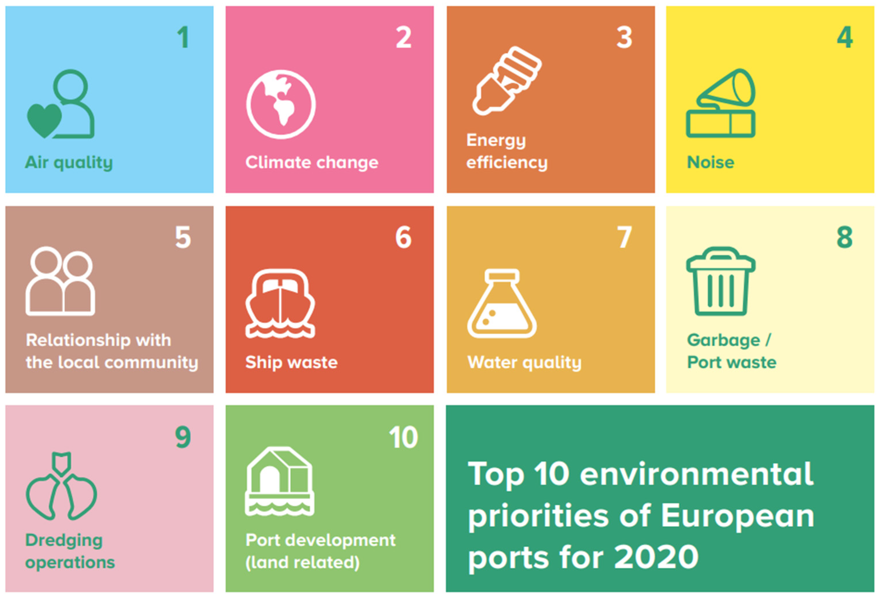
Maritime transport has been the primary transportation mode adopted in global trade. Currently, it transports more than 80% of the world’s freight trade [1]. In maritime transport, ports play a pivotal role, functioning as a hub of ship activities and freight transport across countries. However, this critical function also renders ports a hub of maritime transport pollution. According to the European Sea Ports Organization (ESPO) [2], the top three of the top ten environmental priorities of EU ports in 2020, (1) air quality, (2) climate change, and (3) energy efficiency (see Figure 1), are related to ship emissions at ports. Furthermore, the latest statement from the 2021 United Nations Climate Change Conference (COP 26) indicates that nearly 200 countries agreed to the Glasgow Climate Pact to keep 1.5 °C alive and finalize the outstanding elements of the Paris Agreement [3]. This means that greenhouse gas (GHG) emissions mitigation, adaptation, and financing will come into force in the near future. Additionally, the International Maritime Organization (IMO) also agreed with COP 26 to accelerate its efforts to reduce GHG emissions. IMO’s Marine Environment Protection Committee (MEPC) has begun the revision of the Initial IMO Strategy on reduction in (GHG) emissions from ships [4]. These environmental demands make the monitoring and control of the air pollution in ports a great urgency and a huge challenge not only for ocean carriers but also for port administrations and residents.

The primary sources of air pollution in a port are ocean-going vessels, harbor craft, cargo handling equipment, on-road vehicles, and rail locomotives. Among these sources, vessel emissions are the majority of pollutants [5]. However, pre-existing literature does not propose an effective method for providing instant air emission information of ship activities and “what-if” improvement solutions. This research gap deters the progress of environmental priorities and the control of GHG emissions in the shipping industry. This research aims to develop an instant and effective method able to estimate and to map the emissions of ship activities in a port, as well as to simulate the outcomes of various “what-if” scenarios for decision making if environmental improvement measures are taken.

The fourth IMO GHG study shows that maritime transport emits around 1056 million tons of CO₂ emissions annually and is responsible for about 2.89% of global anthropogenic greenhouse gas GHG emissions [6]. Either for air pollution or GHG control, vessel emissions can simply not be ignored. A considerable amount of literature regarding vessel emissions has been published. For instance, Eyring et al. investigated emissions changes of international maritime shipping from 1950 to 2001. Their results suggest that from 1970 to 2001 the world’s merchant fleet increased rapidly. This fact led to a corresponding increase in total fuel consumption and air pollutants [7]. Endresen et al. studied the environmental impacts of increased international maritime shipping and mapped the geographic distribution of global shipping operations. They showed not only the past trends of emissions but also the future impacts of emissions [8]. In contrast with the worldwide perspective, several researchers have focused on ship emissions in a specific region. Leonardi and Browne presented a method for assessing the carbon footprints of maritime transportation. Based on the data analysis from import supply chains involving several countries in Europe, the results discussed logistics and supply chain choices, the influence of trip distance, load factor, and ship speed [9]. Ammar and Seddiek investigated the case of RO-RO cargo vessels operating in the Red Sea. They compared the environmental and economic performance of four emission reduction methods based on different fuel combinations for ship emission control [10]. Dragović et al. estimated and analyzed ship emission inventories and externalities in the associated cruise bays and ports of Dubrovnik (Croatia) and Kotor (Montenegro) along the eastern coast of the Adriatic Sea. The work also examined port policies for the effective control of air pollutions in such environmentally sensitive areas [11].

In the relevant studies of ship emissions, the method of measuring and estimating ship emissions is a crucial issue and has been widely investigated. Agrawal et al. measured the emissions of the main propulsion engine, auxiliary engine, and an auxiliary boiler on a crude oil tanker and presented a set of emission factors of pollutants. This work provided valuable measurement information for successive studies of ship emission estimation [12]. Corbett et al. adopted a profit-maximizing equation to estimate economically-efficient ship speeds and discussed the policy impacts of a fuel tax and a speed reduction mandate on carbon emissions [13].

Instead of these aforementioned works which rely on static historical shipping statistics for estimating ship emissions, Zaman et al. [14] analyzed realtime ship data in different operational statuses and developed an algorithm to identify the optimum ship speed with the least fuel consumption and carbon emissions.

In recent years, researchers have developed another type of emissions estimation method based on the automatic identification system (AIS). AIS is a tracking system that has been widely used on vessels and can generate navigational data. This type of method adopts the data automatically collected from AIS to estimate the emissions from vessel activities [15,16,17,18]. The primary advantage of the AIS-based method is that an AIS can provide approximately realtime navigational information, which can be applied to other fields, such as emissions monitoring and emissions mapping. The method does not require collecting massive historical shipping statistics in advance. In addition, AIS has been widely installed on various vessels, making additional equipment investment not required. Li et al. [19] presented a high-resolution ship emission inventory for the Pearl River Delta region and showed low uncertainty in utilizing AIS data to improve ship emissions estimates. Chen et al. [20] presented a comprehensive national-scale ship emission inventory in China for 2014 based on AIS data for the full year of 2014.

As mentioned above, vessel emissions are a major source of air pollution in a port. The AIS-based method has been applied to the research on port emissions. For instance, Ng et al. [21] used AIS data to investigate the marine emissions in the neighborhood of Hong Kong and the Pearl River Delta and discussed a potential policy change based on the revealed results. Tichavska and Tovar [22] adopted AIS data to estimate the exhaust pollutants related to ferry and cruise operations by sea in Las Palmas Port. Chen et al. [23] presented a high temporal-spatial ship emission inventory in Qingdao Port and its adjacent waters, also based on AIS data. In addition, Yang et al. [24] and Toscano et al. [25] performed similar studies but considered local issues for Tianjin port and Naples port, respectively. Zhang et al. [26] also used AIS data to estimate the ship emission inventory but focused on unidentified vessels with missing ship parameters. Furthermore, Huang et al. [27] dealt with the needs of real-time ship emission monitoring. They presented a method of dynamic calculation of ship emissions based on real-time ship trajectory data. Weng et al. [28] provided higher spatial-temporal resolution for ship emission estimation.

To date, most of the prior research about maritime emissions based on AIS data focused on macro-scale spatial distribution of ship emissions around the globe or in a broad area of sea or coast, such as the Pearl River Delta, the Yangtze River, the Baltic Sea area, or the Adriatic Sea. Few studies have looked at micro-scale spatial distribution ship emissions in a port. Prior research tends to analyze the existing static condition of air pollution from vessel activities and lacks useful tools to evaluate the emissions in various “what-if” scenarios to identify an appropriate improvement alternative. Instead of analyzing and assessing port emissions in a passive manner, this study introduces the technique of simulation to explore proactive emission improvement alternatives. Few past studies address this issue.

This paper combines historical AIS data, a ship emissions estimation model, and a geographic information system (GIS) to create a scenario simulation model for mapping and assessing ship emissions in a port area. The proposed model can present the distribution and volume of ship emissions not only at current status but also in various “what-if” scenarios. This provides the advantage of realtime environmental monitoring and allows port administration to evaluate which emission improvement alternative performs better.

The rest of this paper is organized as follows: Section 2 describes the study’s framework and method, and Section 3 details the case for analysis and simulation. Section 4 discusses the simulation results using the proposed method. Finally, Section 5 presents the conclusions and potential opportunities for future research.

2. Methods

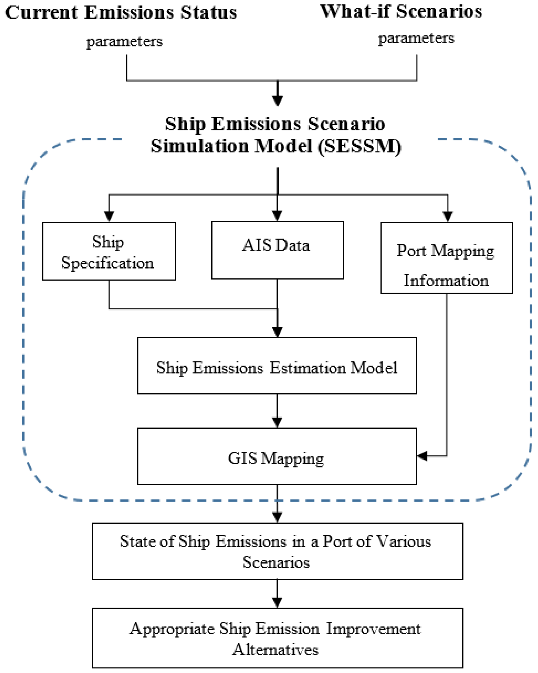
The framework of the proposed method is called Ship Emissions Scenario Simulation Model (SESSM) and is illustrated in Figure 2. It requires three types of input data: ship specifications, AIS data, and port mapping information. Ship specifications include ship size, ship tonnage, and propulsion machine. AIS dynamic data mainly include ship direction, position, speed, etc. These two types of data are the input of the Ship Emissions Estimation Model (SEEM). SEEM uses the data as the basic parameters to estimate the volume of ship emissions. Port mapping information provides the scope of the mapping area of the port for ship emissions monitoring. It is the input of GIS mapping of ship emissions and thus needs to be defined clearly. Combining the output of SEEM and port mapping information, GIS maps the distribution and density of ship emissions in a specific port area. These components form the basic framework of the SESSM. The output of the SESSM can be used either for the illustration of the current ship emission status or for the simulation of different “what-if” scenarios. Furthermore, they can be compared and analyzed to improve the control of ship emissions in a port area and to find appropriate improvement options for ship emission reduction. More details of the framework are described below.

2.1. Automatic Identification System (AIS)

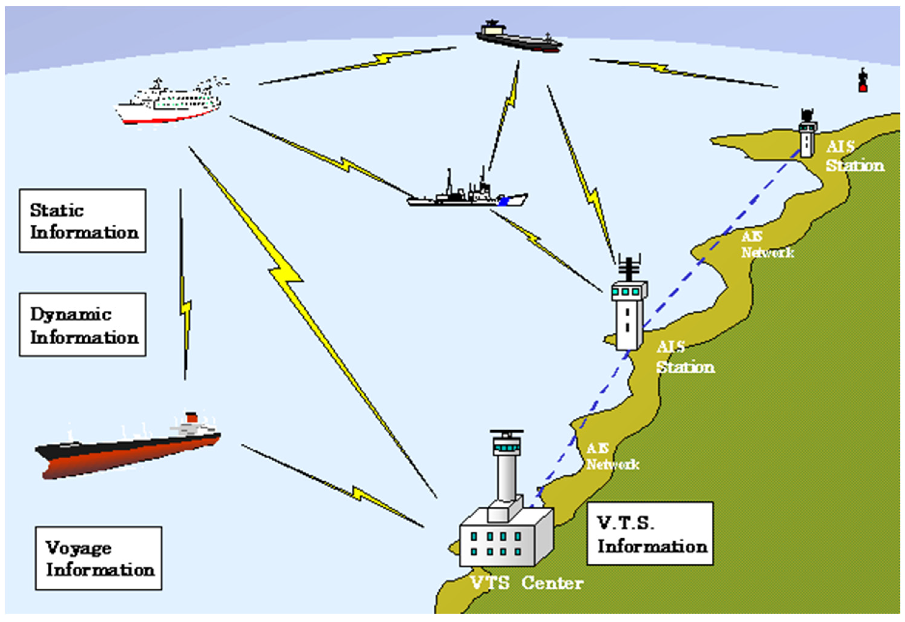
AIS is a tracking system, which has been widely used on ships at sea. The AIS combines Global Positioning System (GPS) and Very High Frequency (VHF) radio communication technology and enables ships to exchange various navigational information in two different modes—ship-to-ship and ship-to-shore—as shown in Figure 3. The main AIS facilities on land include vessel traffic service (VTS) centers and AIS base stations. The broadcast navigational information of the AIS mainly includes three types: static, dynamic, and voyage. The static information contains ship identification number (known as IMO number), length, beam, and ship type. The dynamic information varies with time, frequently containing position, course, speed, heading, etc. The voyage-related information includes hazardous cargo onboard, draft, destination, route plan, etc. Using this information, the AIS can provide various maritime functions, such as collision avoidance, navigation, maritime security, search, and rescue, etc. In this study, the traditional roles of the AIS are expanded to the environmental monitoring of ship activities.

2.2. Ship Emission Estimation Model (SEEM)

Several AIS-based models have been developed to estimate ship emissions [15,16,17,18]. Most of these models calculate ship emissions mainly based on engine activities and energy consumption. This study assesses the emissions of individual ships as a function of vessel energy demand multiplied by an emission factor and fuel correction factor as calculated in Equation (1). This estimation model has been implemented and verified by the port of Los Angeles and the major ports of Taiwan [5,30]. The energy demand is the energy output of engines on a ship, which is measured in kW-hr. It comes from three types of sources: main engines, auxiliary engines, and auxiliary boilers. See Equation (2) below. The energy demand is mainly determined by the maximum continuous rated engine power (MCR), load factor (LF), and activity (Act), as shown in Equations (3)–(5). MCR power is defined as the manufacturer’s tested engine power and related to the highest power available from a ship engine during average cargo and sea conditions. The load factor means propulsion engine load factor and is expressed as the cube of the ratio of a ship’s actual speed to the ship’s maximum speed as calculated in Equation (6). From a practical perspective, operating a ship at 100% of its MCR power is very costly in terms of fuel consumption and engine maintenance. Therefore, at normal service speed, a ship usually has a load factor of close to 80%. The activity refers to propulsion engine activity and is measured in operation hours of an engine as calculated in Equation (7). The calculation of the fuel correction factor in Equation (1) follows

Table A7. Fuel Correction Factor [32].

	NOx	VOC	CO	SO2	PM10	PM2.5	DPM	CO2	N2O	CH4
HFO (2.7%S)	1	1	1	1	1	1	1	1	1	1
HFO (1.5%S)	1	1	1	0.555	0.82	0.82	0.82	1	1	1
MGO (0.5%S)	0.94	1	1	0.185	0.25	0.25	0.25	1		1
MDO (1.5%S)	0.94	1	1	0.555	0.47	0.47	0.47	1		1
MGO (0.1%S)	0.94	1	1	0.037	0.17	0.17	0.17	1		1
MGO (0.3%S)	0.94	1	1	0.111	0.21	0.21	0.21	1		1
MGO (0.4%S)	0.94	1	1	0.148	0.23	0.23	0.23	1		1

in Appendix A.

$$E=Energy\times EF\times FCF/{10}^6$$

(1)

$$Energy=Energ{y}_{me}+Energ{y}_{ae}+Energ{y}_{ab}$$

(2)

$$Energ{y}_{me}=MCR\times L{F}_{me}\times Act$$

(3)

$$Energ{y}_{ae}=MCR\times L{F}_{ae}\times Act$$

(4)

$$Energ{y}_{ab}=L{F}_{ab}\times Act$$

(5)

$$LF={(\frac{AS}{MS})}^3$$

(6)

$$Act=D/AS$$

(7)

The nomenclature used in Equations (1)–(7) is provided below.

• E: Emission (ton);
• Energy: Total energy demand (kW-hrs);
• Energy_me: Energy demand of a main engine (kW-hrs);
• Energy_ae: Energy demand of an auxiliary engine (kW-hrs);
• Energy_ab: Energy demand of an auxiliary boiler (kW-hrs);
• MCR: Maximum continuous rating power (kW);
• LF_me: Load factor of a main engine;
• LF_ae: Load factor of an auxiliary engine;
• LF_ab: Load factor of an auxiliary boiler;
• Act: Activity (hrs);
• EF: Emission factor (g/kW-hrs);
• FCF: Fuel correction factor;
• AS: Actual speed (knots);
• MS: Maximum speed (knots); and
• D: Distance (nautical miles).

Ship emissions contain various types of pollutants as shown in Appendix A 

Table A4. Main Engine Emission Factors (Unit: g/kWh) [32].

Model Year	NOx	VOC	CO	SO2	PM10	PM2.5	DPM	CO2	N2O	CH4
<=1999	14	0.5	1.1	11.5	1.5	1.2	1.5	683	0.031	0.01
2000–2010	13	0.5	1.1	11.5	1.5	1.2	1.5	683	0.031	0.01
2011–2015	10.5	0.5	1.1	11.5	1.5	1.2	1.5	683	0.031	0.01

, such as 10-μm micron particulate matter (PM10), 2.5-μm particulate matter (PM2.5), oxides of nitrogen (NO_x), oxides of sulfur (SO_x), carbon monoxide (CO), etc. Because of intensive concerns on the global impact of the greenhouse effect and climate change in recent years, this study focuses on GHGs, and the results present only one type of emission, carbon dioxide equivalent (CO_2e). However, using the Table A4,

Table A5. Auxiliary Engine Emission Factors (Unit: g/kWh) [32].

Model Year	NOx	VOC	CO	SO2	PM10	PM2.5	DPM	CO2	N2O	CH4
<=1999	14.7	0.5	1.1	12.3	1	0.8	1	683	0.031	0.008
2000–2010	13	0.5	1.1	12.3	1	0.8	1	683	0.031	0.008
2011–2015	10.5	0.5	1.1	12.3	1	0.8	1	683	0.031	0.008

and

Table A6. Auxiliary Boiler Emission Factors (Unit: g/kWh) [32].

NOx	VOC	CO	SO2	PM10	PM2.5	DPM	CO2	N2O	CH4
2.1	0.1	0.2	16.5	0.8	0.6	0	970	0.08	0.002

in Appendix A, the other pollutants can be easily estimated, and other indicators or multilayer mapping can also be easily applied in the proposed model.

The static information of AIS data, such as IMO ship identification number, can help us identify critical ship characteristics, such as ship tonnage and power sources. Moreover, the dynamic information of AIS data can provide other critical parameters, such as position and speed. These parameters enable SEEM to effectively estimate the emissions of a ship during different times.

2.3. Geographic Information System (GIS)

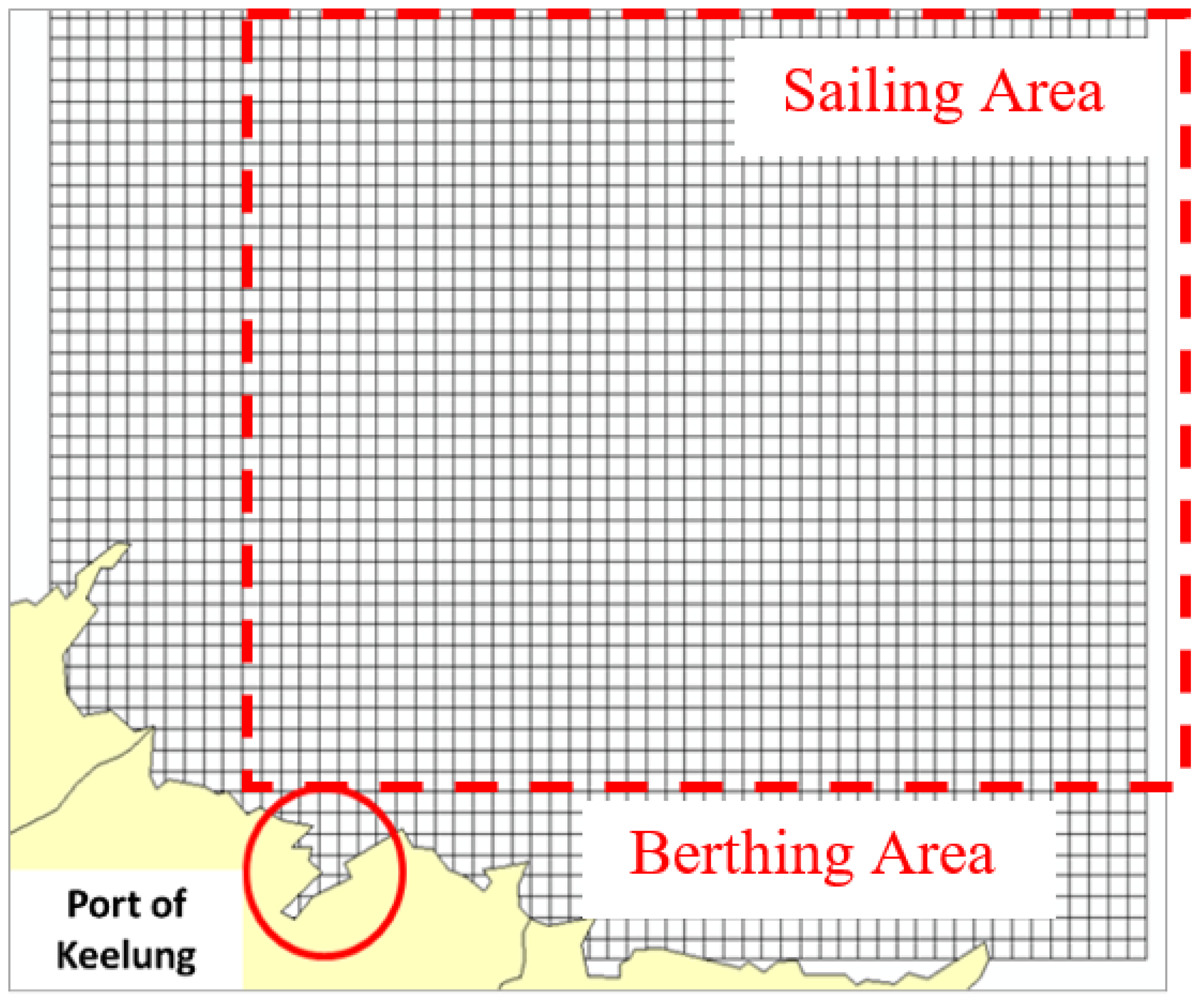
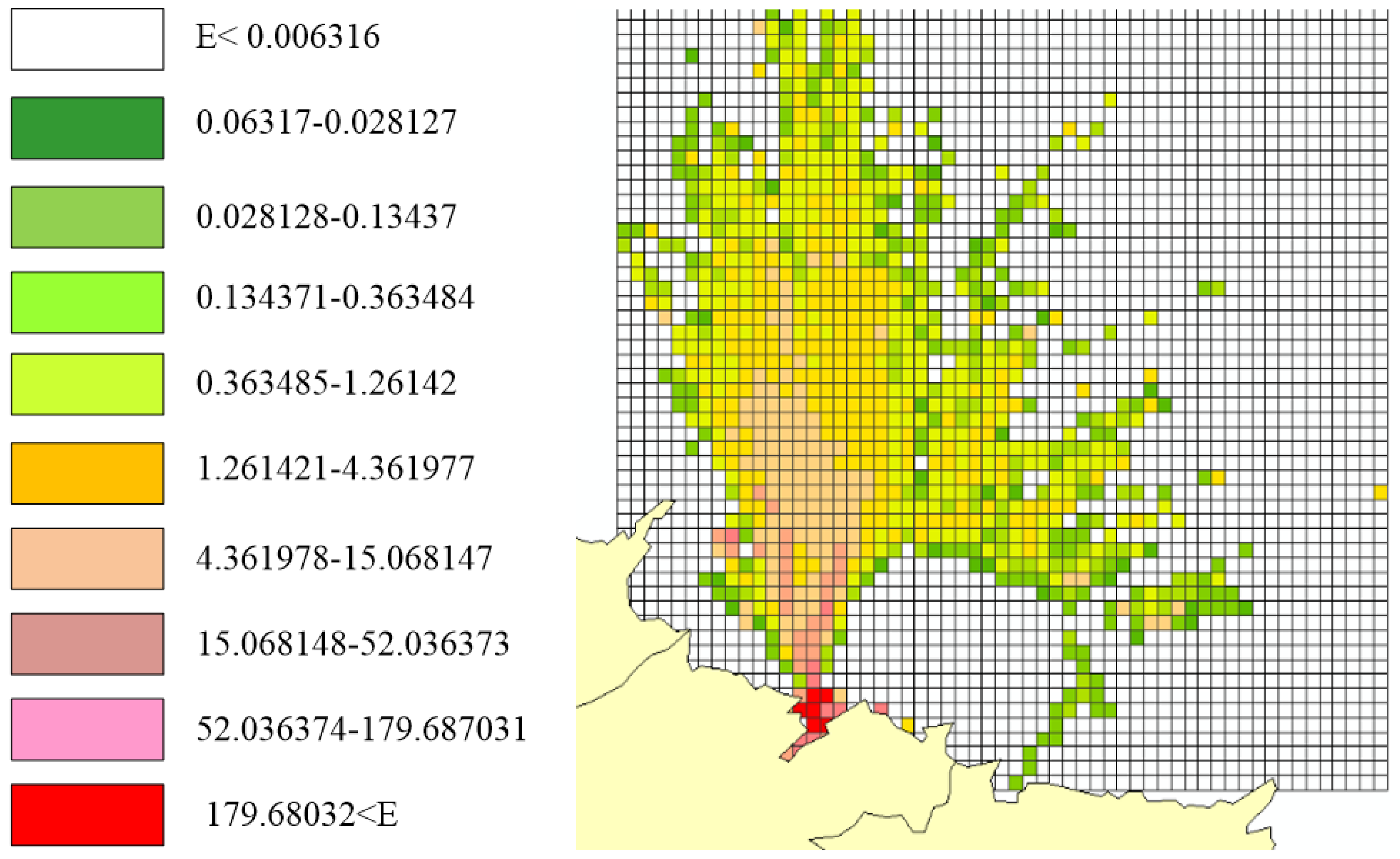
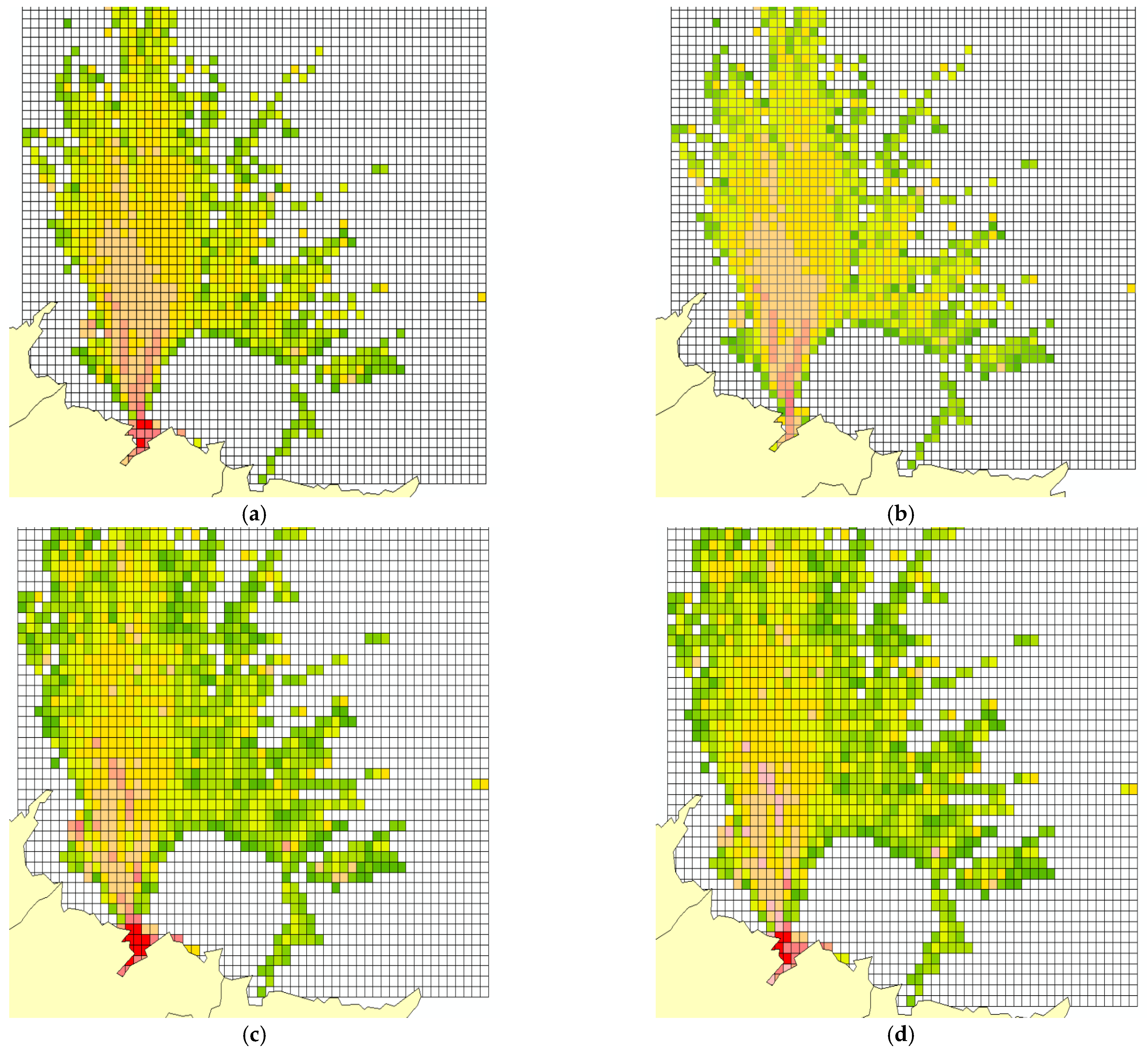
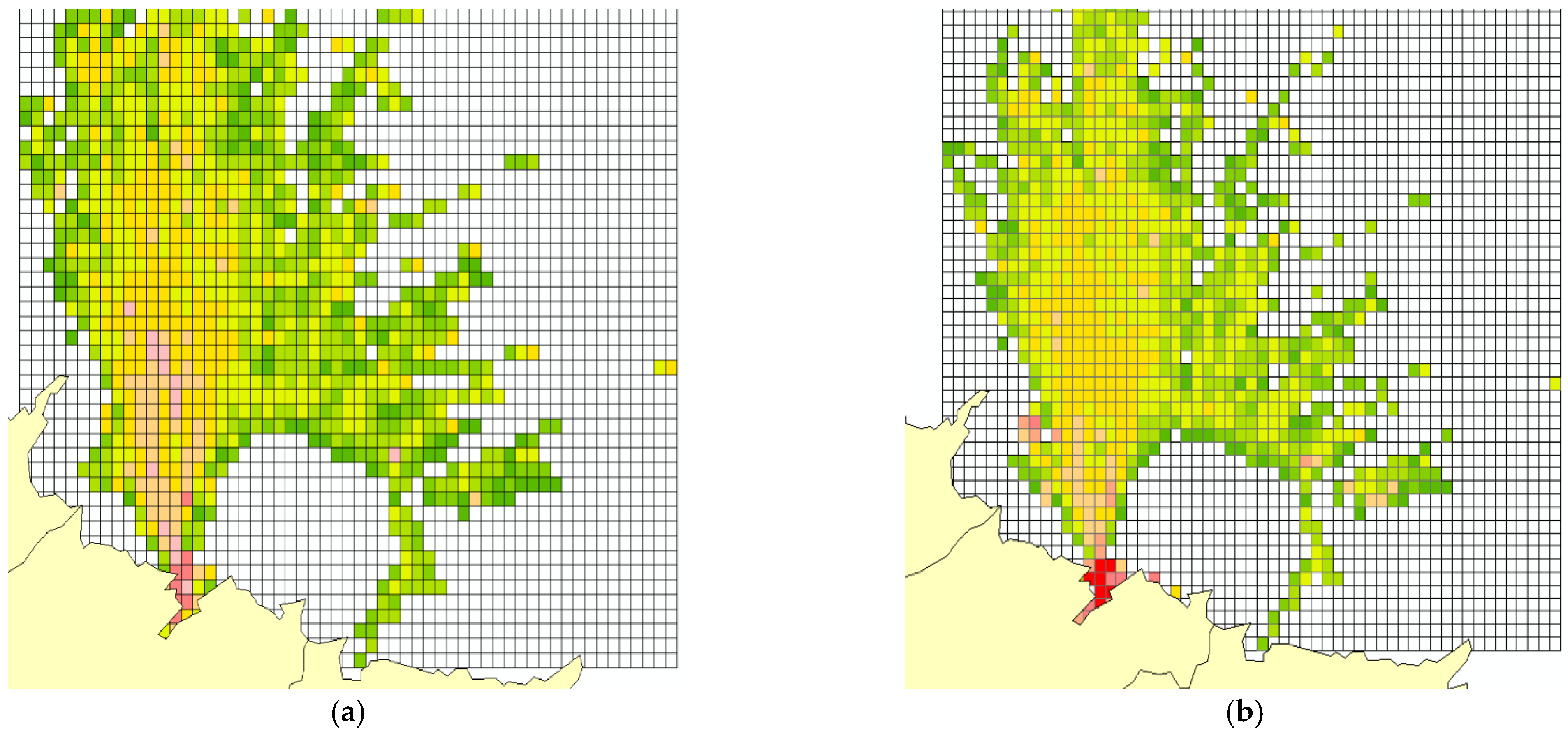
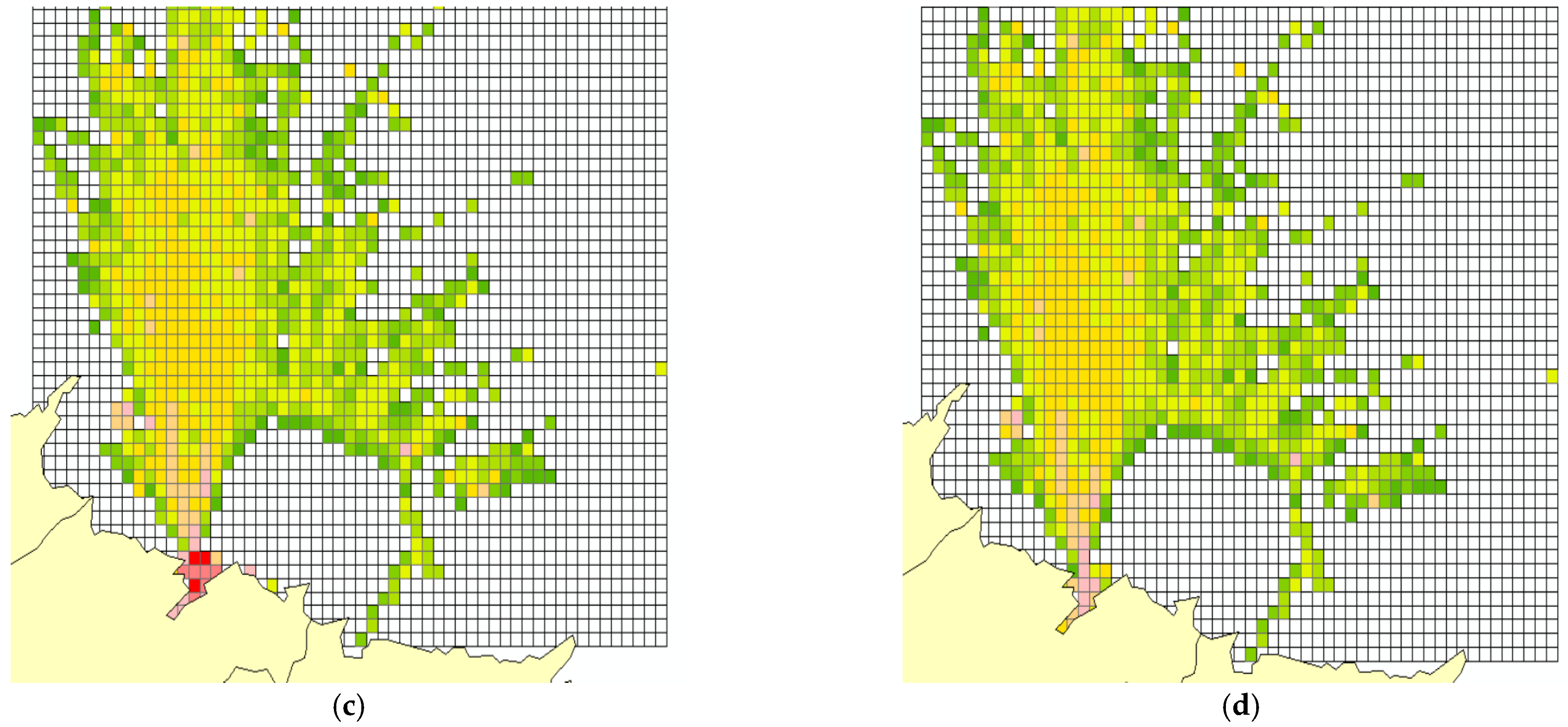
GIS is a system used to create, analyze, manage, and present various geographic data on a map. It has been widely applied in different fields, including traffic navigation, real estate, national defense, natural resources, etc. Based on the data of ship emissions estimated by SEEM, the GIS in the study is used to visualize the distribution of ship emissions in a port area and to simulate “what-if” scenarios of emissions improvement options. The GIS software used in the paper is ArcMap 10, which maps the port area in grids and plots the density of ship emissions in different colors.

3. Case

3.1. The Port of Keelung

The focus point of this study is the Port of Keelung, a major port in northern Taiwan established in 1886, at 25.1346° N, 121.7411° E (see Figure 4). The Port of Keelung handles about 1.53 million TEU containers and 63 million tons of cargo annually [31]. The AIS data in the study were collected by the AIS base stations around the port in June 2015, including 425 individual ships. Ship status includes sailing on the sea, maneuvering, and berthing. The geographical domain designed for monitoring in the port is the square zone within the range of 20 nautical miles (NM) outside the center of the port, as indicated in Figure 4. The site is plotted in a grid with 500-meter intervals, as shown in Figure 5. The berthing area is the circle area at the bottom of Figure 5.

3.2. “What-If” Scenarios of Ship Emissions Improvement Plans

In addition to presenting the current status of ship emissions, evaluating various ship emissions improvement plans is another crucial issue in this study. Presently, there are several common measures for vessel air pollution prevention in international port administrations, such as the use of shore power, the use of low-sulfur fuels, the decrease in vessel speed, etc. This study selected vessel speed policy and the use of shore power as key improvement factors with which to construct nine different “what-if” scenarios. Each factor had three options or levels, as shown in

Table 1. Description of improvement factors.

Improvement Factors	Options/Levels	Remark
Vessel Speed Policy	<20 NM: 12 knots	Current speed policy
	<20 NM: 10 knots	Speed policy 1
	<10 NM: 7 knots
	<20 NM: 12 knots	Speed policy 2
	<15 NM: 10 knots
	<10 NM: 8 knots
	<5 NM: 5 knots
Shore Power Supply	0%	Current facility status
	50%
	100%

and

Table 2. What-if scenarios based on improvement factors.

Scenarios	Improvement Factors
	Speed Policy	Shore Power Supply
1	Current Speed Policy	0%
2	Current Speed Policy	50%
3	Current Speed Policy	100%
4	Speed Policy 1	0%
5	Speed Policy 1	50%
6	Speed Policy 1	100%
7	Speed Policy 2	0%
8	Speed Policy 2	50%
9	Speed Policy 2	100%

.

In Table 1, the first factor, “Vessel Speed Policy,” included three different options: (1) current port speed policy, (2) speed policy 1, and (3) speed policy 2. The “current speed policy” is the speed policy that is being implemented by the Port of Keelung. As shown in Figure 6, it requests the ships to decrease their speed to under 12 knots within the port area (<20 NM). The other two options are “what-if” speed policies for improving emissions. The “speed policy 1” and “speed policy 2” are stepwise speed policies that request ships to decrease the speed at different levels within different distance ranges from the port, as shown in Table 1 and Figure 7 and Figure 8.

In Table 1, the second factor, “Shore Power Supply,” has three different levels: 0%, 50%, and 100%. These levels indicate the percentage of onshore power the berthed ships in a port use. Currently, the Port of Keelung has very few facilities providing shore power to berthing ships. Thus, 0% is close to the current status of power supply. The other two levels, 50% and 100%, are “what-if: plans for improving emissions. Because we did not have enough information about how many percentages of berthing ships would turn on their auxiliary boilers, we assumed that berthing ships do not produce emissions for easy estimation. Combining the two factors and their three options (or levels), Table 2 constructs nine “what-if” scenarios. The proposed SESSM can provide the emissions outcomes in the current situation and the “what-if” scenarios.

4. Results and Discussions

Based on the proposed SESSM methodology, Figure 9, Figure 10 and Figure 11 illustrate the simulation result of the distribution and density of carbon emissions in the nine different scenarios in the port area of Keelung. The colors in the grid (500 × 500 m²) represent the density of carbon emissions. Density is indicated (from low to high) as white, dark green, light green, yellow, orange, and red. The density indicator of carbon emissions (ton per cell in the grid) for different colors is presented in Figure 9.

4.1. Vessel Speed Policy

Figure 9 and Figure 10a–d and Figure 11a–d represent three sets of scenarios for the three speed policies. Scenarios 1–3 followed the current speed policy, Scenarios 4–6 followed speed policy 1, and Scenarios 7–9 followed speed policy 2. We can observe that the speed policies have a significant impact on the distribution and density of ship carbon emissions in the sailing area of the port. The sailing area of the port in Figure 9 and Figure 10a,b has more dense red and orange cells than Figure 10c,d and Figure 11a. Figure 11b–d have more dense green and yellow cells than the other figures (i.e., Figure 9, Figure 10 and Figure 11a). This indicates that the proposed stepwise speed policies are environmental friendly, producing less carbon emission than the current speed policy during sailing status. Speed policy 2, which has more interval speed reduction, performs better than speed policy 1 in carbon emissions.

4.2. Shore Power Supply

Figure 9, Figure 10c and Figure 11b are the scenarios showing the current port facility status. Figure 10a,d and Figure 11c are the simulation scenarios for shore power levels of 50%, and Figure 10b and Figure 11a,d are the simulation scenarios for shore power levels of 100%. Obviously, the current port status has red cells concentrated in the berthing area, indicating the existing port facilities do not supply any power to berthing ships. It causes ships to produce serious carbon emissions staying in the berthing area. If the shore power level increases to 50%, the number of red cells decreases. This simulation result tells that the ship carbon emissions can be reduced significantly. If the shore power level increases to 100%, the red cells all turn orange or yellow indicating that the ship emissions are improved further. However, the maneuvering activities of the ships in the berthing area still produce a tremendous amount of carbon emissions. This means the cells will not turn completely green.

4.3. Volume of Ship Emissions

Figure 12 shows the total volume of ship carbon emissions and the emissions volume of different ship statuses (sailing and berthing) in various scenarios. Scenario 1, the current port status, has the highest carbon emissions, and Scenario 9 has the lowest carbon emissions. Scenarios 3, 6, and 9 simulate 100% shore power supply, so emissions at the berthing status (grey portion) are zero.

Table 3. The influence of improvement factors on ship carbon emissions in different scenarios.

Scenarios	Composition %		Influence Factors
	Sailing and Maneuvering	Berthing	Speed Policy	Shore Power	Emissions Difference
1	36.6%	63.4%	--	--	current status
2	53.6%	46.4%	--	50%	−31.7%
3	100.0%	0.0%	--	100%	−63.4%
4	29.8%	70.2%	policy 1	--	−9.7%
5	45.9%	54.1%	policy 1	50%	−41.4%
6	100.0%	0.0%	policy 1	100%	−73.1%
7	23.4%	76.6%	policy 2	--	−17.2%
8	37.9%	62.1%	policy 2	50%	−48.9%
9	100.0%	0.0%	policy 2	100%	−80.6%

presents the composition percentage of carbon emissions during sailing and berthing and the influence of the improvement factors, speed policy, and shore power. In the current port status (Scenario 1), carbon emissions generated by sailing and maneuvering are about one-third (36.6%), and those generated by berthing are about two-thirds (63.4%). This indicates that in our mapping area, berthing is the major source of carbon emissions. If the shore power supply increases to 50%, as in Scenario 2, about one-third of the total carbon emissions (31.7%) can be reduced. Suppose the shore power supply increases to 100%, as in Scenario 3, all emissions during berthing can be reduced. That means that two-thirds of the total emission (63.4%) can be reduced simply by using shore power. Therefore, the implementation of shore power is a critical measure for the reduction in carbon emissions in a port area.

Because emissions for sailing and maneuvering account for only 36.6%, positive results from a speed policy are much less than those of providing shore power supply. If speed policy 1 is implemented, as outlined in Scenario 4, total emissions can be reduced less than 10%. If speed policy 2 is implemented, as in Scenario 7, less than 18% of total emissions can be reduced. Comparing the two speed policies, the contribution of speed policy 2 to the reduction in total ship carbon emissions is almost double (17.2% vs. 9.7%). Obviously, speed policy 2 outperforms speed policy 1 in emissions reduction.

Presently, the port has insufficient shore power facilities. Since the installation of shore power facilities would require an extra investment cost, increasing the shore power supply to 100% may not be achievable in a short time. Thus, an initial change to 50% shore power supply is a reasonable improvement target. Scenario 8, the improvement option combining speed policy 2 and shore power 50%, is the best one among all 50% shore power options, as it can reduce the most carbon emissions—almost half of the total emissions (48.9%).

5. Conclusions

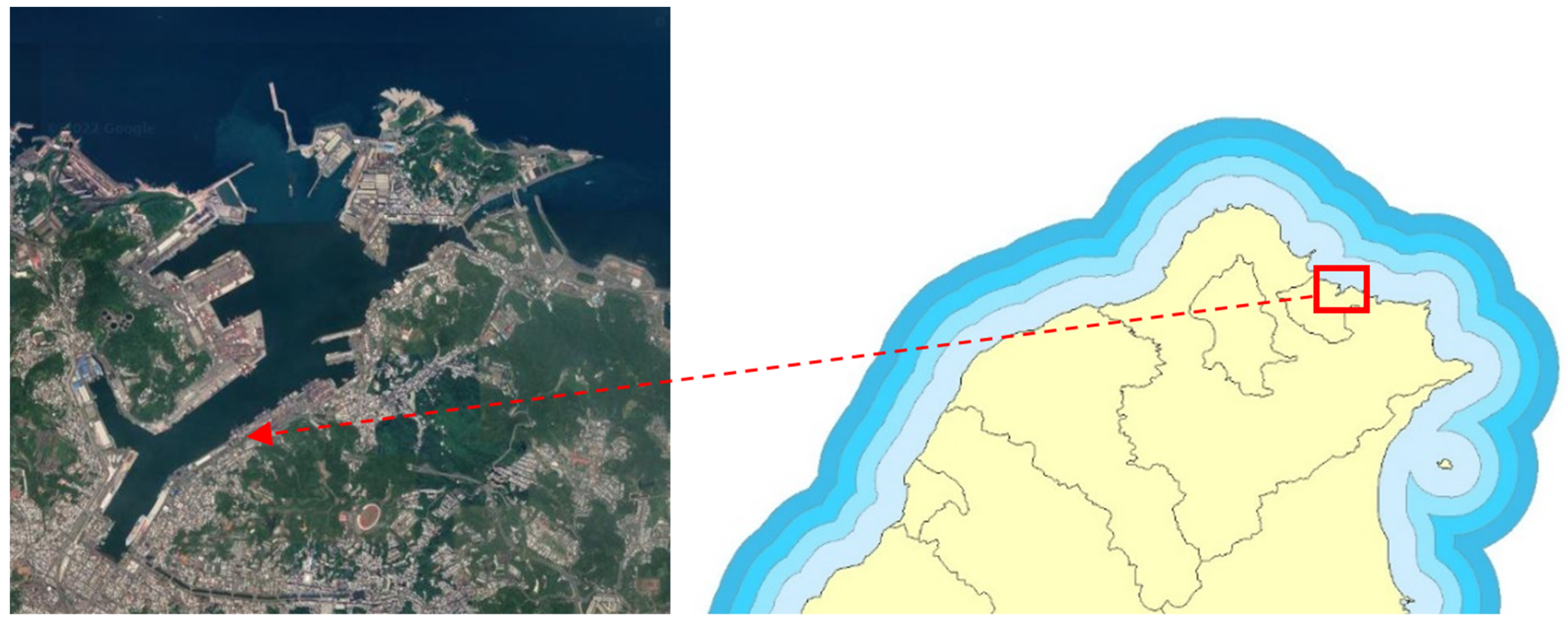
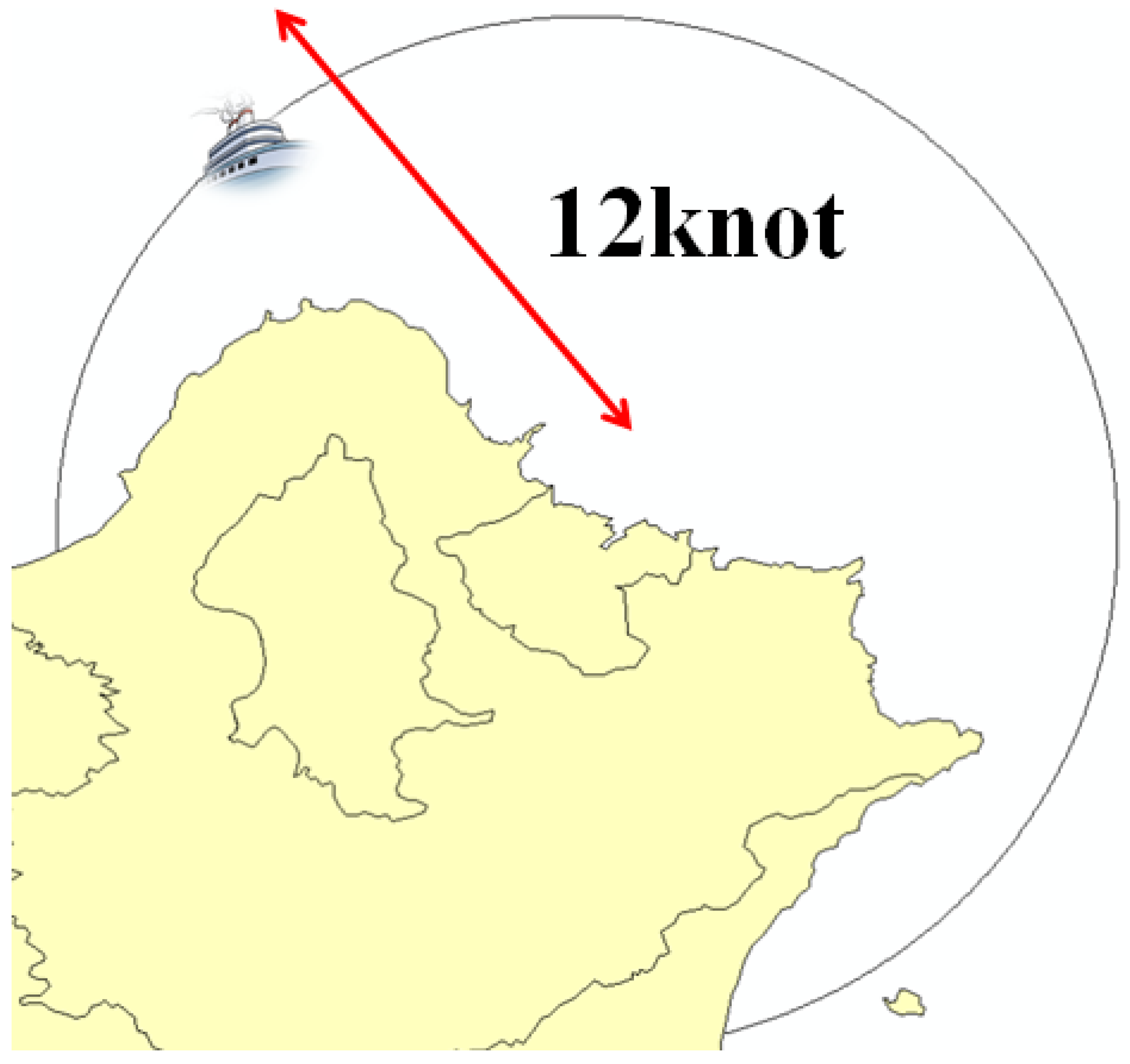
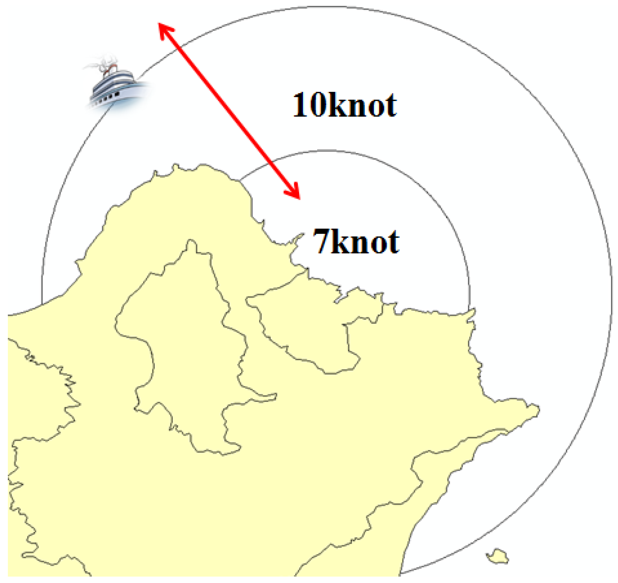
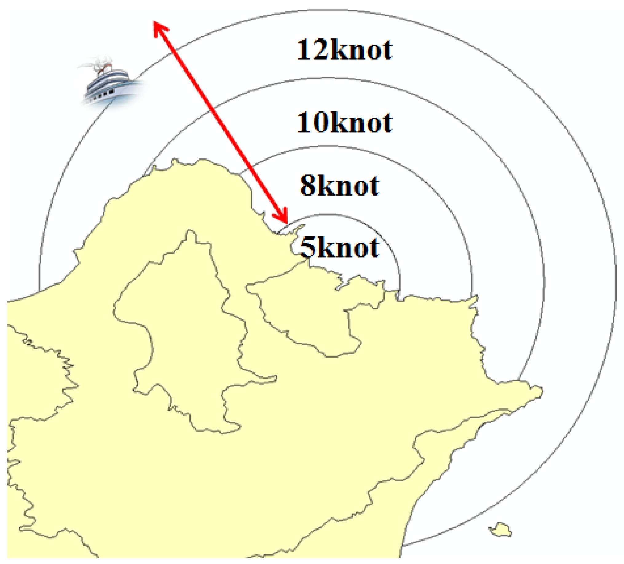
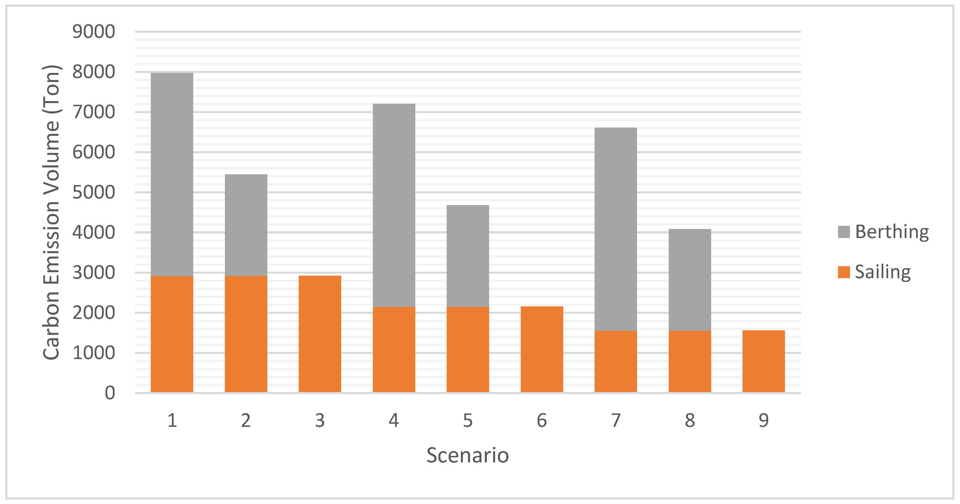
This paper combined AIS, SEEM, GIS mapping, and a scenario simulation technique to construct a ship emissions scenario simulation model for mapping and assessing the ship emissions of the current status and “what-if” improvement scenarios in a port area. The proposed model successfully mapped and estimated the distribution and density of the Port of Keelung and simulated the other “what-if” improvement scenarios. The results show that SESSM is an effective tool to assess various “what-if” emission improvement options and is able to identify key factors for emission reduction. Based on the case study of the Port of Keelung, the primary source of ship carbon emissions comes from ship berthing status. Thus, the improvement of shore power supply can reduce total ship emissions significantly, especially in the area of the berthing docks. However, this improvement incurs a great number of investment costs. The change of speed policies affects emissions less than the shore power supply does but will not require additional investment costs from port administrations. The improvement option balancing the two factors seems to be the best initial option.

Since the proposed simulation model is innovative to the relevant study of ship emissions control, it may not be sufficiently refined. Many issues have not been fully addressed and need to be perfected in future work. For instance, the simulation model is deterministic. Other critical variables, such as investment costs, operation costs, maintenance costs, weather, and sea conditions have not been considered. A complicated simulation model involving these stochastic and realistic elements can be developed to provide further financial analysis for port planning evaluation. In addition, the scenarios include only two improvement factors—speed policies and shore power supply. If relevant data iare available, more experiment factors and levels can be added into the simulation scenarios to provide port administrations with more feasible and flexible options for decision making.

References

1. IMO (International Maritime Organization). Introduction to IMO. Available online: http://www.imo.org/en/About/Pages/Default.aspx (accessed on 24 November 2021).
2. ESPO. Top 10 Environmental Priorities of EU Ports 2020. EcoPorts Publications. 2020. Available online: https://www.ecoports.com/publications/top-10-environmental-priorities-of-eu-ports-2020 (accessed on 24 November 2021).
3. COP26. United Nations Climate Change Conference. 2021. Available online: https://ukcop26.org/cop26-keeps-1-5c-alive-and-finalises-paris-agreement/ (accessed on 24 November 2021).
4. Marine Environment Protection Committee (MEPC) 77, IMO. 2021. Available online: https://www.imo.org/en/MediaCentre/MeetingSummaries/Pages/MEPC77.aspx (accessed on 12 December 2021).
5. Starcrest Consulting Group, LLC. Port of Los Angeles Port of Los Angeles Inventory of Air Emission—2014. 2015. Available online: https://kentico.portoflosangeles.org/getmedia/8066ecf3-86a1-4fa8-b1c9-f9726b92be67/2014_Air_Emissions_Inventory_Full_Report (accessed on 18 November 2021).
6. Forth Greenhouse Gas Study, IMO. 2020. Available online: https://www.imo.org/en/OurWork/Environment/Pages/Fourth-IMO-Greenhouse-Gas-Study-2020.aspx (accessed on 12 December 2021).
7. Eyring, V.; Köhler, H.; van Aardenne, J.; Lauer, A. Emissions from international shipping: 1. The last 50 years. J. Geophys. Res. D Atmos. 2005, 110, D17. [Google Scholar] [CrossRef]
8. Endresen, Ø.; Dalsøren, S.; Eide, M.; Isaksen, I.S.; Sørgård, E. The environmental impacts of increased international maritime shipping–Past trends and future perspectives. In Proceedings of the Global Forum on Transport and Environment in a Globalising World, Guadalajara, Mexico, 10 November 2008. [Google Scholar]
9. Leonardi, J.; Browne, M. A method for assessing the carbon footprint of maritime freight transport: European case study and results. Int. J. Logist. Res. Appl. 2010, 13, 349–358. [Google Scholar] [CrossRef]
10. Ammar, N.R.; Seddiek, I.S. Eco-environmental analysis of ship emission control methods: Case study RO-RO cargo vessel. Ocean Eng. 2017, 137, 166–173. [Google Scholar] [CrossRef]
11. Dragović, B.; Tzannatos, E.; Tselentis, V.; Meštrović, R.; Škurić, M. Ship emissions and their externalities in cruise ports. Transp. Res. D Transp. Environ. 2018, 61, 289–300. [Google Scholar] [CrossRef]
12. Agrawal, H.; Welch, W.A.; Miller, J.W.; Cocker, D.R. Emission measurements from a crude oil tanker at sea. Environ. Sci. Technol. 2008, 42, 7098–7103. [Google Scholar] [CrossRef] [PubMed] [Green Version]
13. Corbett, J.J.; Wang, H.; Winebrake, J.J. The effectiveness and costs of speed reductions on emissions from international shipping. Transp. Res. D Transp. Environ. 2009, 14, 593–598. [Google Scholar] [CrossRef]
14. Zaman, I.; Pazouki, K.; Norman, R.; Younessi, S.; Coleman, S. Utilising real-time ship data to save fuel consumption and reduce carbon emission. In Shipping in Changing Climates Conference; Newcastle University: Newcastle, UK, 2016. [Google Scholar]
15. Perez, H.M.; Chang, R.; Billings, R.; Kosub, T.L. Automatic identification systems (AIS) data use in marine vessel emission estimation. In Proceedings of the 18th Annual International Emission Inventory Conference, Baltimore, MD, USA, 14–17 April 2009. [Google Scholar]
16. Jalkanen, J.-P.; Brink, A.; Kalli, J.; Pettersson, H.; Kukkonen, J.; Stipa, T. A modelling system for the exhaust emissions of marine traffic and its application in the Baltic Sea area. Atmos. Chem. Phys. 2009, 9, 9209–9223. [Google Scholar] [CrossRef] [Green Version]
17. Miola, A.; Ciuffo, B. Regulating Air Emissions from Ships-The State of the Art on Methodologies, Technologies and Policy Options; Institute for Environment and Sustainability, European Commission, Joint Research Centre: Luxembourg, 2010. [Google Scholar]
18. Jalkanen, J.-P.; Johansson, L.; Kukkonen, J.; Brink, A.; Kalli, J.; Stipa, T. Extension of an assessment model of ship traffic exhaust emissions for particulate matter and carbon monoxide. Atmos. Chem. Phys. 2012, 12, 2641–2659. [Google Scholar] [CrossRef] [Green Version]
19. Li, C.; Yuan, Z.; Ou, J.; Fan, X.; Ye, S.; Xiao, T.; Shi, Y.; Huang, Z.; Ng, S.K.; Zhong, Z. An AIS-based high-resolution ship emission inventory and its uncertainty in Pearl River Delta region, China. Sci. Total Environ. 2016, 573, 1–10. [Google Scholar] [CrossRef] [PubMed]
20. Chen, D.; Wang, X.; Li, Y.; Lang, J.; Zhou, Y.; Guo, X.; Zhao, Y. High-spatiotemporal-resolution ship emission inventory of China based on AIS data in 2014. Sci. Total Environ. 2017, 609, 776–787. [Google Scholar] [CrossRef] [PubMed]
21. Ng, S.K.; Loh, C.; Lin, C.; Booth, V.; Chan, J.W.; Yip, A.C.; Li, Y.; Lau, A.K. Policy change driven by an AIS-assisted marine emission inventory in Hong Kong and the Pearl River Delta. Atmos. Environ. 2013, 76, 102–112. [Google Scholar] [CrossRef]
22. Tichavska, M.; Tovar, B. Port-city Exhaust Emission Model: An approach to Cruise and Ferry operations in Las Palmas Port. In Proceedings of the IAME Conference, Norfolk, VA, USA, 15–18 July 2014. [Google Scholar]
23. Chen, D.; Wang, X.; Nelson, P.; Li, Y.; Zhao, N.; Zhao, Y.; Lang, J.; Zhou, Y.; Guo, X. Ship emission inventory and its impact on the PM2. 5 air pollution in Qingdao Port, North China. Atmos. Environ. 2017, 166, 351–361. [Google Scholar] [CrossRef]
24. Yang, L.; Zhang, Q.; Zhang, Y.; Lv, Z.; Wang, Y.; Wu, L.; Feng, X.; Mao, H. An AIS-based emission inventory and the impact on air quality in Tianjin port based on localized emission factors. Sci. Total Environ. 2021, 783, 146869. [Google Scholar] [CrossRef]
25. Toscano, D.; Murena, F.; Quaranta, F.; Mocerino, L. Assessment of the impact of ship emissions on air quality based on a complete annual emission inventory using AIS data for the port of Naples. Ocean Eng. 2021, 232, 109166. [Google Scholar] [CrossRef]
26. Zhang, Y.; Fung, J.C.; Chan, J.W.; Lau, A.K. The significance of incorporating unidentified vessels into AIS-based ship emission inventory. Atmos. Environ. 2019, 203, 102–113. [Google Scholar] [CrossRef]
27. Huang, L.; Wen, Y.; Zhang, Y.; Zhou, C.; Zhang, F.; Yang, T. Dynamic calculation of ship exhaust emissions based on real-time AIS data. Transp. Res. Part D Transp. Environ. 2020, 80, 102277. [Google Scholar] [CrossRef]
28. Weng, J.; Shi, K.; Gan, X.; Li, G.; Huang, Z. Ship emission estimation with high spatial-temporal resolution in the Yangtze River estuary using AIS data. J. Clean. Prod. 2020, 248, 119297. [Google Scholar] [CrossRef]
29. Bright Hub Engineering. Automatic Identification System for Tracking Ships. 2010. Available online: https://www.brighthubengineering.com/seafaring/63389-tracking-ships-using-automatic-identification-system/ (accessed on 12 December 2021).
30. Wang, W.-C. Analytical Utilization of AIS Data in Estimating Fuel Consumption and Shipping Emission. Thesis in Chinese. 2014. Available online: https://hdl.handle.net/11296/7xg9kr (accessed on 12 December 2021).
31. Taiwan International Ports Corporation. Introduction of the Port of Keelung. 2020. Available online: https://kl.twport.com.tw/chinese/cp.aspx?n=2883405E97DCC350 (accessed on 12 December 2021).
32. Starcrest Consulting Group, LLC; Puget Sound Maritime Air Forum. Puget Sound Maritime Air Emissions Inventory Executive Summary. 2012. Available online: https://pugetsoundmaritimeairforum.files.wordpress.com/2016/06/2011pseireportupdate_20130523.pdf (accessed on 18 November 2021).
Figure 1. Top ten environmental priorities of European ports [2].
Jmse 10 00129 g001
Figure 2. Simulation and evaluation framework.
Jmse 10 00129 g002
Figure 3. Information exchange in AIS operations [29].
Jmse 10 00129 g003
Figure 4. The Port of Keelung in Taiwan (Source: Google Map).
Jmse 10 00129 g004
Figure 5. The area of the Port of Keelung designed for monitoring.
Jmse 10 00129 g005
Figure 6. Current speed policy.
Jmse 10 00129 g006
Figure 7. Speed policy 1 (distance interval: 10 NM).
Jmse 10 00129 g007
Figure 8. Speed policy 2 (distance interval: 5 NM).
Jmse 10 00129 g008
Figure 9. Distribution of carbon emissions in Scenario 1 (current port status).
Jmse 10 00129 g009
Figure 10. Distribution of carbon emissions in (a) Scenario 2 (current speed policy, 50%), (b) Scenario 3 (current speed policy, 100%), (c) Scenario 4 (speed policy 1, 0%), and (d) Scenario 5 (speed policy 1, 50%).
Jmse 10 00129 g010
Figure 11. Distribution of carbon emissions in (a) Scenario 6 (speed policy 1, 100%), (b) Scenario 7 (speed policy 2, 0%), (c) Scenario 8 (speed policy 2, 50%), and (d) Scenario 9 (speed policy 2, 100%).
Jmse 10 00129 g011aJmse 10 00129 g011b
Figure 12. Volume of ship carbon emissions in different scenarios.
Jmse 10 00129 g012