Numerical Investigation of Vortex Shedding from a 5:1 Rectangular Cylinder at Different Angles of Attack

Abstract

Although flow around a 5:1 rectangular cylinder at small angles of attack (AoA) has been extensively studied, when the AoA becomes larger, the research is rare. Therefore, this study performs Unsteady Reynolds-Averaged Navier-Stokes simulations (URANS) using the k-ω SST turbulence model for unsteady flow around a two-dimensional 5:1 rectangular cylinder at different AoAs up to 45°. A strong dependence of the flow characteristics on AoA is observed through the analysis of the time-averaged lift coefficient, drag coefficient, and Strouhal number. The peak of lift and drag coefficient is observed to be correlated, respectively, to the leading- and trailing-edge vortex based on the analysis of the flow. The x′-directional length of the main recirculation bubble on the top side and the distance from the bubble center to the leading edge of the cylinder both reach the maximum when α = 15°. In addition, the standard deviation ${\sigma }_{x\prime }$ of the time-averaged velocity ${\overline{U}}_{x\prime }$ along the cylinder shows a trend of increasing at first and then decreasing, and that ${\sigma }_{y\prime }$ also shows the same trend at α = 20°~45°; it fluctuates within a range of 0.05~0.2 at α = 0°~20°. Finally, two principal modes of vortex shedding are observed with α = 15° being their turning point, (i) “1 + 1” mode: in one vortex shedding period, two major vortices shed off from the top and bottom sides of the cylinder at α ≤ 15°; (ii) “2 + 2” mode, four vortices shed off from the top and bottom sides of the cylinder at α > 15° in one vortex shedding period.

1. Introduction

Flow separation and hydrodynamic characteristics of bluff bodies have been important fundamental problems in ocean engineering. In engineering applications, pillar-shaped objects such as bridge piers and offshore platforms produce large-scale vortices, periodically shedding in the flow. A large number of investigations on the flow around a rectangular cylinder [1,2,3,4,5,6,7,8,9] and a circular cylinder [10,11,12,13,14,15,16,17] have been carried out, aiming at reproducing and analyzing the flow behavior.

Among the studies of cylinders with different aspect ratios, a benchmark study focused on the rectangular cylinder with an aspect ratio of 5:1, named Benchmark on the Aerodynamics of a Rectangular 5:1 Cylinder (BARC), was launched in 2008 [18]. Bruno et al. [19] reviewed and compared the results from about 70 groups of experiments and numerical simulations under the BARC flow configuration during the first four years of BARC activity (2008~2012). Good agreement among the near wake flow, the base pressure, and the drag coefficient was observed. However, significant deviation in the fluid velocity and pressure distributions near the lateral sides of the cylinder implied a high sensitivity of the flow to the experimental and numerical setup. Different turbulence models, including the Unsteady Reynolds-Averaged Navier-Stokes Simulation (URANS), Detached Eddy Simulation (DES), and Large Eddy Simulation (LES), do not seem to reduce the dispersion in the results. Recent numerical simulation results imply that 3D LESs [6,7,8,20,21,22] or DESs [23,24,25,26,27] are more appropriate in complex three-dimensional flows around a rectangular cylinder. Nonetheless, Zhang [28] compared the performance of eight two-equation RANS models and two sub-grid scale (SGS) LES models in the unsteady flow around a finite cylinder with Re = 20,000. The results showed that the k-ω SST model had the best performance among the eight RANS turbulence models, and it was the closest to the numerical results of the two LES models considered. It is highly recommended to use this turbulence model to obtain better accuracy with a lower computational cost in the case of an adverse pressure gradient and separated flow around a bluff body.

In addition, a k-ω SST turbulence model is also applicable to complex flow, such as the Fluid-Solid Interaction (FSI) issues [29] and the flow across the Darrieus turbine [30,31]. Furthermore, there is also a good agreement between the numerical simulation results and experimental data reported in the previous works. Mannini et al. [32] used the unsteady RANS method, mainly using the one-equation Spalart-Allmaras (S-A) turbulence model and the two-equation Explicit Algebraic Reynolds Stress Model (EARSM)—Linearised Explicit Algebraic (LEA) model, to compare the computed and experimentally measured flow variables for a 5:1 rectangular cylinder, and obtained reasonable agreement. This work shows that for a large-scale separated flow, even with the 2D URANS method, reasonable predictions for the main hydrodynamic quantities can be achieved when these equations are combined with advanced turbulence model closures. Moreover, Nietoa et al. [29] take a 4:1 rectangular cylinder as an example to study the applicability of the 2D URANS method with the k-ω SST turbulence model in an FSI problem. The k-ω SST turbulence model can identify the region where the out-of-phase term of the forced frequency component of the lift coefficient is positive, as well as the phase difference between the forced heave displacement and the force frequency component of the lift force, and correctly predict the torsional flutter prone region of the 4:1 rectangular cylinder. This result is significantly consistent with the wind tunnel test results reported by Matsumoto et al. [33]. In this regard, the k-ω SST provides higher accuracy than the standard k-ω turbulence model. Furthermore, an unsteady RANS model of flow around a 5:1 rectangular cylinder was investigated by Mannini et al. [32], and it was observed that there was no significant difference between 2D and 3D URANS results, and that the flow field solved by URANS solution contained only limited 3D flow characteristics. In addition, Bruno et al. [1] analyzed the characteristics of a separated and reattaching flow around a 5:1 rectangular cylinder by the Proper Orthogonal Decomposition (POD) method. The results showed that although the three-dimensional flow characteristics were not negligible, the main phenomenon driving force remained two-dimensional.

The unsteady flow structure plays an important role in the spatial and temporal fluctuation of wall pressure and dynamic load of a rectangular cylinder. Bruno et al. [1] identified time-averaged flow structures around a 5:1 rectangular cylinder based on a three-dimensional LES, including “inner region,” “recirculation region,” “main vortex,” “reattached flow,” and “reversed flow” in the wake, and discussed the relationship between flow structure and key pressure characteristics. Zhang and Liu [34] studied the influence of a rectangular cylinder aspect ratio on the spatial structure of the separated flow field using Particle Image Velocimetry (PIV). The results show that the interaction between the reattachment flow and the unsteady wake has a significant effect on the wall pressure in the wake region. Bruno et al. [1] and Zhang and Liu [34] both conducted their research under α = 0°, and the flow on both lateral sides reattached to the surface after separation from the leading edge. As AoA deviates from 0°, symmetricity of the flow velocity and pressure distribution along the two sides of the cylinder breaks [35] and the separated flow on the top side of the cylinder, together with the upper main recirculation bubble, extends into the wake. At α ≤ 6°, a separated flow near the bottom side of the cylinder still attaches to the cylinder surface [3,32]. A time-averaged lift coefficient was investigated by Schewe et al. [3], which was found to increase by about 100% and 70% within the Reynolds number range of 4 × 10³~4 × 10⁵ at α = 2° and 4°. This Reynolds number effect was explained by the 2D URANS simulation results of Mannini et al. [32], who emphasized the critical role the recirculation bubble played in the lateral reattachment section of the shear layer, i.e., as the Reynolds number increases, the length of the recirculation bubble decreases. An experimental investigation carried out by Mannini et al. [5] put the focus on the effects of free-stream turbulence and angle of attack on vortex shedding characteristics and confirmed a non-negligible dependence of the Strouhal frequency on the Reynolds number. Patruno et al. [4] investigated the effects of a small angle of attack (α = 0°~4°) on spanwise flow correlations and used the Covariance Proper Transformation (CPT) method to further characterize the flow dynamic behavior. In recent years, researchers have started to put their focus on higher AoAs. Wu et al. [8] simulated a flow over a rectangular cylinder at AoAs up to 15° with two major conclusions drawn: (1) the length of separation bubble on the bottom surface decreases with the increasing AoA; (2) the extension of the separation bubble around the top side grows with the AoA, and when α ≥ 4°, the separation bubble no longer remains reattached. The time-averaged flow structure and superimposed unsteady events are affected by the change in AoA. However, few studies exist about AoAs higher than 15°, keeping the flow and hydrodynamic force characteristics under those conditions unrevealed.

The purpose of this study is to extend previous studies by investigating the flow around a 5:1 rectangular cylinder under a low level of incoming turbulent intensity (I = 0.1%) with AoAs up to 45°. 2D URANS simulations were performed and the turbulent stress was solved using the k-ω SST model. The paper is organized as follows: Section 2 introduces the numerical model, simulation setup, and validation. Section 3 reports the forces and vortex shedding characteristics, followed by the discussion of the pressure and the fluid velocity distribution. Detailed analysis of the evolution and the mutual coupling of vortices on both side walls of the cylinder is also presented. Finally, the conclusions are presented in Section 4.

2. Numerical Simulation Method

2.1. Governing Equations and Numerical Algorithm

The URANS equations for the conservation of mass and momentum of incompressible flow are as follows:

$$\frac{\partial {\overline{u}}_i}{\partial x_i}=0$$

(1)

$$\frac{\partial {\overline{u}}_i}{\partial t}+{\overline{u}}_j\frac{\partial {\overline{u}}_i}{\partial x_j}=-\frac{1}{\rho }\frac{\partial \overline{p}}{\partial x_i}+\nu \frac{{\partial }^2{\overline{u}}_i}{\partial x_j^2}+\frac{\partial }{\partial x_j}(-\overline{u_i^{\prime }{u}_j^{\prime }})$$

(2)

where u_i is the velocity components in the two directions ($U_x$,$U_{\mathrm{y}}$) and the overbar represents the time-averaged variables. p, ρ, and ν are the pressure, density, and kinematic viscosity of the fluid, $u_i^{\prime }$ is the fluctuating velocity, and $-\overline{u_i^{\prime }{u}_j^{\prime }}$ is the Reynolds stress tensor term, which is modeled using the Boussinesq eddy viscosity hypothesis that can be written as:

$$\left\{\begin{array}{l}-\overline{u_i^{\prime }{u}_j^{\prime }}={\nu }_t(\frac{\partial {\overline{u}}_i}{\partial x_j}+\frac{\partial {\overline{u}}_j}{\partial x_i})-\frac{2}{3}k{\delta }_{ij}\\ k=\frac{1}{2}\overline{u_i^{\prime }{u}_i^{\prime }}\end{array}\right.$$

(3)

where ${\nu }_t$ represents the turbulent viscosity of the flow, k is the turbulent kinetic energy and ${\delta }_{ij}$ is the Kronecker symbol.

In this study, the numerical solution adopts the k-ω SST model [36,37,38,39], which combines the advantages of the k-ω model in the near wall region and the k-ε model in the far field, and has better applicability, numerical accuracy, and a higher computational efficiency.

The governing equations and parameter settings of the k-ω SST model are as follows:

$$\frac{\partial k}{\partial t}+\frac{\partial (k{\overline{u}}_i)}{\partial x_i}={\tilde{P}}_k-{\beta }^{*}k\omega +\frac{\partial }{\partial x_i}[(\nu +{\sigma }_k{\nu }_t)\frac{\partial k}{\partial x_i}]$$

(4)

$$\frac{\partial \omega }{\partial t}+\frac{\partial (\omega {\overline{u}}_i)}{\partial x_i}=\frac{\alpha }{{\nu }_t}{\tilde{P}}_k-\beta {\omega }^2+\frac{\partial }{\partial x_i}[(\nu +{\sigma }_{\omega }{\nu }_t)\frac{\partial \omega }{\partial x_i}]+2(1-F_1)\frac{{\sigma }_{\omega 2}}{\omega }\frac{\partial k}{\partial x_i}\frac{\partial \omega }{\partial x_i}$$

(5)

where k is the turbulent kinetic energy, ω is the turbulent specific dissipation rate, and μ is the dynamic viscosity coefficient. Other parameters are as follows:

(1) The parameter ${\tilde{P}}_k$ represents the turbulence generation term, and its expression is:

$$\left\{\begin{array}{l}{\tilde{P}}_k=\min (P_k,10{\beta }^{*}k\omega )\\ P_k={\nu }_t\frac{\partial {\overline{u}}_i}{\partial x_j}(\frac{\partial {\overline{u}}_i}{\partial x_j}+\frac{\partial {\overline{u}}_j}{\partial x_i})\end{array}\right.$$

(6)

(2) The parameter F₁ is a mixing function, which can be expressed by the following formulation:

$$\left\{\begin{array}{l}{F}_1=\tanh ({\arg }_1^4)\\ {\arg }_1=\min [\max (\frac{\sqrt{k}}{{\beta }^{*}\omega y},\frac{500\nu }{y^2\omega }),\frac{4\rho {\sigma }_{\omega 2}k}{C{D}_{k\omega }{y}^2}]\\ C{D}_{k\omega }=\max (2\frac{\rho {\sigma }_{\omega 2}}{\omega }\frac{\partial k}{\partial x_i}\frac{\partial \omega }{\partial x_i},{10}^{-10})\end{array}\right.$$

(7)

(3) The parameter ${\nu }_t$ is the turbulent viscosity coefficient, as defined in the following:

$${\nu }_t=\frac{a_{1}k}{\max (a_1\omega ,S{F}_2)}$$

(8)

where S is the invariant measure of the strain rate.

(4) The parameter F₂ is a second blending function defined by:

$$\left\{\begin{array}{l}{F}_2=\tanh ({\arg }_2^2)\\ {\arg }_2=\max (2\frac{\sqrt{k}}{{\beta }^{*}\omega y},\frac{500\nu }{y^2\omega })\end{array}\right.$$

(9)

(5) The parameters α, β, σ_k, and σ_ω are calculated according to the following formulas (all parameters are represented by θ):

$$\theta =F_1{\theta }_1+\left(1-F_1\right){\theta }_2$$

(10)

$$\left\{\begin{array}{l}{\alpha }_1=5/9,{\beta }_1=3/40,{\sigma }_{k1}=0.85,{\sigma }_{\omega 1}=0.5\\ {\alpha }_2=0.44,{\beta }_2=0.0828,{\sigma }_{k2}=1.0,{\sigma }_{\omega 2}=0.856\end{array}\right.$$

(11)

The governing equations are discretized and solved using the open-source finite volume code Open FOAM. The velocity-pressure coupling is achieved using the Pressure-Implicit with Splitting of Operators (PISO) algorithm with three correctors in each time step. The implicit second-order backward differentiation scheme is adopted for temporal discretization. For the momentum equation, the Gauss vanLeer scheme is used for spatial discretization of the convection term, while the Gauss linear corrected is used for the diffusion term. The convergence criteria of p and u are set as 10⁻⁶ and 10⁻⁷, respectively.

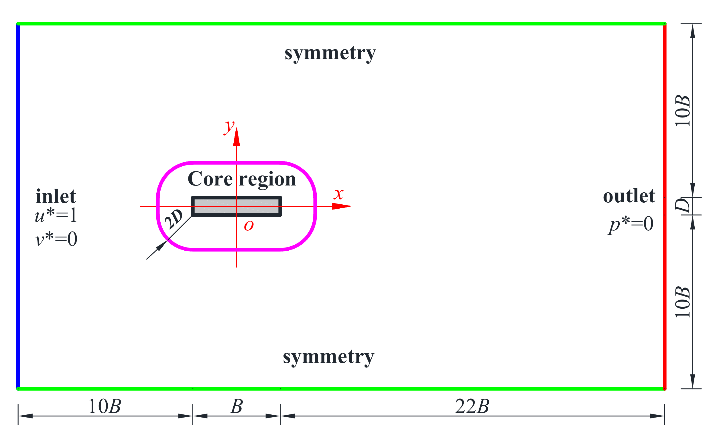
2.2. Computational Domain and Boundary Conditions

The computational domain size for all cases is identical, as is shown in Figure 1, and its dimension is specified based on the best practice recommendations for the BARC project by Bruno and Salvetti [40]. The geometrical centroid of the cylinder is specified as the origin of the Cartesian coordinate system with its streamwise and transverse dimensions denoted as B and D, respectively. Computational grids are locally refined near the cylinder surface that corresponds to the core region plotted in Figure 1. The inlet boundary condition is specified at 10B from the windward side of the cylinder while the outlet boundary condition is situated at 22B from the leeward side of the cylinder. Both top and bottom boundaries of the domain have distances of 10B from the cylinder surfaces.

A Reynolds number ($\mathit{Re}=U_{\infty }D/\nu$) of 4 × 10⁴ is chosen with $U_{\infty }$, D, and ν being the free stream velocity, cylinder width, and kinematic viscosity of the fluid, respectively. The inlet is specified as a uniform flow with $U_x=U_{\infty }$ and $U_y=0$. At the outlet, the convective boundary condition is specified for the velocity, whereas the pressure is set as zero. The top and bottom boundaries are set as symmetry planes. On the surface of the rectangular cylinder, a no-slip boundary condition with zero normal pressure gradient is specified.

With the condition of AoA = 45° chosen as an example, the grid distribution near the cylinder is plotted in Figure 2. Identical grid distribution is specified at the core region for different AoAs. The grid is coarsened from the core region toward the far field regions with an expansion ratio below 1.02. The grid independency study is carried out by performing simulations on grids with three resolutions named Coarse, Medium, and Fine grids, with corresponding cell amounts of 583,280, 984,910, and 1,182,960, respectively. Their near-wall grid heights are δ/D = 4 × 10⁻³, 2 × 10⁻³, and 1 × 10⁻³, which results in distances in wall units (y+)_max being 2, 1, and 0.65, respectively. The non-dimensional time steps defined using $t^{*}=\Delta t{U}_{\infty }/D$ are specified as 1 × 10⁻³, 6 × 10⁻⁴, and 3 × 10⁻⁴ to control the maximum Courant-Friedrichs-Lewy (CFL) numbers being less than 0.5. In each simulation, results from the first 200 non-dimensional time units are discarded, after which the flow becomes fully developed and the data from the following 800 time units is collected for analysis. The other parameters for numerical simulations are summarized in

Table 1. The characteristics of computational grids for different cases.

Cases	Cells Number (105)		δ/D (10−3)	Δt* (10−4)	y+	Wall Nodes
	Core Region	Total
0°-Coarse	245,100	583,280	4	10	~2	1840
0°-Medium	347,300	984,910	2	6	~1	2080
0°-Fine	425,800	1,182,960	1	3	~0.65	2280
5°	347,300	984,830	2	6	~1	2080
10°, 15°, 20°	347,300	983,180 *	2	5	~1	2080
30°, 45°	347,300	982,050 *	2	4	~1	2080

* The total number of cells varies slightly with different AoAs, and the difference is less than 3000.

.

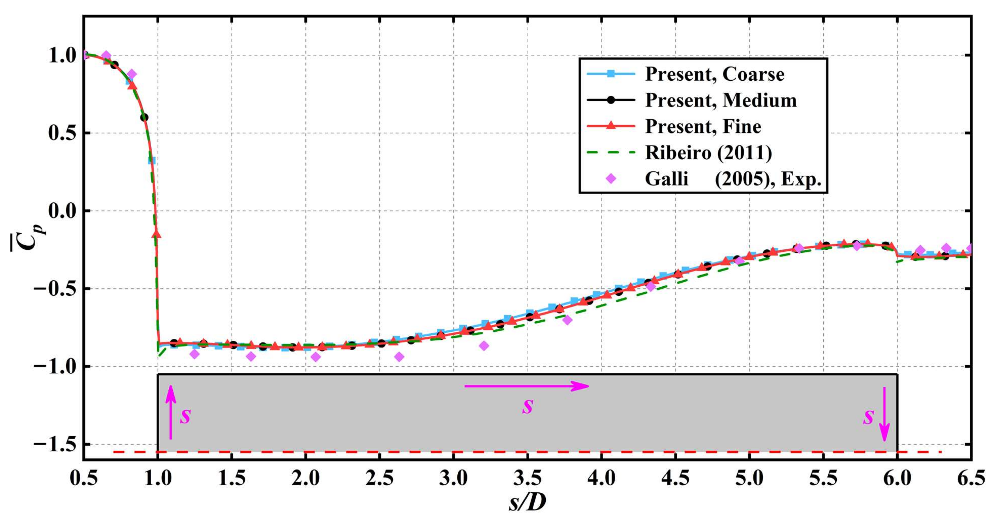
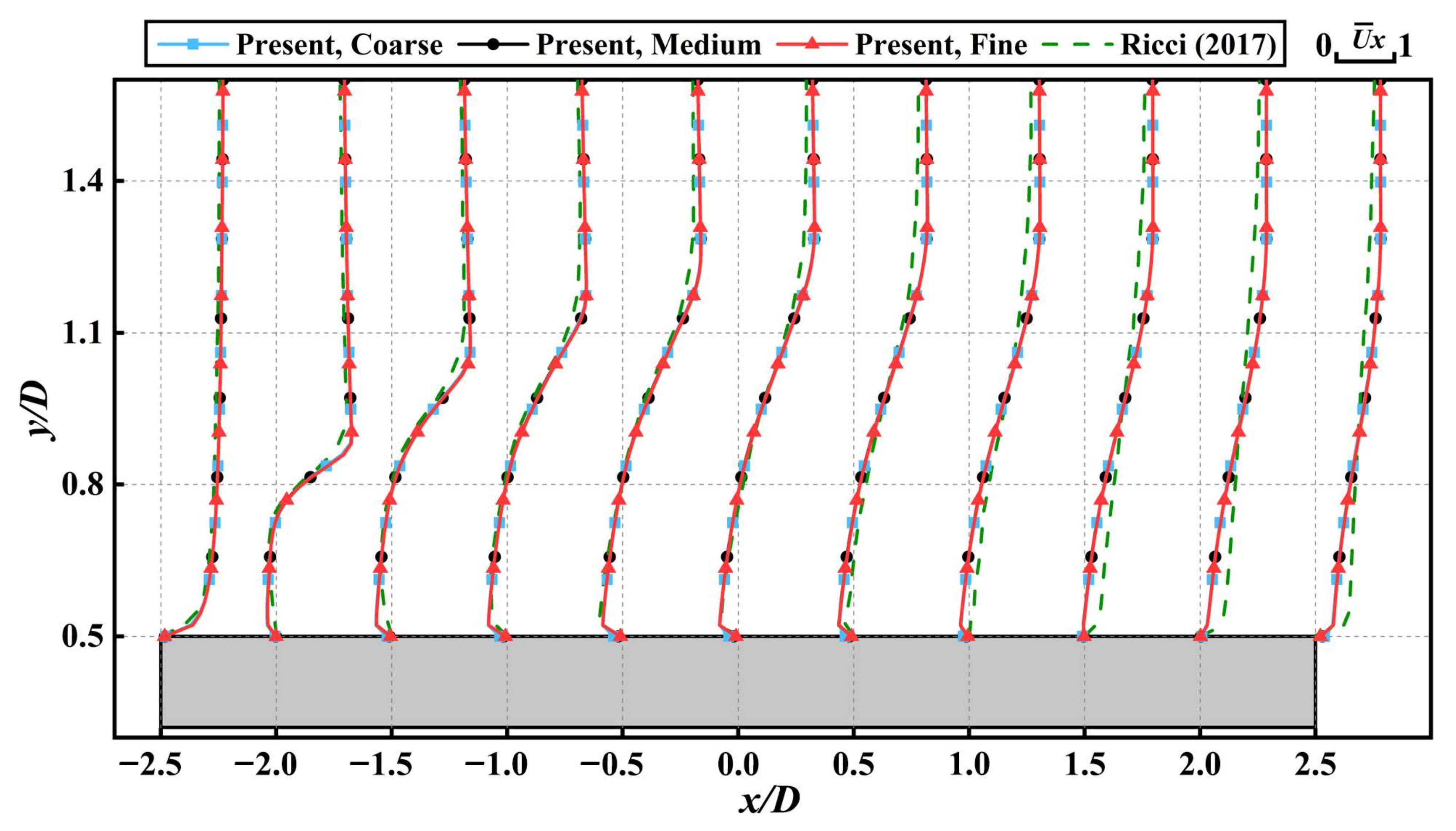
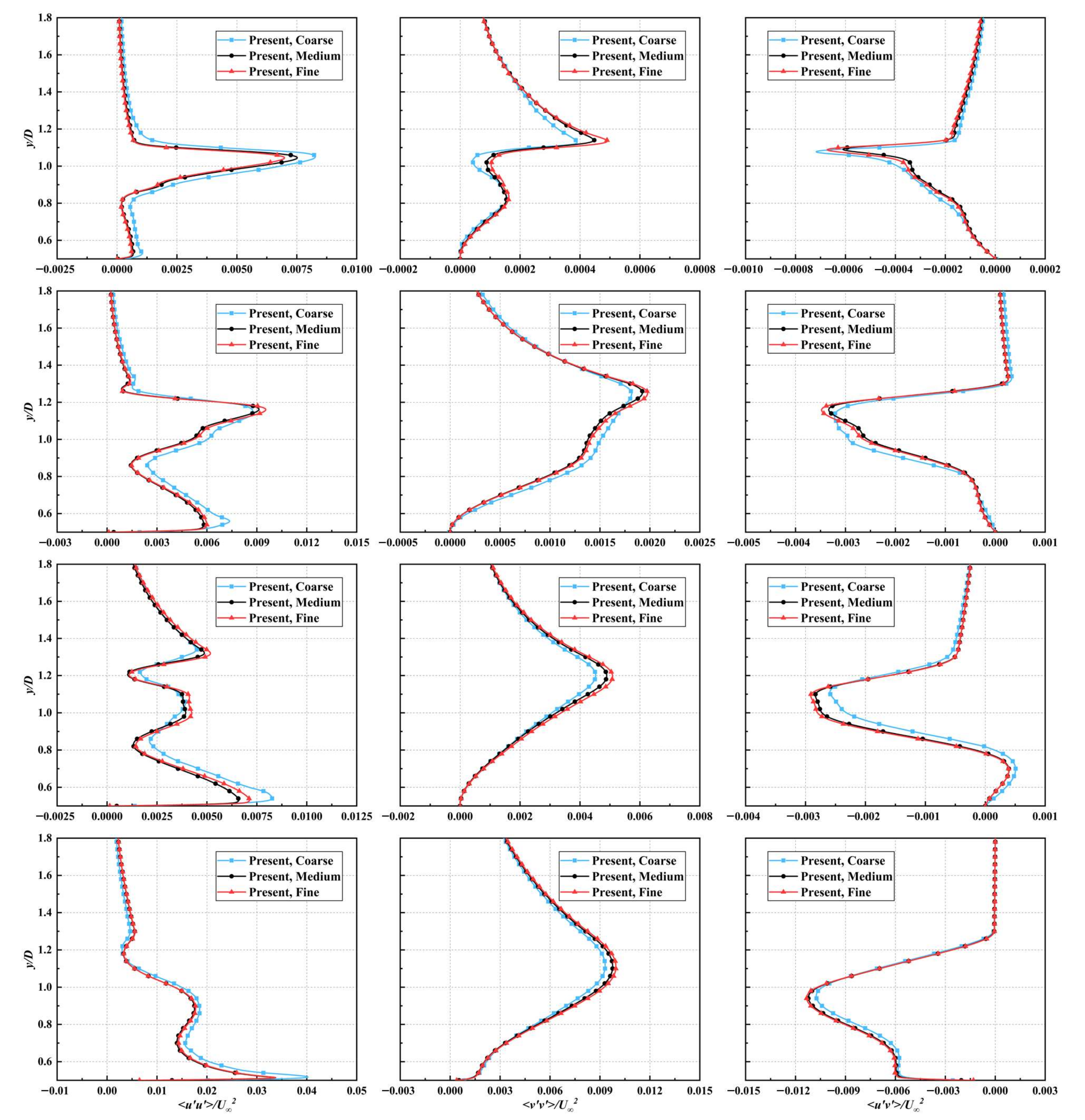
2.3. Numerical Validation

To validate the current numerical model, the 5:1 cylinder at α = 0°, Re = 40,000 is chosen, and both hydrodynamic forces and flow characteristics derived from this study are compared with the experimental results of Galli [41], the 2D URANS simulation results of Ribeiro [42], and the 3D LES simulation results of Bruno et al. [2], Grozescu et al. [43,44], and Ricci et al. [6].

Validation of lift coefficient, drag coefficient, and Strouhal number is initially carried out with their definitions being:

$$C_l=\frac{F_l}{\frac{1}{2}\rho U_{\infty }^{2}D},\dots C_d=\frac{F_d}{\frac{1}{2}\rho U_{\infty }^{2}D},\dots St=\frac{f_{st}D}{U_{\infty }}$$

(12)

where F_d and F_l are the x- and y-directional components of the total hydrodynamic force. The cylinder width D is taken as the characteristic length, and f_st is the vortex shedding frequency, which is obtained by performing the Fast Fourier Transform (FFT) for the time history of the lift coefficient $C_l$.

Table 2. Comparison of lift and drag coefficient and Strouhal number.

Cases	${\overline{\mathit{C}}}_{\mathit{l}}$	${\mathit{C}}_{\mathit{l}}^{\prime }$	${\overline{\mathit{C}}}_{\mathit{d}}$	St
α = 0°-Coarse	−0.01	0.825	1.146	0.123
α = 0°-Medium	−0.006	0.827	1.145	0.122
α = 0°-Fine	−0.006	0.821	1.143	0.121
Bruno et al. [2]	−0.21	/	0.98	0.12
Ribeiro et al. [42]	/	0.9	1.17	/

lists the comparison of time-averaged lift ${\overline{C}}_l$ and drag coefficient ${\overline{C}}_d$, root mean square (RMS) of lift coefficient $C_l^{\prime }$, and St to the numerical results of Bruno et al. [2] and Ribeiro et al. [42]. Negligible magnitudes of ${\overline{C}}_l$ compared with ${\overline{C}}_d$ indicate statistical convergence with respect to the time of current simulations. It can be concluded from Table 2 that the predicted values of $C_l^{\prime }$, ${\overline{C}}_d$, and St in the present study are very close to the previous results. Comparing the results from different grid resolutions, the minor difference among them indicates sufficient resolution even for the coarsest grid.

Detailed validation is also carried out by comparing the pressure coefficient along the surface of the cylinder, which is calculated using:

$${\overline{C}}_p=\frac{\overline{p}-p_{\infty }}{\frac{1}{2}\rho U_{\infty }^2}$$

(13)

where $\overline{p}$ is time-averaged pressure, $p_{\infty }$ is far-field pressure, and $U_{\infty }$ is free incoming flow velocity. Comparison of ${\overline{C}}_p$ along the top side of the cylinder derived from this work to the numerical results from Ribeiro et al. [42], and the experimental results of Galli [41] are presented in Figure 3. It can be observed that the overall trend of ${\overline{C}}_p$ on the wall of the cylinder is well captured by current simulations, except for the slight overestimation that exists near the leading edge of the cylinder compared to the experimental result of Galli [41]. As the mesh becomes finer, the ${\overline{C}}_p$ gradually approaches the literature results, and the ${\overline{C}}_p$ distributions of Medium and Fine grids almost coincide.

Figure 4 presents the time-averaged streamwise velocity distribution $\overline{U_x}$ around the cylinder. The main recirculation bubble near the side surface of the cylinder is formed due to the separation of the flow from the leading edge of the cylinder. The coordinates of its centroid are denoted as (Xc, Yc). Further, the x-coordinates of the reattachment point and the saddle point are also recorded and denoted as Xr and Xs. A comparison of the locations of these characteristic points with the LES results of Grozescu et al. [43,44] is listed in

Table 3. Coordinate values of feature points of the recirculation bubble.

Case	Xc	Yc	Xr	Xs
α = 0°-Coarse	−0.68	0.81	1.71	3.24
α = 0°-Medium	−0.65	0.81	1.69	3.24
α = 0°-Fine	−0.63	0.80	1.69	3.24
Grozescu et al. [43,44]	−0.88	0.78	1.63	3.3

. The results of Yc, Xr, and Xs exhibit satisfactory accuracy, whereas the x-directional location of the main recirculation bubble derived in current simulations appeared to be closer to the leeward side of the cylinder as the derived Xc is higher than Grozescu et al. [43,44].

To further validate the simulated flow field, fluid velocity distribution derived from LES simulations conducted at Re = 5.5 × 10⁴ by Ricci et al. [6] is compared with present results (Re = 4 × 10⁴) as plotted in Figure 5. Good agreement of the velocity profiles between the results from Ricci et al. [6] and the current simulation demonstrates that the current numerical model has the capability of accurately capturing the development of the flow.

Though the above-mentioned discussion implies that only minor deviation of the results derived from different grid resolutions exists, a comparison of the Reynolds stress profiles demonstrates the necessity of implementing a properly refined mesh. The time-averaged Reynolds stress profiles at x/D = −1.25, 0, 1.25, and 2.5 in the shear layer of the cylinder derived from the three grids are presented in Figure 6. Taking the results from the Fine grid as a reference, the apparent deviation can be seen from the Coarse grid, whereas the Reynolds stress profiles derived from the Medium grid almost coincide exactly with that derived from the Fine grid. As a result, considering both computational efficiency and numerical accuracy, the Medium grid is selected to resolve the flow field around the rectangular cylinder.

3. Results and Discussion

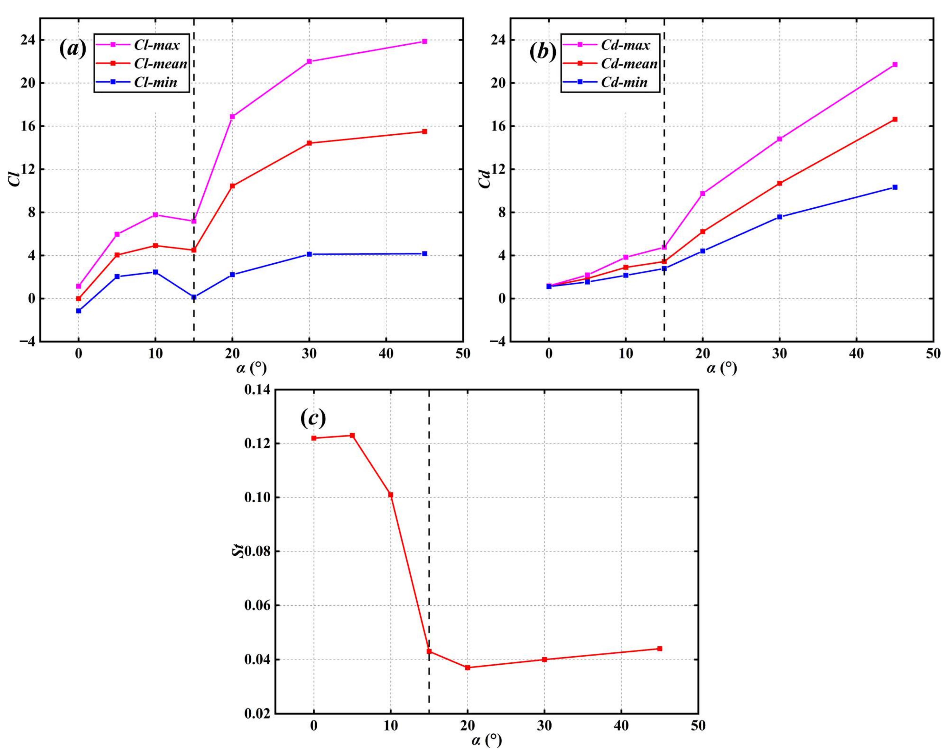
3.1. Force Coefficients Characteristics

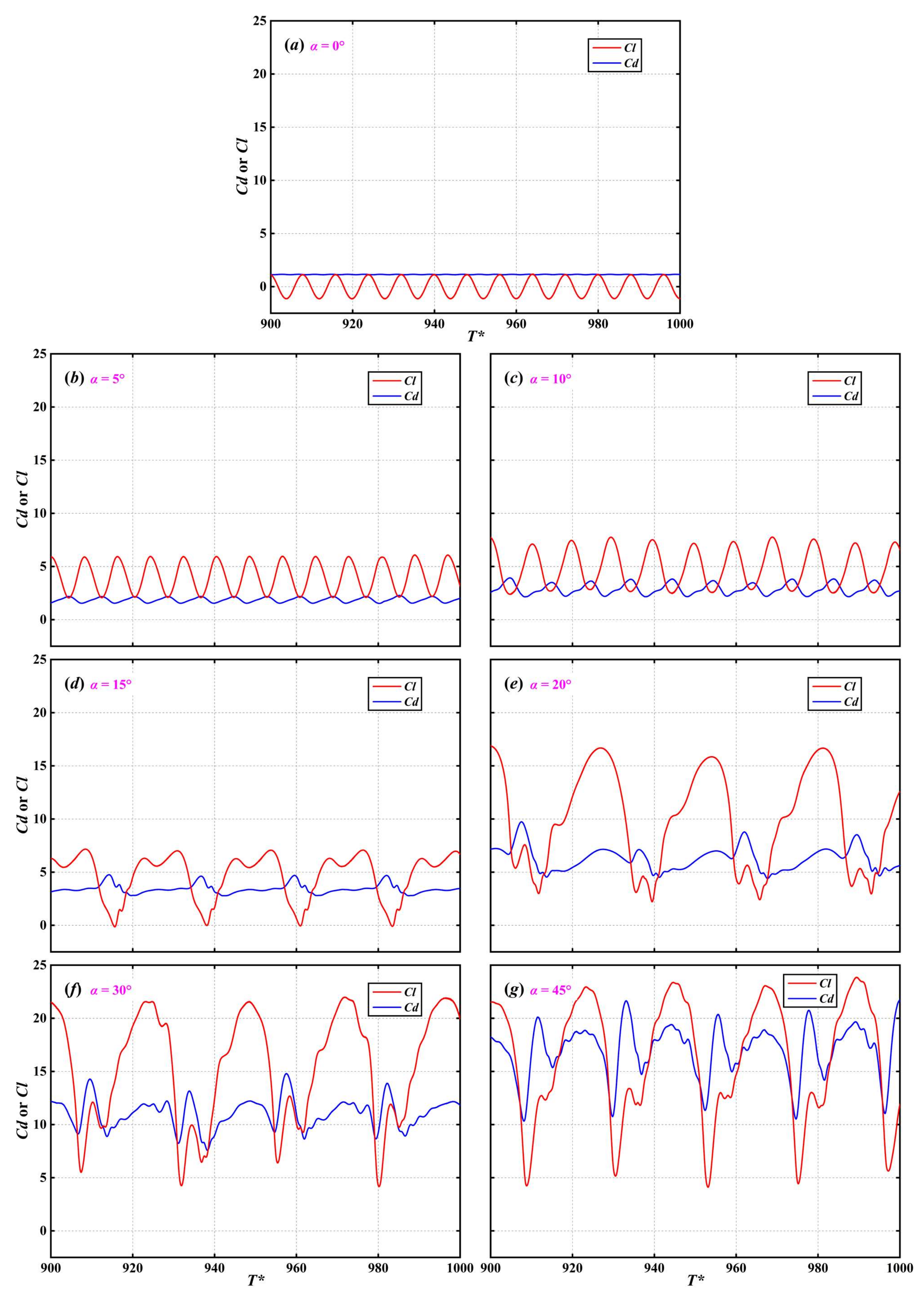
3.1.1. Time Histories of Force Coefficient

The lift coefficient $C_l$ and drag coefficient $C_d$ were studied first, and their temporal developments are plotted in Figure 7. It can be observed that among all AoAs investigated, the fluctuation amplitude of $C_l$ and $C_d$ increased gradually, which indicates that the flow field around the cylinder gradually became more disordered. In more detail, within α = 0°~10°, the $C_l$ and $C_d$ maintain a quasi-sinusoidal trend with small amplitudes. When α ≥ 15°, the amplitude of $C_l$ and $C_d$ increases rapidly, and their fluctuation frequency decreases. Furthermore, the Root Mean Square (RMS) of $C_l$ is always higher than ; that is, the fluctuation amplitude of $C_l$ is greater than that of $C_d$.

The time-averaged lift coefficient ${\overline{C}}_l$ and drag coefficient ${\overline{C}}_d$, together with St at different AoAs, are plotted in Figure 8. The ${\overline{C}}_l$ presents an overall increasing trend with respect to AoA except for the data at α from 10° to 15°, which decrease slightly, whereas the ${\overline{C}}_d$ increases approximately linearly with two distinctive slopes at AoA less and higher than 15°. The St remains almost constant at α ≤ 5° and α ≥ 15° with magnitudes of 0.12 and 0.04, respectively, whereas at 5° ≤ α ≤ 15°, an abrupt drop in the St exists. In summary, at α = 0°~10°, similar characteristics of the force coefficient can be observed. At α = 15°, the flow is transitional. When α = 20°~45°, a different pattern of force coefficient characteristics appears. This will be further discussed in Section 3.2.1.

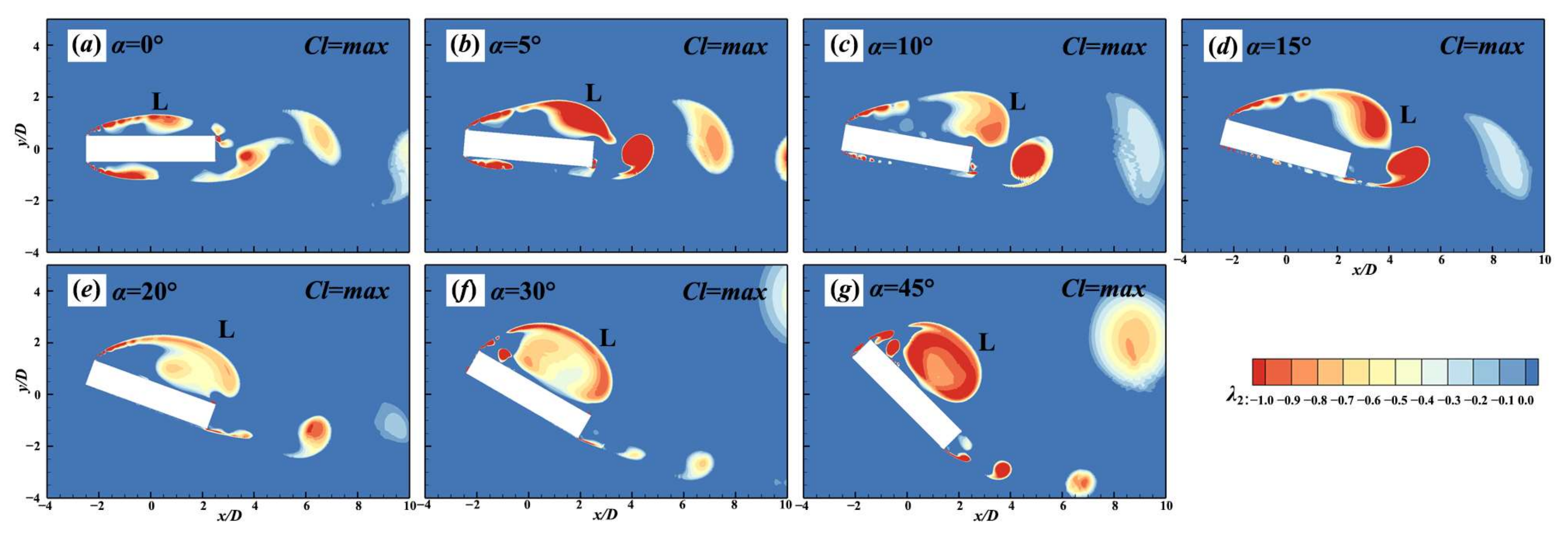
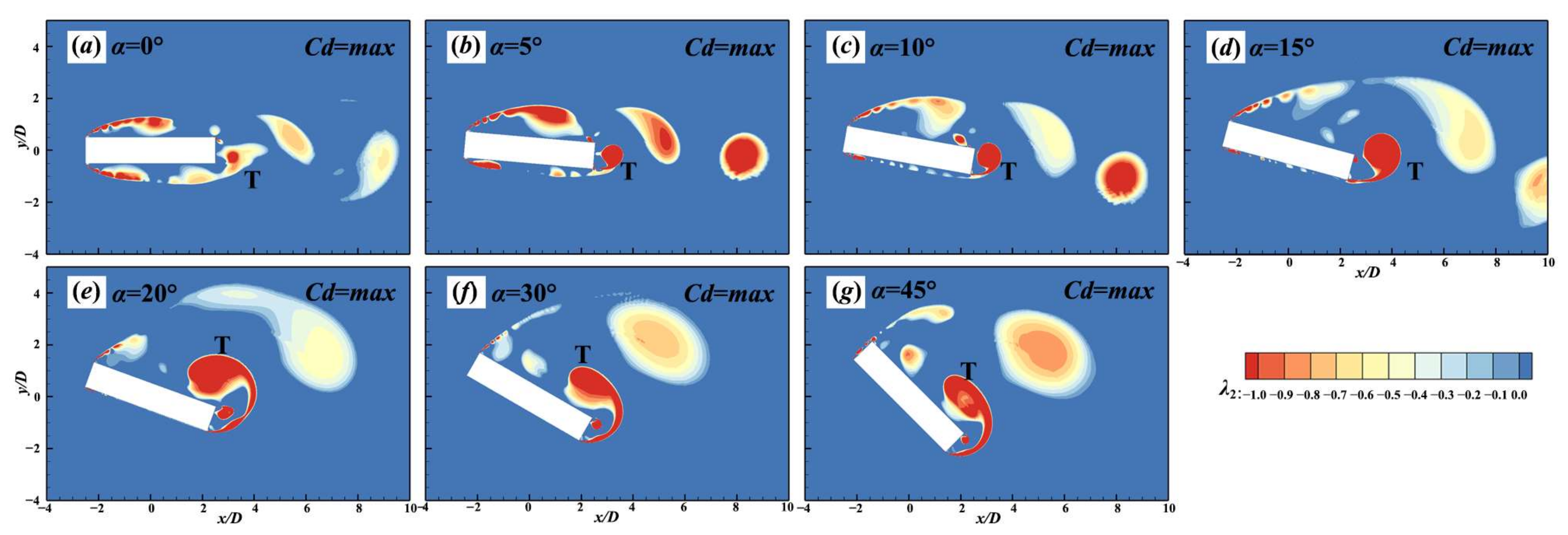
3.1.2. Relationships between Force Coefficients and Vortex Structure

In this paper, the λ₂ criterion [45] based on the local velocity gradient tensor $\nabla V$, namely the vortex strength criterion, is used to identify the vortex structure in the flow. The velocity gradient tensor is composed of a symmetric part (strain rate tensor) and an antisymmetric part (rotation rate tensor).

$$\nabla V=\frac{1}{2}(\nabla V+\nabla V^T)+\frac{1}{2}(\nabla V-\nabla V^T)=S+\Omega$$

(14)

where $\nabla V$ means the velocity gradient tensor, $S$ means the strain rate tensor and $\Omega$ means the rotation rate tensor.

If the three eigenvalues of $S^2+{\Omega }^2$ have the following relationship

$${\lambda }_1>{\lambda }_2>{\lambda }_3$$

(15)

then the vortex is identified when the second largest eigenvalue ${\lambda }_2<0$ appears.

As intensive fluctuation in the forces applied by the flow can lead to failures of the submerged engineering structures, a detailed investigation of the flow field is necessary. The instantaneous vortex structure when lift and drag coefficients reach their maximum at different AoAs is plotted in Figure 9 and Figure 10, respectively. It can be seen from Figure 9 that when the lift coefficient reaches its maximum, the downstream traveling vortex shed from the top corner of the leading edge (L-vortex) reaches the top surface of the cylinder, implying its primary influence on the lift force. Furthermore, its location has a trend of moving downstream at AoA increases from 0° to 15°, especially as α = 15° when the core region of the L-vortex leaves almost completely from the top surface, which may be the cause of the drop in the maximum lift coefficient between AoAs at 10° and 15°, as is plotted in Figure 8a. When the AoA increases from 15° to 45°, an upstream trend of moving can be observed. Turning the focus onto the flow field when drag reaches maxima, as is plotted in Figure 10, the commonality for different AoAs is that the vortex shed from the bottom corner of the trailing edge (T-vortex) reattaches to the cylinder. At α ≤ 15°, the effect of such recirculation flow is mainly experienced by the leeward side of the cylinder. When α > 15°, the T-vortex moves to the top surface of the cylinder, which has a much larger area than the leeward side of the cylinder. The increase in the plane of action may be the cause of the steeper slope in the maximum drag at α > 15°, as illustrated in Figure 8b.

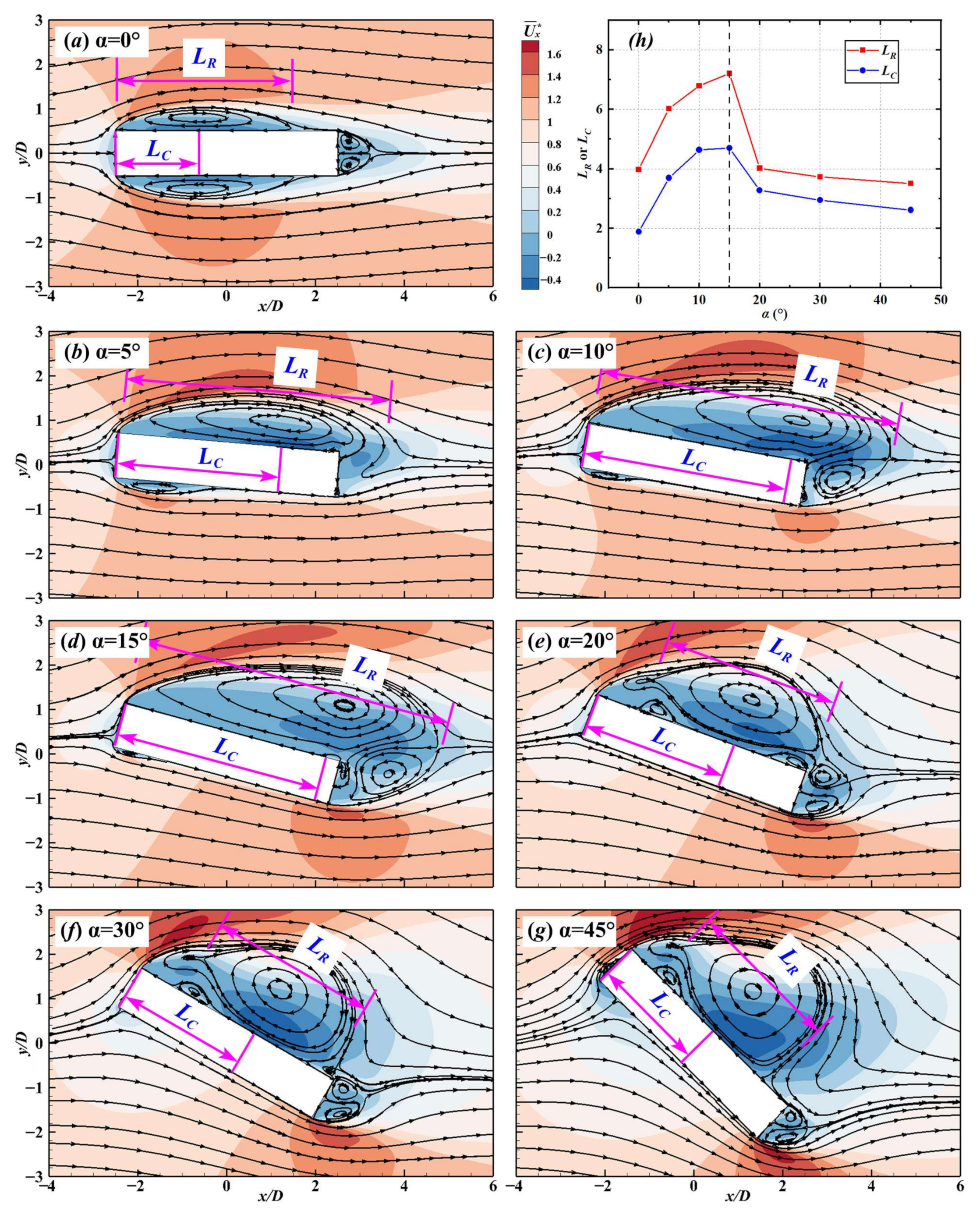
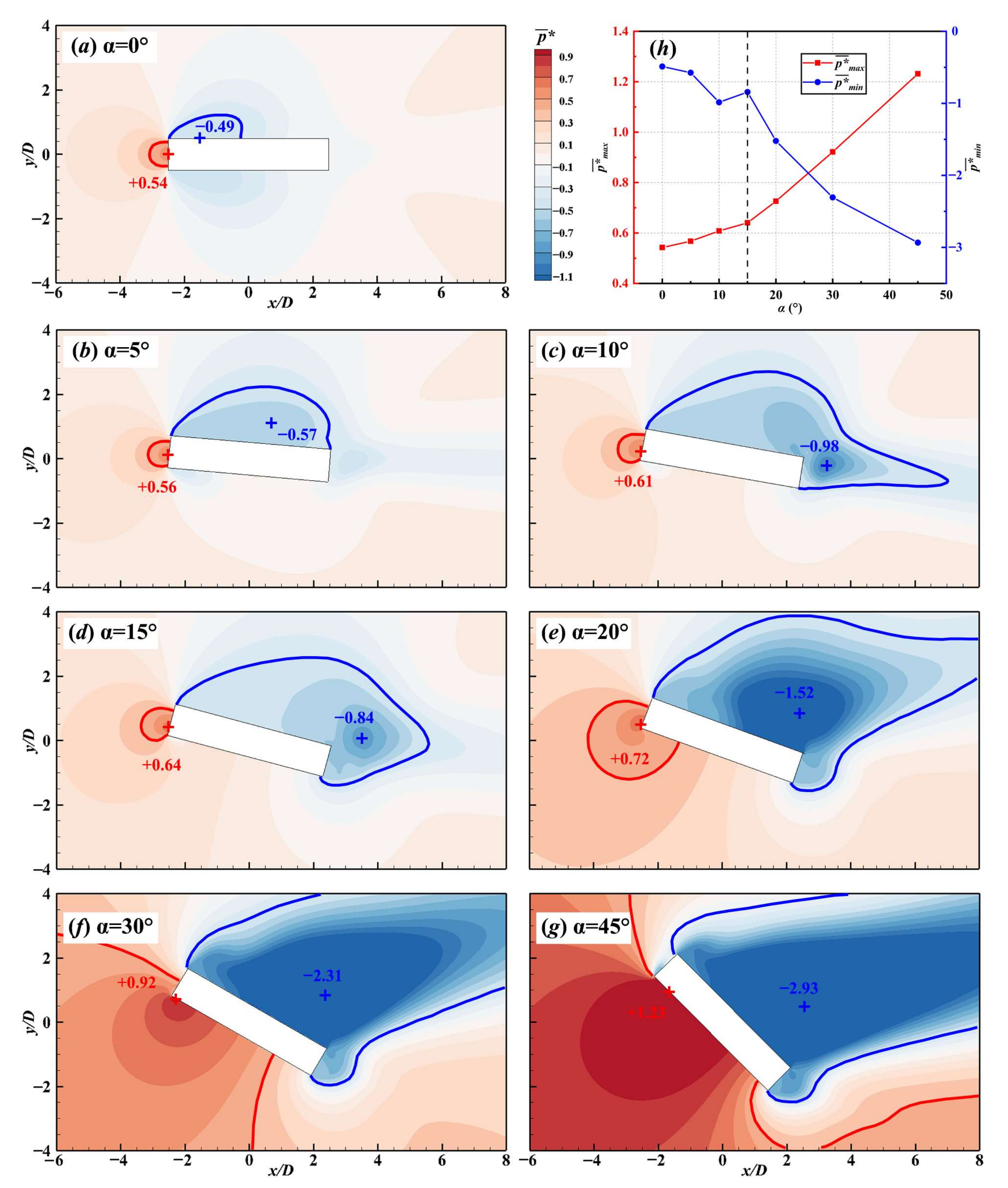
3.2. Effects of AoA on Global Flow Characteristics

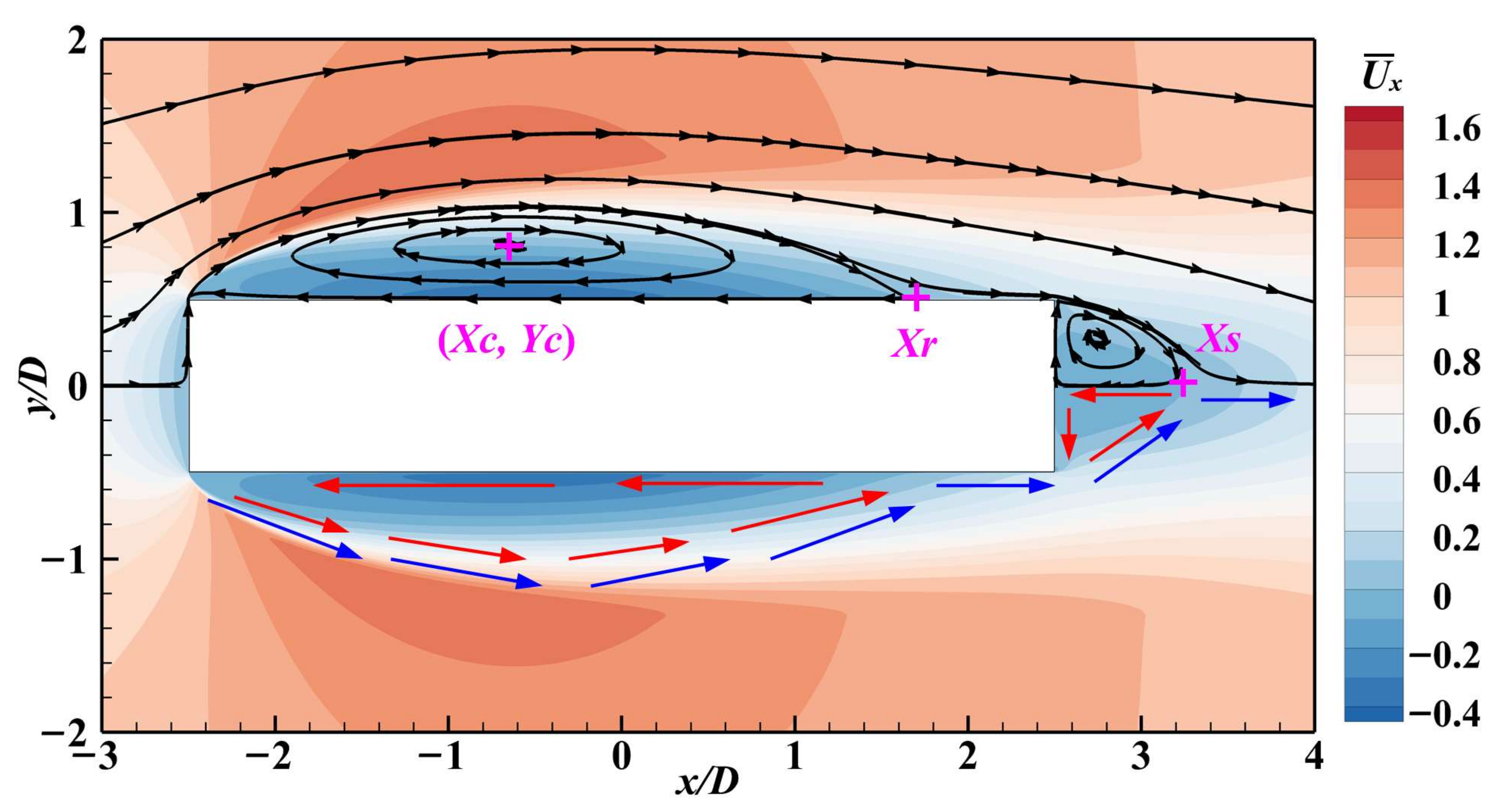
3.2.1. Time-Averaged Separation and Reattachment

Figure 11 shows the time-averaged streamwise velocity contours together with the streamline under different AoAs. The main recirculation bubble on the top side of the cylinder changes greatly with the AoA. L_R denotes the x′-length of the main recirculation bubble on the top side, while L_C represents the x′-directional distance from the center of the main recirculation bubble to the leading edge of the rectangular cylinder. It can be concluded from Figure 11h that both L_R and L_C show the same trend, increasing at first and reaching the maximum at α = 15°, then decreasing with the increase in the AoA. This turning point, designated by a black dashed line, also appears in the lift coefficient and drag coefficient diagrams, as shown in Figure 8. The position of recirculation bubbles is also a negative pressure zone, which has a significant impact on lift and drag force.

As the AoA increases from 0° to 15°, as shown in Figure 11a–d, the flow separates at the two corners of the leading edge with an increased recirculation bubble length on the top side and a decreased bubble length on the bottom side. This variation in the upper and lower recirculation bubbles all can improve the lift force. However, when α = 15°, the center of the main recirculation bubble deviates from the trailing edge of the cylinder resulting in a slight decrease in lift. Further, the summation of the lengths of these two recirculation bubbles remains almost constant with a magnitude approximately equal to twice the x-length of the main recirculation bubble at α = 0°, which is consistent with the observation from Wu et al. [8]. As the AoA increases to 20°~45°, as plotted in Figure 11e–g, the bottom side of the cylinder becomes the upstream surface, resulting in the diminishment of the recirculating flow around it. Meanwhile, the extension of the recirculation bubble on the top side of the cylinder gradually shrinks, and a small recirculation bubble arises beneath the main recirculation bubble.

In addition, there also exists a pattern of development in the wake recirculation bubbles behind the leeward side of the cylinder at α > 0°. At α = 5°, the recirculation bubble does not exist in the wake. When the AoA increases to 10°~15°, a large wake recirculation bubble is formed, which is about 3 times as long as that of α = 0°. When the AoA is further increased to 20°~45°, the number of wake recirculation bubbles is increased to 2. The wake recirculation bubbles played a role in increasing the drag force. At the same time, as the AoA increases, the main recirculation bubble gradually transfers to the rear side of the cylinder, which also leads to a large increase in drag force.

3.2.2. Pressure Distribution in the Flow Field

The time-averaged pressure at different AoAs is also calculated and plotted in Figure 12. The blue and red lines represent the locations with $\overline{p}*(=\overline{p}/\rho U_{\infty }^2)$ values of −0.4 and 0.4, respectively. The numbers in the figure indicate the maximum and minimum value of pressure with the symbol “+” marking their location. It can be seen from Figure 12h that with the increase in the AoA, the variation in the maximum and minimum pressure in the flow field follows a characteristic similar to that of the lift and drag coefficient. More specifically, aside from the overall tendency to decrease, the P_min increases at an AoA between 10° and 15°, and this might be correlated with the decrease in the lift coefficient between these two AoAs in Figure 8a. On the other hand, a continuous increase in P_max can be observed with its slope steeper at α > 15° compared to the results at α < 15°, which is similar to the variation in drag coefficient in Figure 8b. As the AoA increases, larger low-pressure and high-pressure regions are formed near the top and bottom sides of the cylinder, respectively. Except in the range of α = 0°~15°, the high-pressure region near the windward side of the cylinder basically remains invariant.

3.3. Effects of AoA on Local Flow Characteristics

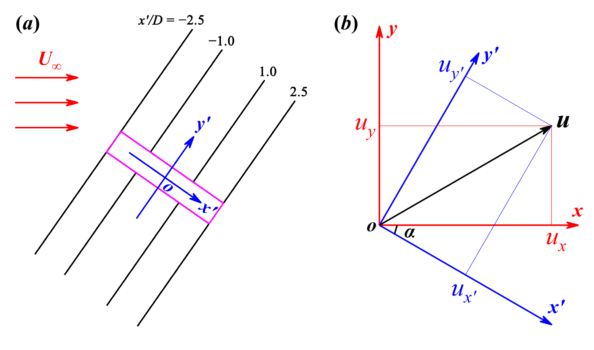
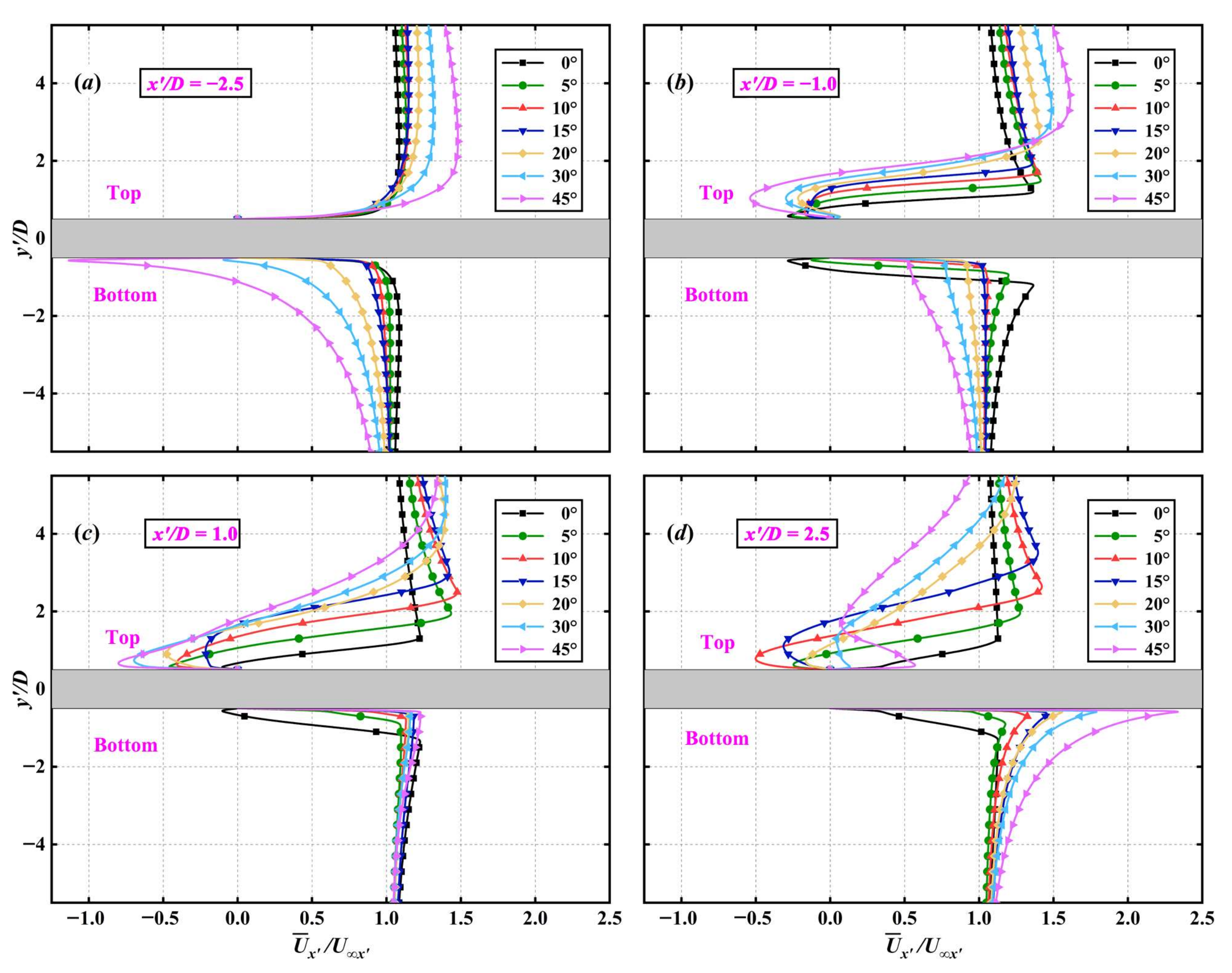
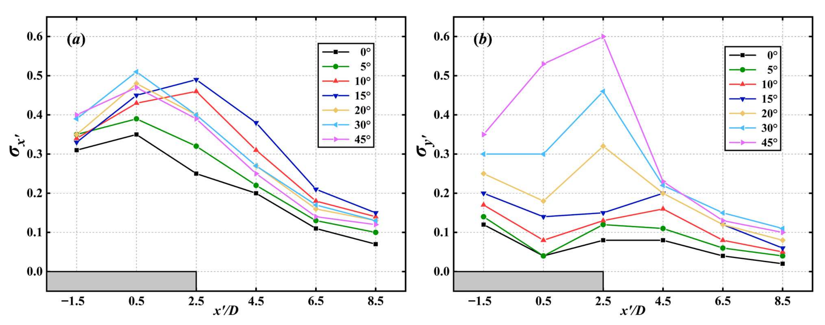
3.3.1. Mean and Fluctuating Velocity Distribution in the Flow Field

To better understand the velocity distribution around the rectangular cylinder, the fluid velocity was sampled along 4 cross sections that are perpendicular to the top and bottom side of the cylinder with x′/D = −2.5, −1.0, 1.0, 2.5.

Figure 13a shows the arrangement of the cross sections, and Figure 13b demonstrates the relative position of the global coordinate system xoy and the local coordinate system x′oy′ that is obtained by rotating the global coordinate system around the origin for an angle of AoA. Additionally, the flow velocities ($U_{x\prime }$,$U_{y\prime }$) along local x′- and y′-axis are derived from:

$$\left\{\begin{array}{l}{U}_{x\prime }=U_x\cos (\alpha )-U_y\sin (\alpha )\\ U_{y\prime }=U_x\sin (\alpha )+U_y\cos (\alpha )\end{array}\right.$$

(16)

Similarly, the free incoming flow velocity $U_{\infty }$ is decomposed into $U_{\infty x\prime }$ and $U_{\infty y\prime }$ along the x′- and y′-directions, respectively:

$$\left\{\begin{array}{l}{U}_{\infty x\prime }=U_{\infty }\cos (\alpha )\\ U_{\infty y\prime }=U_{\infty }\sin (\alpha )\end{array}\right.$$

(17)

Figure 14 shows the time-averaged x′-directional flow velocity profile ${\overline{U}}_{x\prime }$ along the 4 cross sections for the cylinders at different AoAs. The inflection point of the velocity curve can be approximately considered as the boundary of the shear layer. On the top side of the cylinder, the thickness of the shear layer increases gradually with the increase of the AoA, while on the bottom side of the cylinder, the thickness of the shear layer is very thin. This can be attributed to the fact that as the AoA increases, the top side is gradually transformed into the leeward, and the bottom side becomes windward. In addition, with the increase of AoA, the shear layer boundary is gradually blurred, especially when α > 15°. This may result from the higher turbulence intensity induced in the leeward region as the AoA increases and the strengthening of the momentum exchange in the inner and outer zones of the shear layer. According to the characteristics of ${\overline{U}}_{x\prime }$ distribution at different AoAs, it can be roughly divided into two flow modes (α = 0°~15° and α = 20°~45°), which will be discussed in detail in Section 3.4.

To understand the uniformity of the ${\overline{U}}_{x\prime }$ and ${\overline{U}}_{y\prime }$ distribution around the cylinders at different AoAs, the standard deviation of time-averaged velocity is introduced for analysis. Taking ${\overline{U}}_{x\prime }$ as an example, its standard deviation is calculated using:

$${\sigma }_{x\prime }=\sqrt{\frac{{\displaystyle \sum {({\overline{U}}_{x\prime }-{\overline{U}}_{\infty x\prime })}^2}}{n-1}}$$

(18)

where ${\overline{U}}_{\infty x\prime }$ is the x′-directional component of the far-field flow velocity and n is the number of the sampling points on each section; 1000 is selected for n at sections with x′/D = −1.5, 0.5, and 2.5 (at y′/D = [−5.5, −0.5)∪(0.5, 5.5]) and 1101 is specified at sections x′/D = 4.5, 6.5, and 8.5 (at y′/D = [−5.5, 5.5]). The standard deviation ${\sigma }_{y\prime }$ of ${\overline{U}}_{y\prime }$ is calculated in a similar manner.

Figure 15a,b shows the variation in the standard deviation of time-averaged velocity with respect to the AoA, which is positively correlated with the AoA. The ${\sigma }_{x\prime }$ shows a trend of increasing initially and then decreasing. The uniform incoming flow separates from the leading edge corner, forming a recirculation bubble, resulting in an increased ${\sigma }_{x\prime }$ along the cylinder. As the sampled location deviates from the cylinder, the ${\sigma }_{x\prime }$ decreases. From the perspective of different AoAs, when the AoA increases, the ${\sigma }_{x\prime }$ also increases, except for α = 10° and 15°, which show higher values than other AoAs in the wake region. This may be due to the existence of a large wake bubble behind the trailing edge of the cylinder, as can be seen in Figure 11c,d.

The ${\sigma }_{y\prime }$ in Figure 15b also shows an increasing trend as the AoA increases. Under relatively low AoAs (0~15°), the ${\sigma }_{y\prime }$ fluctuates slightly along the direction of the cylinder, which is stable between 0.05~0.2, and its value is less than ${\sigma }_{x\prime }$, indicating that the degree of dispersion of the ${\overline{U}}_{y\prime }$ is less than that in the ${\overline{U}}_{x\prime }$. However, the ${\sigma }_{y\prime }$ around the cylinder increases significantly at α = 20~45°. As the AoA increases, the blocking effect of the cylinder against the incoming flow signifies, and its influence is more prominent for ${\sigma }_{y\prime }$ than ${\sigma }_{x\prime }$, as can be observed in Figure 11 and Figure 12.

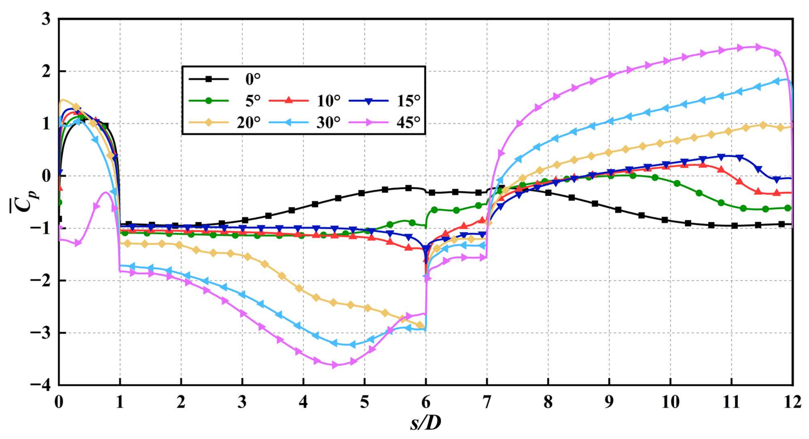
3.3.2. Pressure Coefficient Distribution over the Cylinder Surface

The time-averaged pressure coefficient ${\overline{C}}_p$ around the cylinder under different AoAs is shown in Figure 16. The definition of s/D can be found in Figure 2d. Windward side of the cylinder that corresponds to s/D < 1 always has positive ${\overline{C}}_p$ except for the case with α = 45°, which possesses negative pressure caused by the formation of recirculation flow. On the top side (s/D = 1~6) of the cylinder at α = 0°, a negative pressure ${\overline{C}}_p$ with an approximate magnitude of −1 is generated within the range of 1.7D, which is approximately equal to the distance from the leading-edge corner to the center of the main recirculation bubble (Lc = 1.85D at Figure 11a). At α = 5°~15°, ${\overline{C}}_p$ distribution on the top side remains almost invariant, which can also be seen from Figure 11b–d that the top side of the cylinder is entirely covered by the main recirculation bubble, and the center of the main recirculation bubble is near the trailing edge. When α ≥ 20°, the position with the low-pressure coefficient region also roughly corresponds to the location of the main bubble on the top side of the cylinder, as is plotted in Figure 11e–g. With the increase of the AoA, the pressure coefficient decreases on the leeward side of the cylinder (s/D = 6~7) and then increases gradually on the bottom surface (s/D = 7~12).

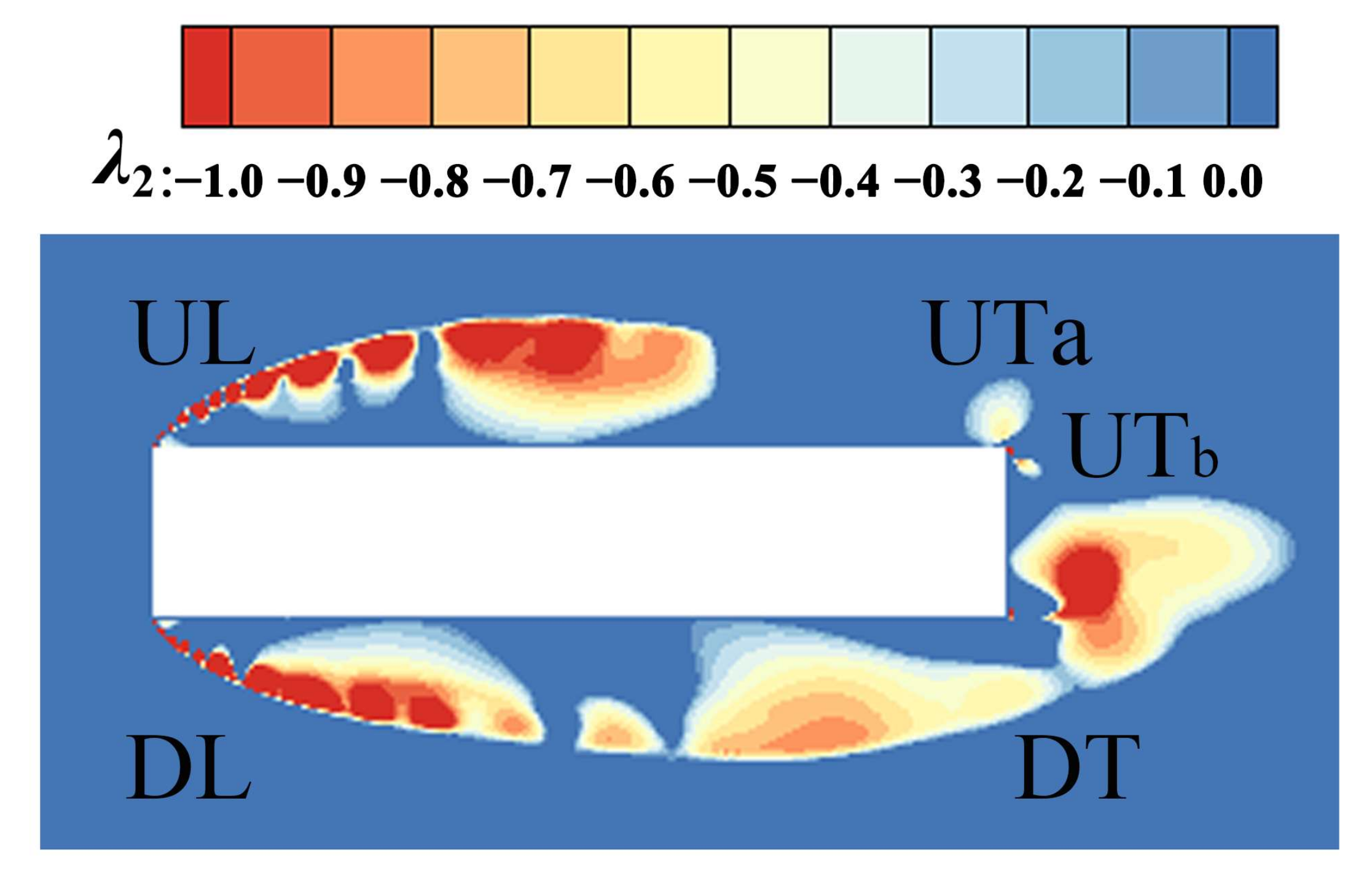
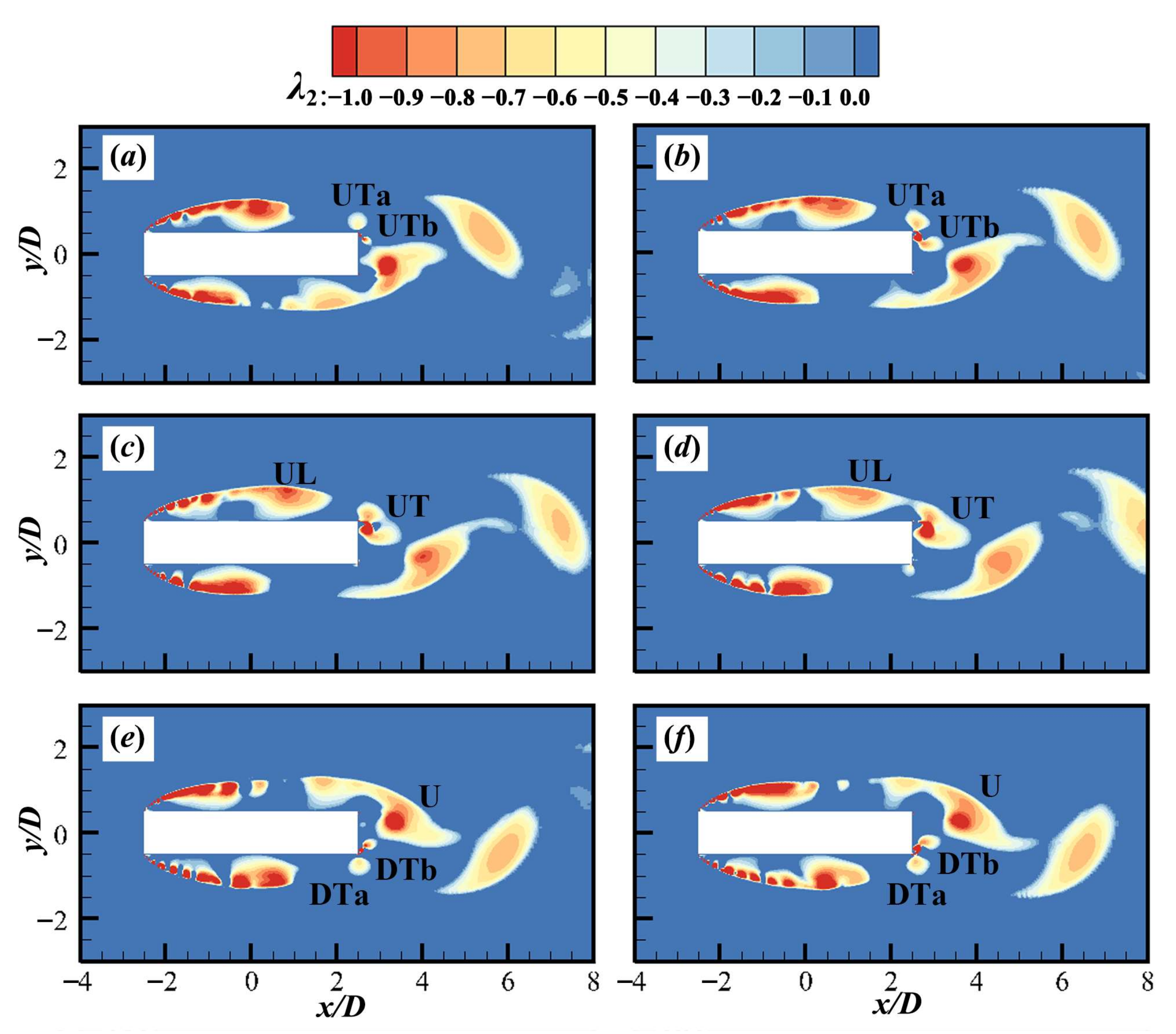
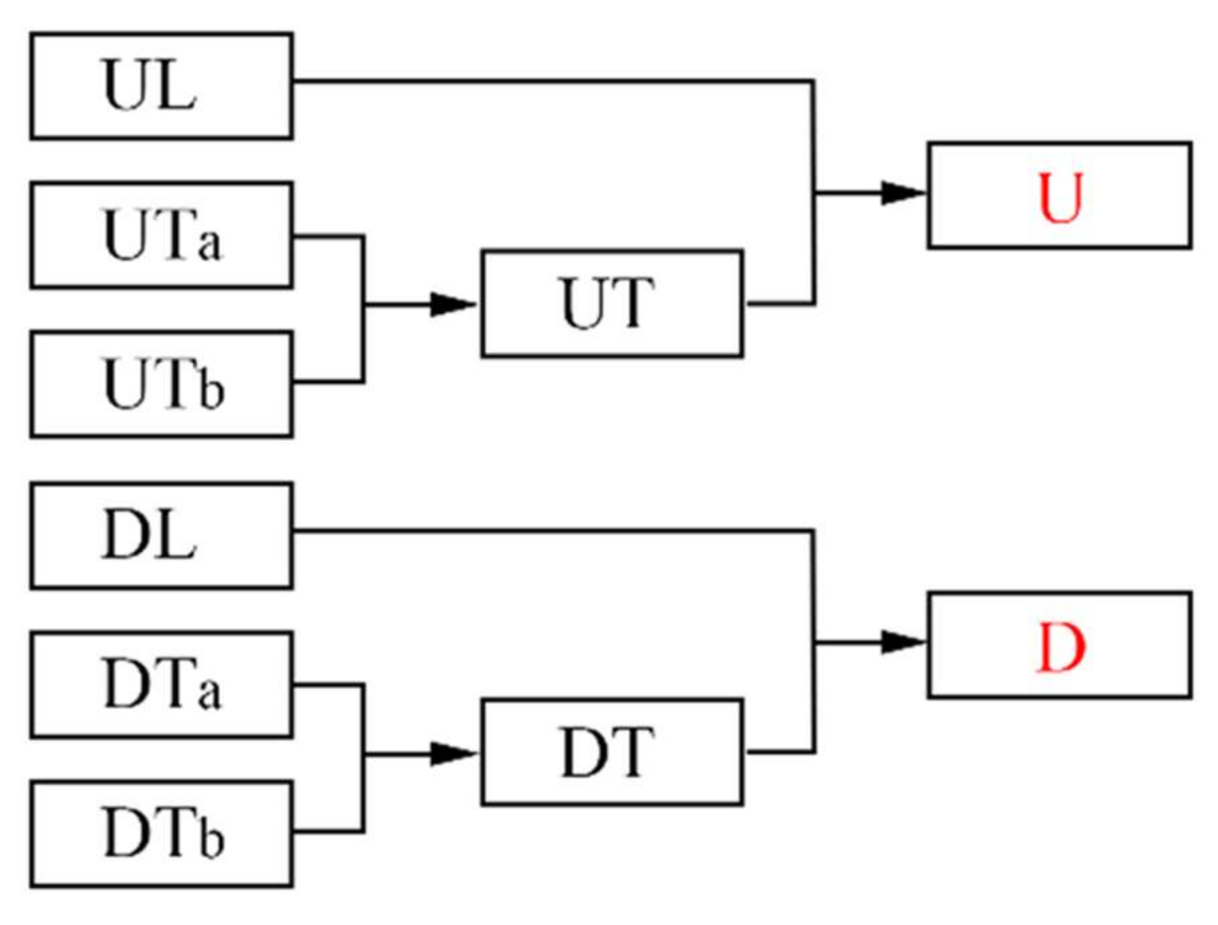
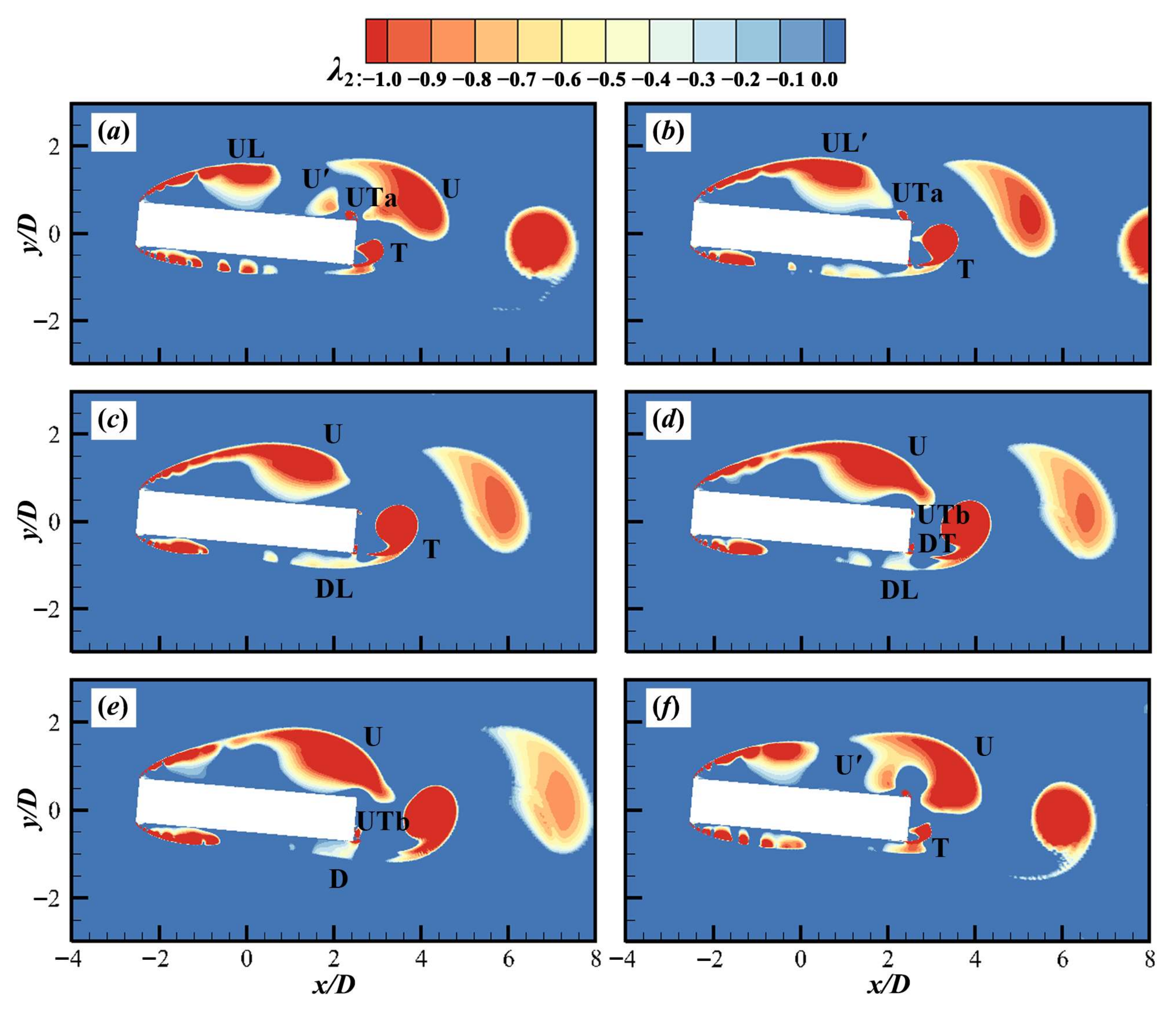
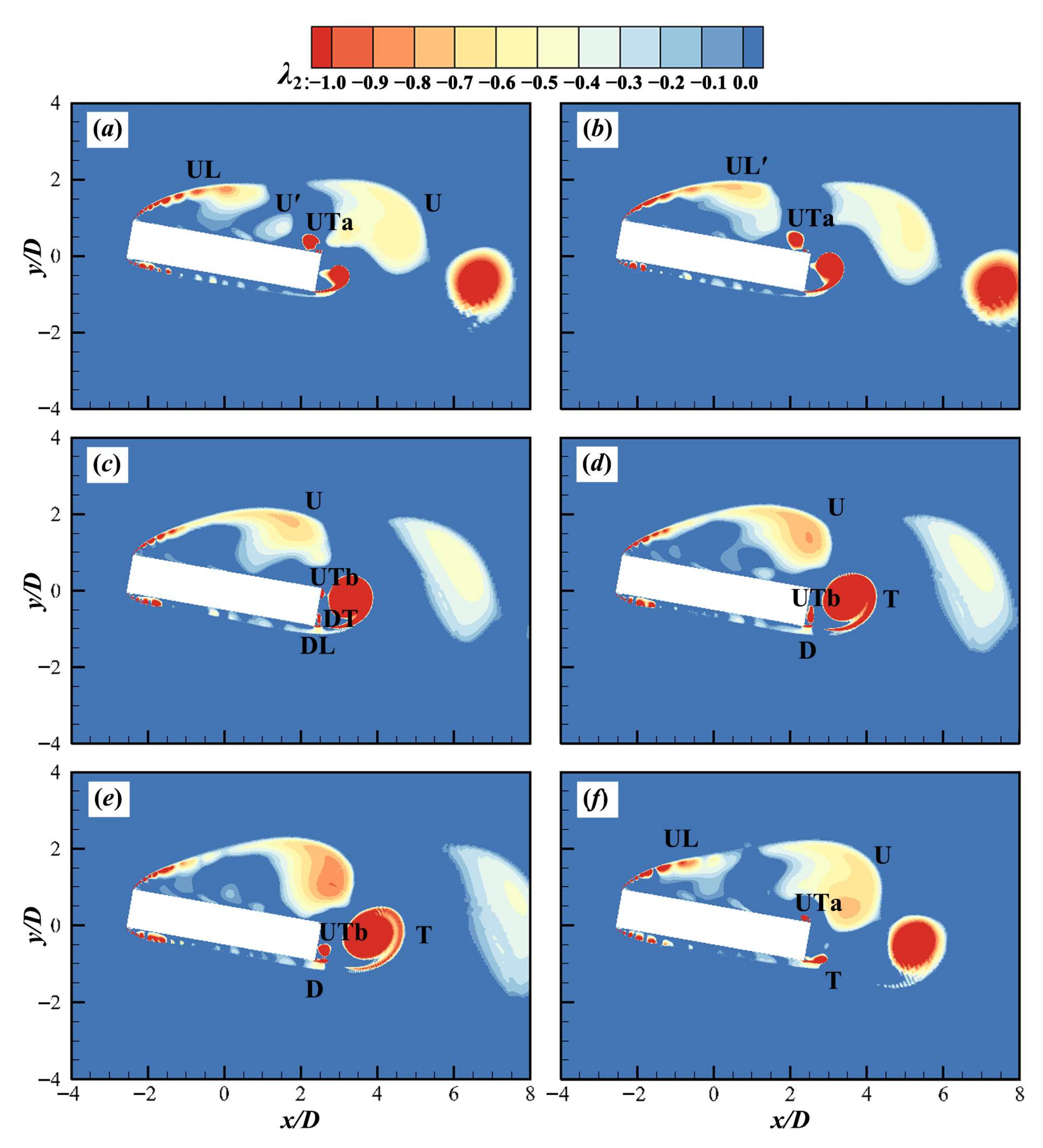
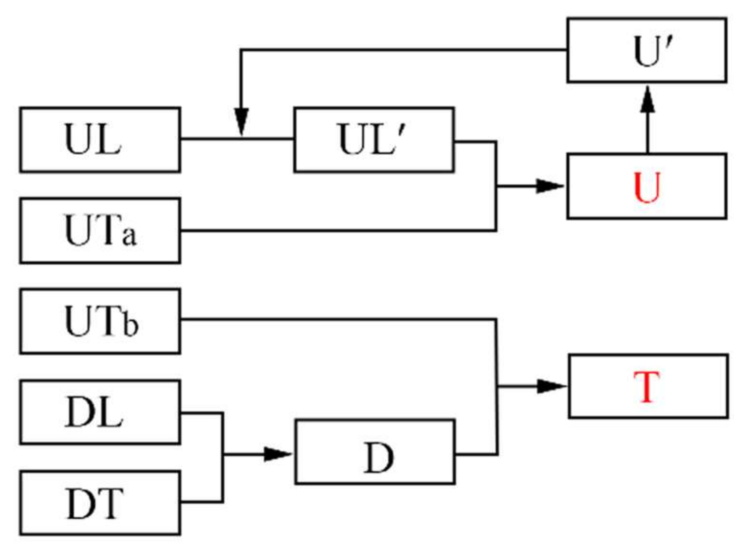
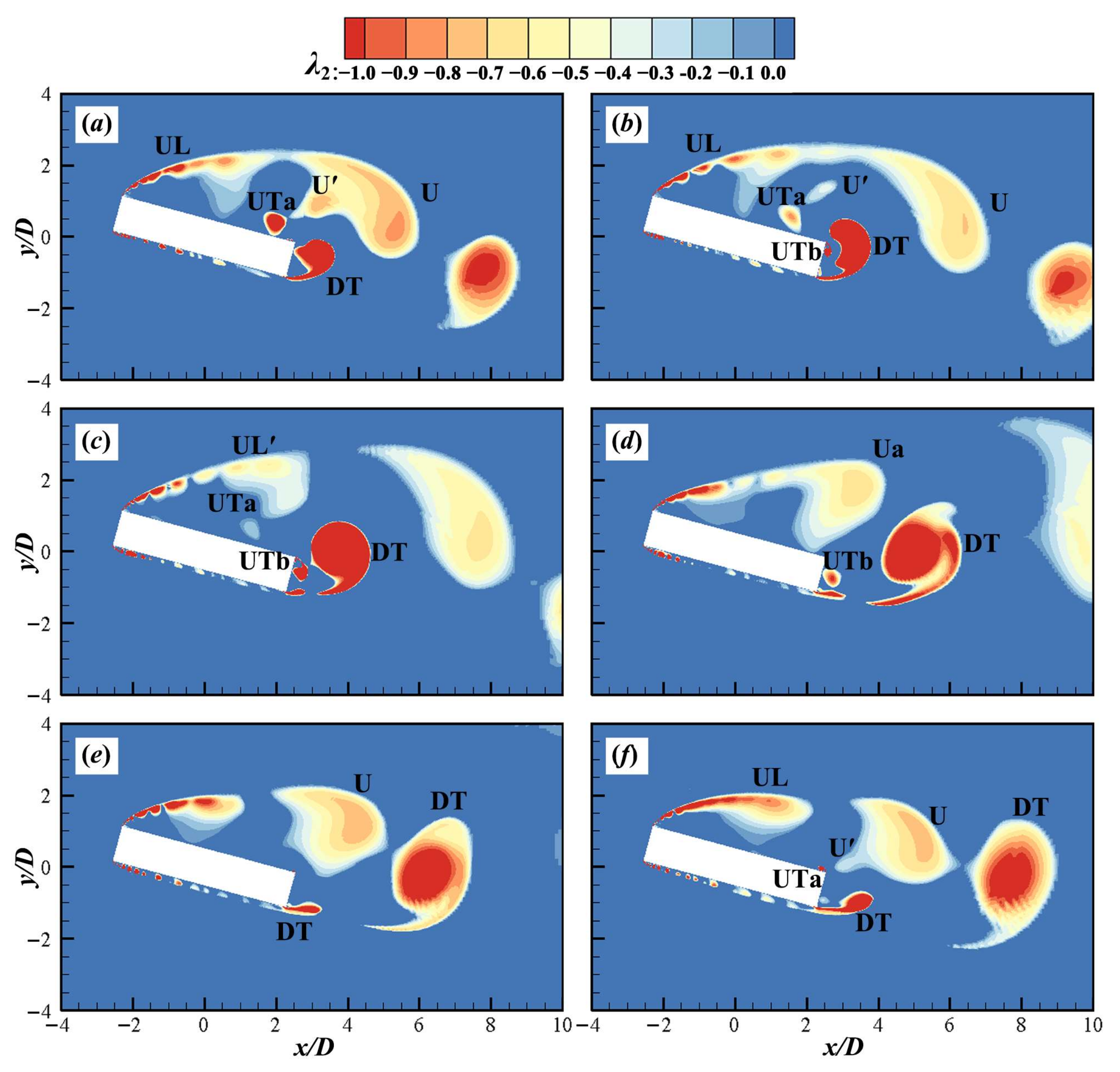
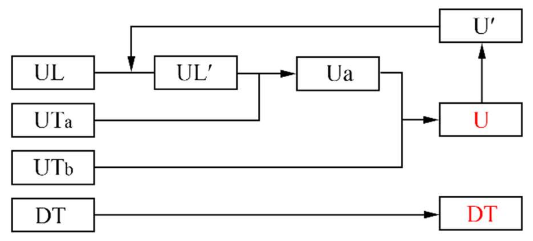
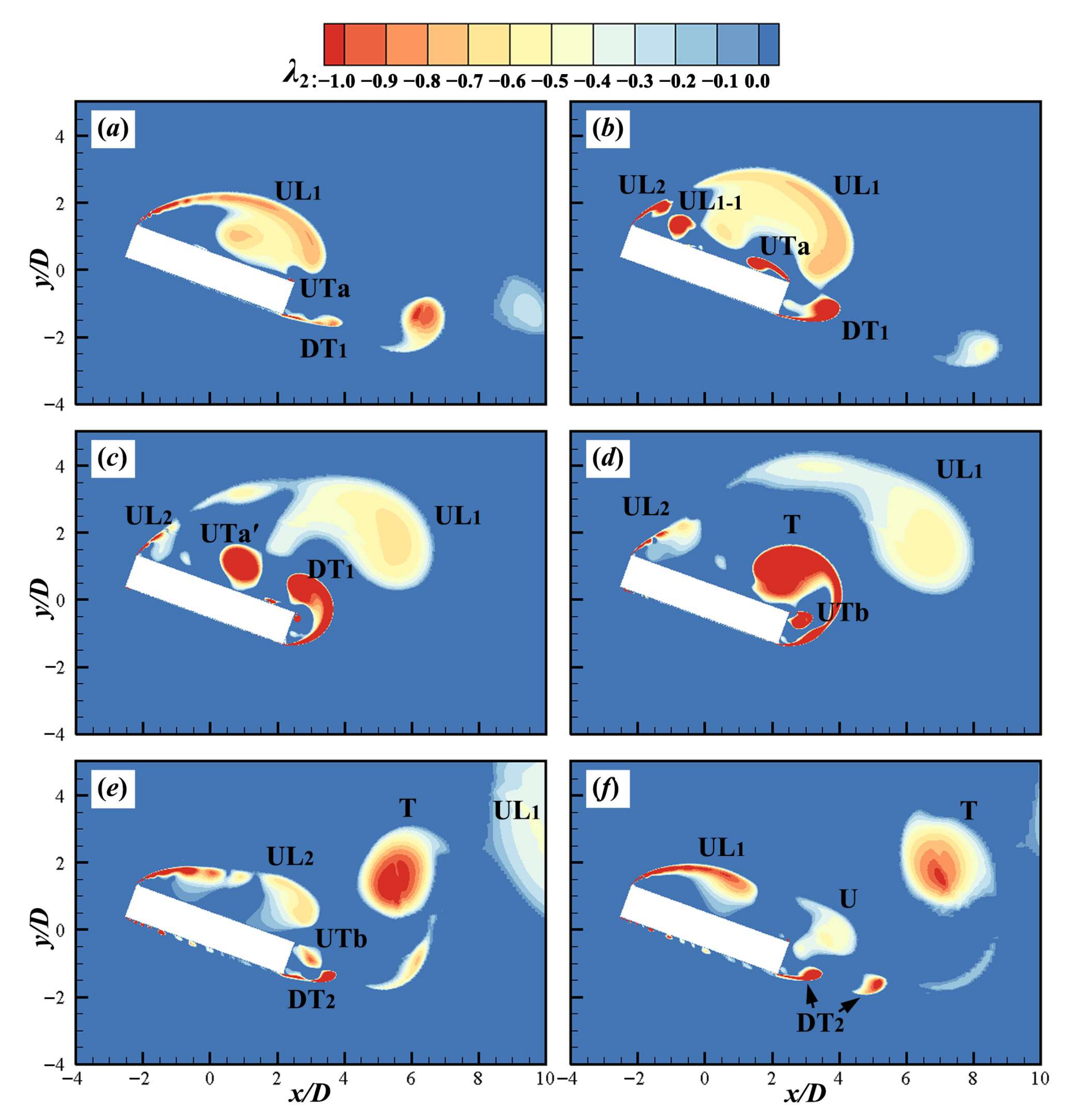
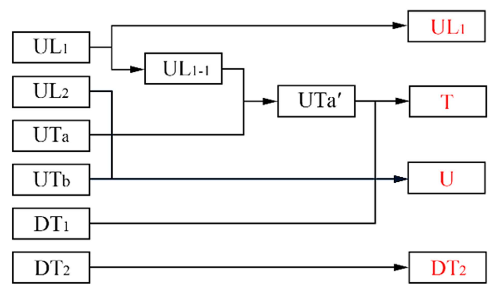
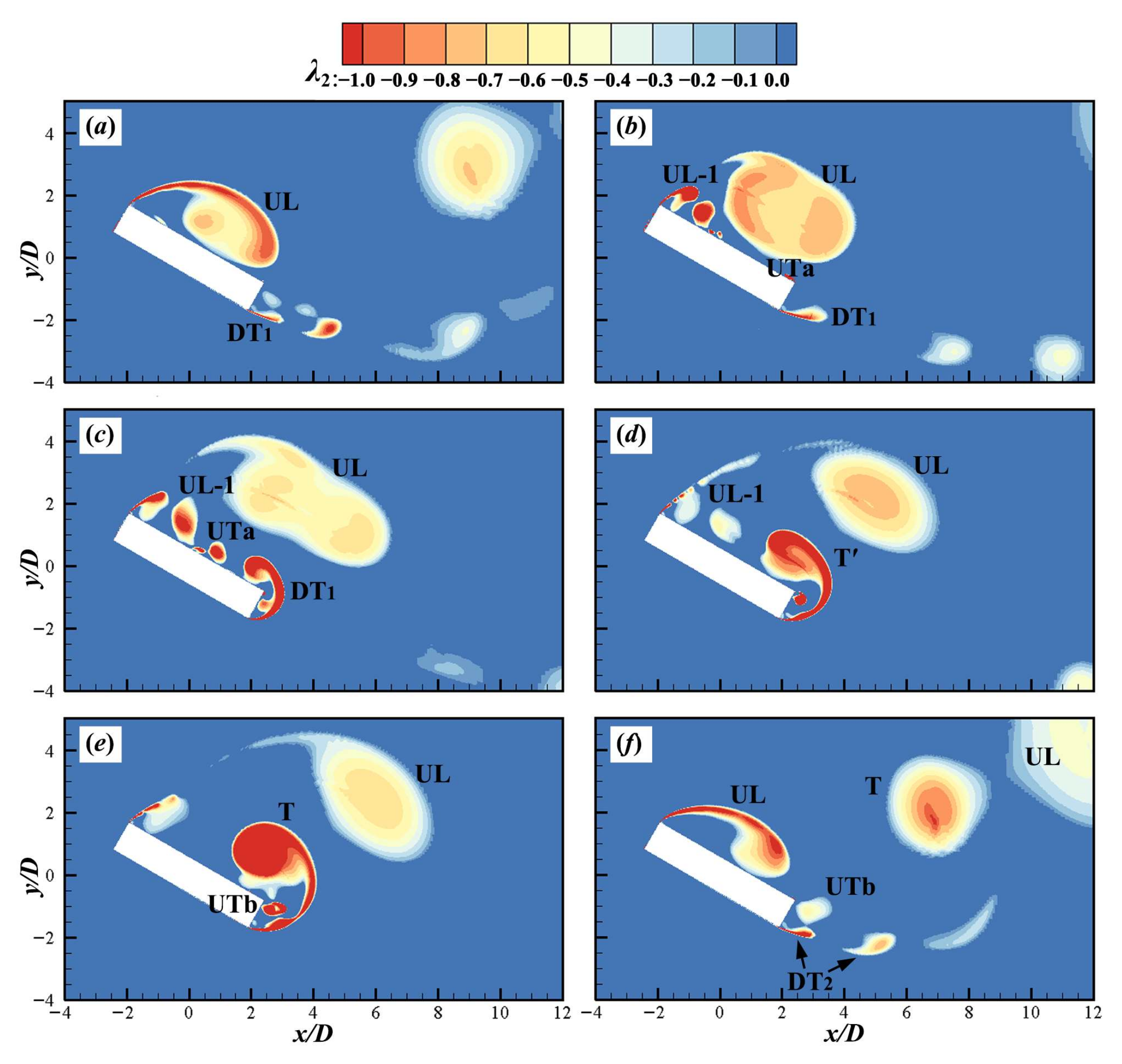
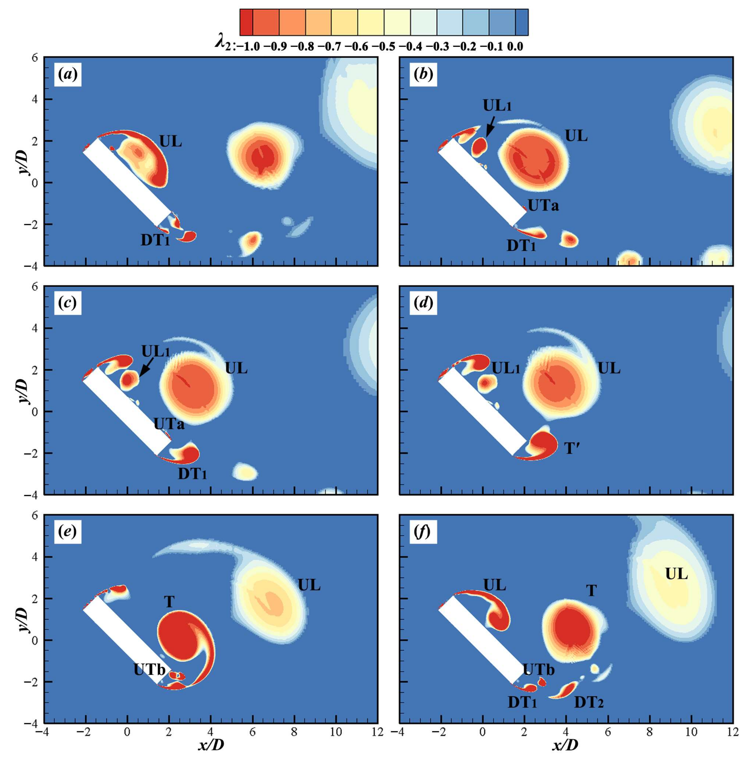
3.4. Vortex Shedding Modes

As the vortices are critical while analyzing the time-dependent flow characteristics, five modes of flow among different AoAs are classified. Figure 17 shows the main vortex structure when α = 0°. The vortices generated above and below the leading edge of the cylinder are denoted as UL (Up-Leading) and DL (Down-Leading), respectively. Similarly, the vortices generated at the trailing edge are UT (Up-Trailing) and DT (Down-Trailing). Occasionally, the vortices generated at the trailing edge may contain two vortices at the same corner, which are named as UTa and UTb, respectively. The instantaneous vortex shedding of the cylinder within a period is shown in Figure 18. Due to the interaction of the main recirculation bubble and the wake recirculation bubble, the upper trailing-edge corner of the cylinder generates two vortices (UTa and UTb), which continue to develop and eventually merge to form a new UT vortex (Figure 18a,b). Then, the UT vortex merges with the UL vortex developed from the leading edge and forms the U vortex (Figure 18c,d). At α = 0°, vortex shedding near the top and bottom sides of the cylinder experiences an identical process of development, finally forming a Kármán vortex street (U vortex + D vortex) in the wake. In this study, this classical vortex shedding mode is named “U-D mode,” and its schematic diagram is shown in Figure 19.

Figure 20 shows the instantaneous vortex shedding process around the cylinder within a period as the AoA increases to 5°. Unlike the results at α = 0°, the UL vortex initially merges with the U′ vortex, which is generated during the previous vortex shedding period to form the UL′ vortex (Figure 20a,b). Then the UL′ vortex merges with the UTa vortex generated by the upper trailing edge to form the U vortex (Figure 20b,c). The DL vortex generated at the lower leading edge sheds to the lower trailing edge and merges with the DT vortex to form the D vortex (Figure 20d,e), and immediately merges with the UTb vortex that slips from the upper trailing-edge corner to the lower trailing-edge corner to generate the T vortex (Figure 20e,f), which sheds and develops downstream.

The instantaneous vortex shedding process around the cylinder with α = 10° is shown in Figure 21. It can be observed that the vortex shedding pattern is similar to that of the cylinder at α = 5°. There is a slight flap in the development of the upper leading-edge UL vortex, which increases its dissipation, and this enlarges the vortex area and decreases vortex intensity. Due to the increase in the AoA, the bottom side of the cylinder gradually changes to the upstream surface, which makes the down leading-edge DL vortex area decrease.

At α = 5° and 10°, the vortices generated on the top side of the cylinder (UL and UTa vortex) merge with each other and shed off, while the vortices generated on the leeward side (UTb vortex) and the bottom side (DL and DT vortex) merge with each other and shed off, forming a Kármán vortex street in the wake. In this study, this vortex shedding mode is named “U-T mode,” and the schematic diagram for this vortex shedding is shown in Figure 22.

Figure 23 shows the instantaneous vortex shedding of the cylinder within a period at α = 15°. The UL vortex generated at the upper leading-edge corner merges with the U′ remaining on the top side during the previous vortex shedding period to form the UL′ vortex (Figure 23a–c). The UL′ vortex merges with the UTa vortex, which is generated at the upper trailing edge, to form the Ua vortex (Figure 23c,d). After the Ua vortex sheds off, it merges with the UTb vortex generated at the upper trailing edge to form the U vortex (Figure 23d,e). A new U′ vortex prepares to be separated from the U vortex, and a UTa vortex is generated at the upper trailing edge (Figure 23f). When it comes to the flow near the lower leading edge, only minute vortices with low intensity are generated and can be ignored. The DT vortex generated at the lower trailing edge sheds directly into the wake without participating in the merge process with other vortices (Figure 23e,f).

When α = 15°, the vortices generated on the top side of the cylinder merge and then shed off, and the vortices generated on the bottom side shed off directly, forming a Kármán vortex street in the wake. In this study, this vortex shedding mode is named “U-DT mode,” and the schematic diagram of this vortex shedding is shown in Figure 24.

The instantaneous vortex shedding around the cylinder at α = 20° in a period is plotted in Figure 25. Development of the UL₁ vortex arising from the upper leading edge of the cylinder provoked the generation of UL_1-1, which then merges with the UTa vortex forming the UTa′ vortex that is attached to the top side (Figure 25a–c). Finally, the UTa′ merges with the DT₁ vortex generated near the lower trailing-edge corner to form a T vortex, which then sheds off (Figure 25c,d). The UL₂ vortex generated at the upper leading-edge corner developed and merged with the UTb vortex generated at the upper trailing edge to form the U vortex (Figure 25e,f). The DT₂ vortex is generated near the lower trailing edge and sheds off directly into the wake (Figure 25f).

When α = 20°, the vortices generated on the upper leading-edge corner (UL₁ vortex) and lower trailing-edge corner (DT₂ vortex) shed off directly. The vortices generated again on those positions (UL₂ vortex and DT₁ vortex) merge with the vortices generated on the upper trailing-edge corner (UTa vortex and UTb vortex), finally forming a Kármán vortex street with four vortices as a period. In this study, this vortex shedding mode is named “UL-T-U-DT mode,” and the schematic diagram of vortex shedding is shown in Figure 26.

Figure 27 shows the instantaneous vortex shedding of the cylinder in a period when α = 30°. During the development process, the UL vortex generated at the upper leading edge directly sheds and spontaneously forms another smaller UL₁ vortex under its influence (Figure 27a,b). The DT₁ vortex generated at the lower trailing edge merges with the UTa vortex generated at the upper leading edge to form a T′ vortex attached to the top side (Figure 27c,d). The T′ vortex merges with a smaller UL₁ vortex to form the T vortex and then sheds (Figure 27d,e). The UTb vortex generated at the upper trailing edge and the DT₂ vortex generated at the lower trailing edge shed off directly into the wake (Figure 27f).

Figure 28 shows the instantaneous vortex shedding of the cylinder when α = 45°. This vortex-shedding mode is the same as that at α = 30°. During the development of the upper leading-edge UL vortex, the flapping amplitude of the vortex increases, and the vortex intensity decreases. No vortex is formed near the lower leading-edge corner, whereas multiple vortices are generated near the lower trailing-edge corner and shed off directly.

At α = 30° and 45°, the vortex shedding mode is very similar to that at α = 20°. These two cases also form the Kármán vortex street with four vortices as a period, and there are directly shedding vortices at the upper leading-edge corner (UL vortex) and lower trailing-edge corner (DT₂ vortex), respectively. However, the other two vortices (T vortex and UTb vortex) are generated in different ways. In this study, this vortex shedding mode is named “UL-T-UTb-DT mode,” and the schematic diagram of the vortex shedding is shown in Figure 29.

A summary of the two primary modes and five sub-modes of vortex shedding at different AoAs is listed in

Table 4. Summary of vortex shedding modes.

α	Mode	UT Characteristic	UL Characteristic	Vortex Street Characteristic
0°	U-D	UTa & UTb	The UL-vortex flaps slightly.	“1 + 1” Kármán vortex street
5°	U-T	UTa & UL
10°		UTb & DT
15°	U-DT	UT & UL
20°	UL-T-U-DT	UTa & DT	The UL-vortex flaps and generates a secondary vortex.	“2 + 2” Kármán vortex street
30°	UL-T- UTb-DT	UTb & UL
45°		UTa & DT

. The analysis shows that when α = 0°~15°, the vortices generated at the upper trailing-edge corner of the cylinder are merged with the adjacent vortices. With the increase in the AoA, the vortex flapping amplitude at the upper leading-edge corner also increases, finally forming a “1 + 1” Kármán vortex street. In the AoA range of 15°~45°, the vortex generated at the upper trailing edge interval merges with the other vortices. During the development of the upper leading-edge vortex, the vortex flap amplitude gradually increases with the increase of the AoA and splits to form new secondary vortices, finally forming a “2 + 2” Kármán vortex street. As an intermediate condition, the flow at α = 15° contains features from the results at α = 10° and α = 20°. When α = 15°, the vortex on the upper leading edge merges with the UTa vortex initially and then merges with the UTb vortex. Although the vortex merges with the adjacent vortex (an example can be found at α = 10°), the merge between the vortex on the upper leading edge and the UTb vortex appears for the first time, which is the main feature of the UL-T-U-DT mode (α = 20°).

4. Conclusions

The separated and reattaching flow around a 5:1 rectangular cylinder at different angles of attack (AoAs) is investigated. The effects of the AoA on the force coefficient, pressure, and flow structure are analyzed. The two primary modes with five sub-modes are identified. The main findings can be summarized as follows:

(1) Both ${\overline{C}}_l$ and ${\overline{C}}_d$ present an overall increasing trend except for the ${\overline{C}}_l$ at AoAs from 10° to 15°, which decrease slightly. Two stages of linear increase in ${\overline{C}}_d$ were observed that are separated by α = 15°, i.e., the slope for α > 15° is steeper than that at α < 15°. Furthermore, the leading-edge vortex shed from the top side corner of the cylinder, and the trailing-edge vortex shed from the bottom side corner have primary influence on the lift and drag forces, respectively.

(2) With the increase in the AoA, the x′-length of the main recirculation bubble on the top side and the distance between the center of the bubble and the leading edge of the cylinder show a trend of increasing initially and then decreasing, and both reach their maximum at α = 15°. Similar characteristics of variation are also observed for the standard deviations ${\sigma }_{x\prime }$ and ${\sigma }_{y\prime }$. Additionally, when α ≥ 15°, the maximum value of ${\sigma }_{x\prime }$ basically remains the same, while that of ${\sigma }_{y\prime }$ gradually increases.

(3) With the increase in the AoA, the maximum positive pressure gradually increases, while the minimum negative pressure gradually decreases, except for α = 15°, which is significantly consistent with the trend of variation in lift and drag forces. The area of high pressure remains almost invariant at α = 0°~15°, beyond which a continuous increase is observed. The area of negative pressure keeps increasing as the AoA increases from 0° to 15°.

(4) The two primary modes are classified based on the number of vortices shed from the cylinder, namely “1 + 1” mode (α = 0°~15°) and “2 + 2” mode (α = 15°~45°). According to the interactions between the vortices, five sub-modes are identified, which include U-D mode (α = 0°), U-T mode (α = 5°~10°), U-DT mode (α = 15° transition mode), UL-T-U-DT mode (α = 20°), and UL-T- UTb-DT mode (α = 30°~45°).

References

1. Bruno, L.; Fransos, D.; Coste, N.; Bosco, A. 3D flow around a rectangular cylinder: A computational study. J. Wind Eng. Ind. Aerod. 2010, 98, 263–276. [Google Scholar] [CrossRef] [Green Version]
2. Bruno, L.; Coste, N.; Fransos, D. Simulated flow around a rectangular 5:1 cylinder: Spanwise discretisation effects and emerging flow features. J. Wind Eng. Ind. Aerod. 2012, 104, 203–215. [Google Scholar] [CrossRef]
3. Schewe, G. Reynolds-number-effects in flow around a rectangular cylinder with aspect ratio 1:5. J. Fluid Struct. 2013, 39, 15–26. [Google Scholar] [CrossRef]
4. Patruno, L.; Ricci, M.; De Miranda, S.; Ubertini, F. Numerical simulation of a 5:1 rectangular cylinder at non-null angles of attack. J. Wind Eng. Ind. Aerod. 2016, 151, 146–157. [Google Scholar] [CrossRef]
5. Mannini, C.; Marra, A.M.; Pigolotti, L.; Bartoli, G. The effects of free-stream turbulence and angle of attack on the aerodynamics of a cylinder with rectangular 5:1 cross section. J. Wind Eng. Ind. Aerod. 2017, 161, 42–58. [Google Scholar] [CrossRef]
6. Ricci, M.; Patruno, L.; de Miranda, S.; Ubertini, F. Flow field around a 5:1 rectangular cylinder using LES: Influence of inflow turbulence conditions, spanwise domain size and their interaction. Comput. Fluids 2017, 149, 181–193. [Google Scholar] [CrossRef]
7. Wu, B.; Li, S.; Cao, S.; Yang, Q.; Zhang, L. Numerical investigation of the separated and reattaching flow over a 5:1 rectangular cylinder in streamwise sinusoidal flow. J. Wind Eng. Ind. Aerodyn. 2020, 198, 104120. [Google Scholar] [CrossRef]
8. Wu, B.; Li, S.; Li, K.; Zhang, L. Numerical and experimental studies on the aerodynamics of a 5:1 rectangular cylinder at angles of attack. J. Wind Eng. Ind. Aerodyn. 2020, 199, 104097. [Google Scholar] [CrossRef]
9. Lou, X.; Sun, C.; Jiang, H.; Zhu, H.; An, H.; Zhou, T. Three-Dimensional Direct Numerical Simulations of a Yawed Square Cylinder in Steady Flow. J. Mar. Sci. Eng. 2022, 10, 1128. [Google Scholar] [CrossRef]
10. Li, D.; Yang, Q.; Ma, X.; Dai, G. Free Surface Characteristics of Flow around Two Side-by-Side Circular Cylinders. J. Mar. Sci. Eng. 2018, 6, 75. [Google Scholar] [CrossRef]
11. Han, X.; Wang, J.; Zhou, B.; Zhang, G.; Tan, S.-K. Numerical Simulation of Flow Control around a Circular Cylinder by Installing a Wedge-Shaped Device Upstream. J. Mar. Sci. Eng. 2019, 7, 422. [Google Scholar] [CrossRef] [Green Version]
12. Wang, W.; Mao, Z.; Tian, W.; Zhang, T. Numerical Investigation on Vortex-Induced Vibration Suppression of a Circular Cylinder with Axial-Slats. J. Mar. Sci. Eng. 2019, 7, 454. [Google Scholar] [CrossRef] [Green Version]
13. Piran, F.; Karampour, H.; Woodfield, P. Numerical Simulation of Cross-Flow Vortex-Induced Vibration of Hexagonal Cylinders with Face and Corner Orientations at Low Reynolds Number. J. Mar. Sci. Eng. 2020, 8, 387. [Google Scholar] [CrossRef]
14. Anwar, M.U.; Lashin, M.M.A.; Khan, N.B.; Munir, A.; Jameel, M.; Muhammad, R.; Guedri, K.; Galal, A.M. Effect of Variation in the Mass Ratio on Vortex-Induced Vibration of a Circular Cylinder in Crossflow Direction at Reynold Number = 104: A Numerical Study Using RANS Model. J. Mar. Sci. Eng. 2022, 10, 1126. [Google Scholar] [CrossRef]
15. Nazvanova, A.; Yin, G.; Ong, M.C. Numerical Investigation of Flow around Two Tandem Cylinders in the Upper Transition Reynolds Number Regime Using Modal Analysis. J. Mar. Sci. Eng. 2022, 10, 1501. [Google Scholar] [CrossRef]
16. Taheri, E.; Zhao, M.; Wu, H. Numerical Investigation of the Vibration of a Circular Cylinder in Oscillatory Flow in Oblique Directions. J. Mar. Sci. Eng. 2022, 10, 767. [Google Scholar] [CrossRef]
17. Wang, T.; Yang, Q.; Tang, Y.; Shi, H.; Zhang, Q.; Wang, M.; Epikhin, A.; Britov, A. Spectral Analysis of Flow around Single and Two Crossing Circular Cylinders Arranged at 60 and 90 Degrees. J. Mar. Sci. Eng. 2022, 10, 811. [Google Scholar] [CrossRef]
18. Bartoli, G.; Bruno, L.; Buresti, G.; Ricciardelli, F.; Salvetti, M.V.; Zasso, A. BARC Overview Document. 2008. Available online: http://www.aniv-iawe.org/barc (accessed on 17 July 2020).
19. Bruno, L.; Salvetti, M.V.; Ricciardelli, F. Benchmark on the Aerodynamics of a Rectangular 5:1 Cylinder: An overview after the first four years of activity. J. Wind Eng. Ind. Aerodyn. 2014, 126, 87–106. [Google Scholar] [CrossRef] [Green Version]
20. Álvareza, A.J.; Nietoa, F.; Nguyen, D.T.; Owen, J.S.; Hernándeza, S. 3D LES simulations of a static and vertically free-to-oscillate 4:1 rectangular cylinder: Effects of the grid resolution. J. Wind Eng. Ind. Aerodyn. 2019, 192, 31–44. [Google Scholar] [CrossRef]
21. Zhang, Z.; Xu, F. Spanwise length and mesh resolution effects on simulated flow around a 5:1 rectangular cylinder. J. Wind Eng. Ind. Aerodyn. 2020, 202, 104186. [Google Scholar] [CrossRef]
22. Tang, Y.; Hui, Y.; Li, K. LES study on variation of flow pattern around a 4:1 rectangular cylinder and corresponding wind load during VIV. J. Wind Eng. Ind. Aerodyn. 2022, 228, 105121. [Google Scholar] [CrossRef]
23. Mannini, C.; Soda, A.; Voss, R.; Schewe, G. URANS and DES simulation of flow around a rectangular cylinder. New Res. Num. Exp. Fluid Mech. VI 2007, 96, 36–43. [Google Scholar]
24. Mannini, C. Applicability of URANS and DES simulations of flow past rectangular cylinders and bridge sections. Computation 2015, 3, 479–508. [Google Scholar] [CrossRef] [Green Version]
25. Bai, W.; Mingham, C.G.; Causon, D.M.; Qian, L. Detached eddy simulation of turbulent flow around square and circular cylinders on Cartesian cut cells. Ocean Eng. 2016, 117, 1–14. [Google Scholar] [CrossRef]
26. Hong, F.; Xue, H.; Zhang, B. Improved detached-eddy simulation of the turbulent unsteady flow past a square cylinder. AIP Adv. 2020, 10, 125011. [Google Scholar] [CrossRef]
27. Yousif, M.Z.; Lim, H. Improved delayed detached-eddy simulation and proper orthogonal decomposition analysis of turbulent wake behind a wall-mounted square cylinder. AIP Adv. 2021, 11, 045011. [Google Scholar] [CrossRef]
28. Zhang, D. Comparison of Various Turbulence Models for Unsteady Flow around a Finite Circular Cylinder at Re = 20,000. IOP Conf. Ser. J. Phys. Conf. Ser. 2017, 910, 012027. [Google Scholar] [CrossRef]
29. Nietoa, F.; Hargreavesb, D.M.; Owenb, J.S.; Hernándeza, S. On the applicability of 2D URANS and SST k-ω turbulence model to the fluid-structure interaction of rectangular cylinders. Eng. Appl. Comput. Fluid Mech. 2015, 9, 157–173. [Google Scholar]
30. Gorle, J.M.R.; Chatellier, L.; Pons, F.; Ba, M. Flow and performance analysis of H-Darrieus hydroturbine in a confined flow: A computational and experimental study. J. Fluids Struct. 2016, 66, 382–402. [Google Scholar] [CrossRef]
31. Gorle, J.M.R.; Chatellier, L.; Pons, F.; Ba, M. Modulated circulation control around the blades of a vertical axis hydrokinetic turbine for flow control and improved performance. Renew. Sustain. Energy Rev. 2019, 105, 363–377. [Google Scholar] [CrossRef]
32. Mannini, C.; Šoda, A.; Schewe, G. Unsteady RANS modelling of flow past a rectangular cylinder: Investigation of Reynolds number effects. Comput. Fluids 2010, 39, 1609–1624. [Google Scholar] [CrossRef] [Green Version]
33. Matsumoto, M.; Yagi, T.; Tamaki, H.; Tsubota, T. Vortex-induced vibration and its effect on torsional flutter instability in the case of B/D=4 rectangular cylinder. J. Wind Eng. Ind. Aerodyn. 2008, 96, 971–983. [Google Scholar] [CrossRef]
34. Zhang, Q.; Liu, Y. Separated flow over blunt plates with different chord-to-thickness ratios: Unsteady behaviors and wall-pressure fluctuations. Exp. Therm. Fluid Sci. 2017, 84, 199–216. [Google Scholar] [CrossRef]
35. Carassale, L. Flow-induced actions on cylinders in statistically-symmetric cross flow. Probab. Eng. Mech. 2009, 24, 288–299. [Google Scholar] [CrossRef]
36. Menter, F.R. Zonal two equation k-ω turbulence models for aerodynamic flows. In Proceedings of the 23rd Fluid Dynamics, Plasmadynamics, and Lasers Conference, Orlando, FL, USA, 6–9 July 1993; Volume 93, p. 2906. [Google Scholar]
37. Menter, F.R. Two-equation eddy-viscosity turbulence models for engineering applications. AIAA J. 1994, 32, 1598–1605. [Google Scholar] [CrossRef] [Green Version]
38. Menter, F.R.; Kuntz, M.; Langtry, R. Ten years of industrial experience with the SST turbulence model. Turbul. Heat Mass Transf. 2003, 4, 625–632. [Google Scholar]
39. Zhang, D.; Cheng, L.; An, H.; Draper, S. Flow around a surface-mounted finite circular cylinder completely submerged within the bottom boundary layer. Eur. J. Mech. B-Fluid. 2021, 86, 169–197. [Google Scholar] [CrossRef]
40. Bruno, L.; Salvetti, M.V. Benchmark on the Aerodynamics of a Rectangular 5:1 Cylinder (BARC): Description, Test Case Studies, Evaluation, and Best Practice Advice. 2017. Available online: http://www.kbwiki.ercoftac.org/w/index.php/Abstr:UFR_2-15 (accessed on 24 October 2020).
41. Galli, F. Aerodynamic Behaviour of Bluff Line-like Structures: Experimental and Computational Approach. Master’s Thesis, Politecnico di Torino, Turin, Italy, 2005. [Google Scholar]
42. Ribeiro, A.F.P. Unsteady RANS modelling of flow past a rectangular 5:1 cylinder: Investigation of edge sharpness effects. In Proceedings of the 13th International Conference on Wind Engineering, Amsterdam, The Netherlands, 10–15 July 2011. [Google Scholar]
43. Grozescu, A.N.; Bruno, L.; Fransos, D.; Salvetti, M.V. Large-eddy simulations of a Benchmark on the Aerodynamics of a Rectangular 5:1 Cylinder. In Proceedings of the 20th Italian Conference on Theoretical and Applied Mechanics, Bologna, Italy, 12–15 September 2011; Available online: https://arpi.unipi.it/handle/11568/238156 (accessed on 24 October 2020).
44. Grozescu, A.N.; Salvetti, M.V.; Camarri, S.; Buresti, G. Variational multiscale large-eddy simulations of the BARC flow configuration. In Proceedings of the 13th International Conference on Wind Engineering, Amsterdam, The Netherlands, 12–15 September 2011. [Google Scholar]
45. Jeong, J.; Hussain, F. On the identification of a vortex. J. Fluid Mech. 1995, 285, 69–94. [Google Scholar] [CrossRef]
Figure 1. Geometric schematics of the computational domain.
Jmse 10 01913 g001
Figure 2. Grid topology and details: (a) mesh in the proximity of the cylinder; (b) close-up of the core region; (c) around the corner; (d) non-dimensional distance s/D of cylinder circumference (taking α = 45° as an example).
Jmse 10 01913 g002
Figure 3. Distribution of the time-averaged pressure coefficient on the top side of the cylinder [41,42].
Jmse 10 01913 g003
Figure 4. Time-averaged velocity contour map and streamline distribution.
Jmse 10 01913 g004
Figure 5. Time-averaged velocity distribution profile near the wall.
Jmse 10 01913 g005
Figure 6. Profiles of time-averaged Reynolds normal stress < u u > / U 2 (left), < v v > / U 2 (middle), and Reynolds shear stress < u v > / U 2 (right). The first, second, third, and fourth rows correspond to locations of x/D = −1.25, 0, 1.25, and 2.5, respectively.
Jmse 10 01913 g006
Figure 7. Time histories of lift coefficient and drag coefficient under different AoAs. (a) α = 0°, (b) α = 5°, (c) α = 10°, (d) α = 15°, (e) α = 20°, (f) α = 30°, (g) α = 45°.
Jmse 10 01913 g007
Figure 8. Time-average (a) lift coefficient, (b) drag coefficient, and (c) Strouhal number at different AoAs.
Jmse 10 01913 g008
Figure 9. Instantaneous vortex structure with maximum lift coefficient at various AoAs. (a) α = 0°, (b) α = 5°, (c) α = 10°, (d) α = 15°, (e) α = 20°, (f) α = 30°, (g) α = 45°.
Jmse 10 01913 g009
Figure 10. Instantaneous vortex structure with maximum drag coefficient at various AoAs. (a) α = 0°, (b) α = 5°, (c) α = 10°, (d) α = 15°, (e) α = 20°, (f) α = 30°, (g) α = 45°.
Jmse 10 01913 g010
Figure 11. Time-averaged streamwise velocity contour and time-averaged streamline distribution. (a) α = 0°, (b) α = 5°, (c) α = 10°, (d) α = 15°, (e) α = 20°, (f) α = 30°, (g) α = 45°, (h) The trend of LR or LC with the increase in the AoA.
Jmse 10 01913 g011
Figure 12. Time-averaged pressure p ¯ distribution at different AoA (+ represents the location of the maximum and minimum values, and the blue and red lines represent the contours with p ¯ * = −0.4 and p ¯ * = 0.4, respectively). (a) α = 0°, (b) α = 5°, (c) α = 10°, (d) α = 15°, (e) α = 20°, (f) α = 30°, (g) α = 45°, (h) The trend of p ¯ * with the increase in the AoA.
Jmse 10 01913 g012
Figure 13. Schematic diagram of (a) cross-section distribution and (b) velocity decomposition (red is the global coordinate system, and blue is the local coordinate system).
Jmse 10 01913 g013
Figure 14. Time-averaged velocity U ¯ x distribution of each section. (a) x′/D = −2.5, (b) x′/D = −1.0, (c) x′/D = 1.0, (d) x′/D = 2.5.
Jmse 10 01913 g014
Figure 15. The standard deviation of time-averaged velocity: (a) velocity along the direction of the cylinder, (b) velocity in the direction perpendicular to the cylinder.
Jmse 10 01913 g015
Figure 16. Time-average pressure coefficient distribution on the cylinder wall.
Jmse 10 01913 g016
Figure 17. Schematic diagram of vortex naming.
Jmse 10 01913 g017
Figure 18. Vortex evolution within a vortex shedding period at α = 0°. (a) tU/D = 859.9, (b) tU/D = 861.3, (c) tU/D = 862.0, (d) tU/D = 863.4, (e) tU/D = 864.8, (f) tU/D = 866.2.
Jmse 10 01913 g018
Figure 19. The schematic diagram of vortex evolution in U-D mode.
Jmse 10 01913 g019
Figure 20. Vortex evolution within a vortex shedding period at α = 5°. (a) tU/D = 872.4, (b) tU/D = 874.2, (c) tU/D = 875.1, (d) tU/D = 876.0, (e) tU/D = 876.9, (f) tU/D = 878.7.
Jmse 10 01913 g020
Figure 21. Vortex evolution within a vortex shedding period at α = 10°. (a) tU/D = 855.4, (b) tU/D = 856.4, (c) tU/D = 858.4, (d) tU/D = 859.9, (e) tU/D = 861.4, (ff) tU/D = 863.4.
Jmse 10 01913 g021
Figure 22. The schematic diagram of vortex evolution in U-T mode.
Jmse 10 01913 g022
Figure 23. Vortex evolution within a vortex shedding period at α = 15°. (a) tU/D = 881.0, (b) tU/D = 884.0, (c) tU/D = 886.0, (d) tU/D = 891.0, (e) tU/D = 896.0, (f) tU/D = 899.0.
Jmse 10 01913 g023
Figure 24. The schematic diagram of vortex evolution in U-DT mode.
Jmse 10 01913 g024
Figure 25. Vortex evolution within a vortex shedding period at α = 20°. (a) tU/D = 849.0, (b) tU/D = 855.0, (c) tU/D = 859.0, (d) tU/D = 861.0, (e) tU/D = 867.0, (f) tU/D = 871.0.
Jmse 10 01913 g025
Figure 26. The schematic diagram of vortex evolution in UL-T-U-DT mode.
Jmse 10 01913 g026
Figure 27. Vortex evolution within a vortex shedding period at α = 30°. (a) tU/D = 822.2, (b) tU/D = 828.6, (c) tU/D = 833.4, (d) tU/D = 836.4, (e) tU/D = 838.0, (f) tU/D = 844.0.
Jmse 10 01913 g027
Figure 28. Vortex evolution within a vortex shedding period at α = 45°. (a) tU/D = 825.7, (b) tU/D = 832.9, (c) tU/D = 835.3, (d) tU/D = 836.5, (e) tU/D = 840.1, (f) tU/D = 843.7.
Jmse 10 01913 g028
Figure 29. The schematic diagram of vortex evolution in UL-T- UTb-DT mode.
Jmse 10 01913 g029