Calibration and Validation of Two Tidal Sand Wave Models: A Case Study of The Netherlands Continental Shelf

Abstract

Tidal sand waves form a dynamic bed pattern, widely occurring in shallow shelf seas such as the North Sea. Their importance to coastal engineering has inspired many advances in process-based sand wave modelling, aimed at explaining physical mechanisms in the formation stage (‘linear regime’) and capturing the finite amplitude evolution to equilibrium states (‘nonlinear regime’). However, systematic validation of particularly the nonlinear sand wave models is still lacking. Here, we perform a two-step calibration and validation study of a sand wave model (specifically, their linear and nonlinear model versions) against field data from the North Sea. In the first step, the linear model is calibrated by seeking overall values of two uncertain input parameters (slip parameter, wave period) for which the modeled and observed wavelengths show the best agreement. In the second step, using the calibrated input parameters and preferred wavelengths from the linear model, equilibrium heights from the nonlinear sand wave model are validated against the observed sand wave heights. Our results show satisfactory agreement between observed and modeled sand wave lengths (from the linear sand wave model) and a systematic overprediction of sand wave heights (using the nonlinear model). Regression analysis can be used to rescale the nonlinear model results to obtain realistic predictions of sand wave heights.

1. Introduction

Shallow shelf seas are dynamic systems and are intensively used. For example, the North Sea is used for navigation, fisheries, hydrocarbon extraction, wind farming, recreation, military exercising, and sand extraction (see, e.g., [1,2,3,4,5]), which require careful planning and maintenance. Some of these activities, such as dredging, beam-trawl fishing, and the construction of offshore wind farms, pipelines, and communication cables, interfere with the seabed (see, e.g., [6,7,8]). At the same time, the seabed is dynamic in itself due to the complex interplay of tides, waves, and the sediment of the seabed. This implies autonomous behavior as well as a response to intervention [9], both of which must be taken into account when assessing the impact of such engineering activities.

A typical example of seabed dynamics is expressed in the occurrence of tidal sand waves. These are large-scale bedforms, occurring as more or less rhythmic patterns with typical wavelengths of hundreds of meters, heights of several meters, and usually asymmetric shapes (e.g., [10,11,12]). Tidal sand waves evolve over time scales of the order of years and, depending on the flow conditions, may migrate at rates up to tens of meters per year. It is this combination of their widespread occurrence, dimensions and dynamics that make tidal sand waves highly relevant for engineering purposes. Overall, there is a need to understand sand wave dynamics, both autonomously and in response to human intervention.

Tidal sand waves have been explained as instabilities of a flat sandy seabed subject to tidal motion [13,14]. For more information on how linear and nonlinear stability approaches help in understanding rhythmic features in general and in particular sand waves, we refer the reader to Dodd et al. [15]. The instability is driven by vertical recirculating cells that result from tide–topography interactions, enhancing sediment transport from trough to crest. This mechanism was studied using linear stability analysis of an idealized morphodynamic model with a strongly schematized description of tidal flow and sediment transport [14] and later extended to account for the effects of residual currents [16], tidal asymmetry [17], suspended sediment transport [18], wave and wind forcing [19], and bio-morphological interaction [20]. The typical output of a linear model is preferred wavelength, orientation, and migration rate in the initial stages of development. Furthermore, these linear sand wave models have been validated regarding their occurrence [21], wavelengths [22,23], migration rates [24,25], sediment grain sizes [2], and the influence of wave climate on sand wave properties [26]. However, the validity of such linear models is restricted to the small amplitude regime, making them unable to capture practically relevant properties of sand waves in equilibrium, such as their shapes and heights. Notably, those properties are the most relevant for many practical engineering applications.

To capture the evolution towards a finite amplitude equilibrium, various nonlinear model studies have been developed (e.g., [27,28,29,30,31]). Model results show convergence to equilibrium shapes with realistic shapes, but heights are usually overestimated. Suspended sediment transport is found to stabilize and reduce sand wave heights [32]. Moreover, Terwindt [10] found from observations that frequently during stormy winters, sand wave heights decreased, likely due to high waves. Campmans et al. [30] showed that including wind wave effects indeed suppresses the modeled equilibrium heights of tidal sand waves. In all of these nonlinear models, computational time is a challenge, which forces schematization of the model domain type (2DV) and size (e.g., spatially periodic boundary conditions on a relatively short domain), solution method (morphological acceleration factors), and/or the extent of sensitivity analyses.

Despite the increasing number of nonlinear model studies on tidal sand waves, systematic quantitative validation of these nonlinear models against field data is still sparse. Krabbendam et al. [31] calibrated a nonlinear sand wave model for one transect of sand waves in the North Sea, and validated this for three other transects. Such applications are sparse because of the idealized nature of the current sand wave models, which makes them very suitable for systematic analysis of physical mechanisms, but less so for application to a field site with local geometry and specific in situ conditions. This is further complicated by the model schematizations imposed by the aforementioned computational limitations. Finally, the temporal resolution of topographic surveys is limited and long-term forcing conditions (not only tides, wind and waves as well) are surrounded by large uncertainties.

The objective of this paper is to quantitatively calibrate and validate two existing sand wave models [19,30] with field data from the Netherlands Continental Shelf [12,33] containing spatially varying data on local environmental conditions and the observed sand wave characteristics. In particular, we aim to answer the following research questions:

• To what extent can the observed sand wave lengths be reproduced by the linear model?
• To what extent can the observed sand wave heights be reproduced by the nonlinear model?

To answer these questions, we follow a two-step model approach, using the linear model to obtain sand wave lengths (addressing the first research question) and, given these lengths, subsequently using the nonlinear model to obtain sand wave heights (second research question). This is conducted on two disjunct sets of locations, one for calibration and one for validation. From the input parameters, partly based on the local environmental conditions, we use two uncertain input parameters for calibration: slip parameter and wind wave period.

2. Methods

The two-step methodology is schematized in Figure 1, which is further explained in the following subsections.

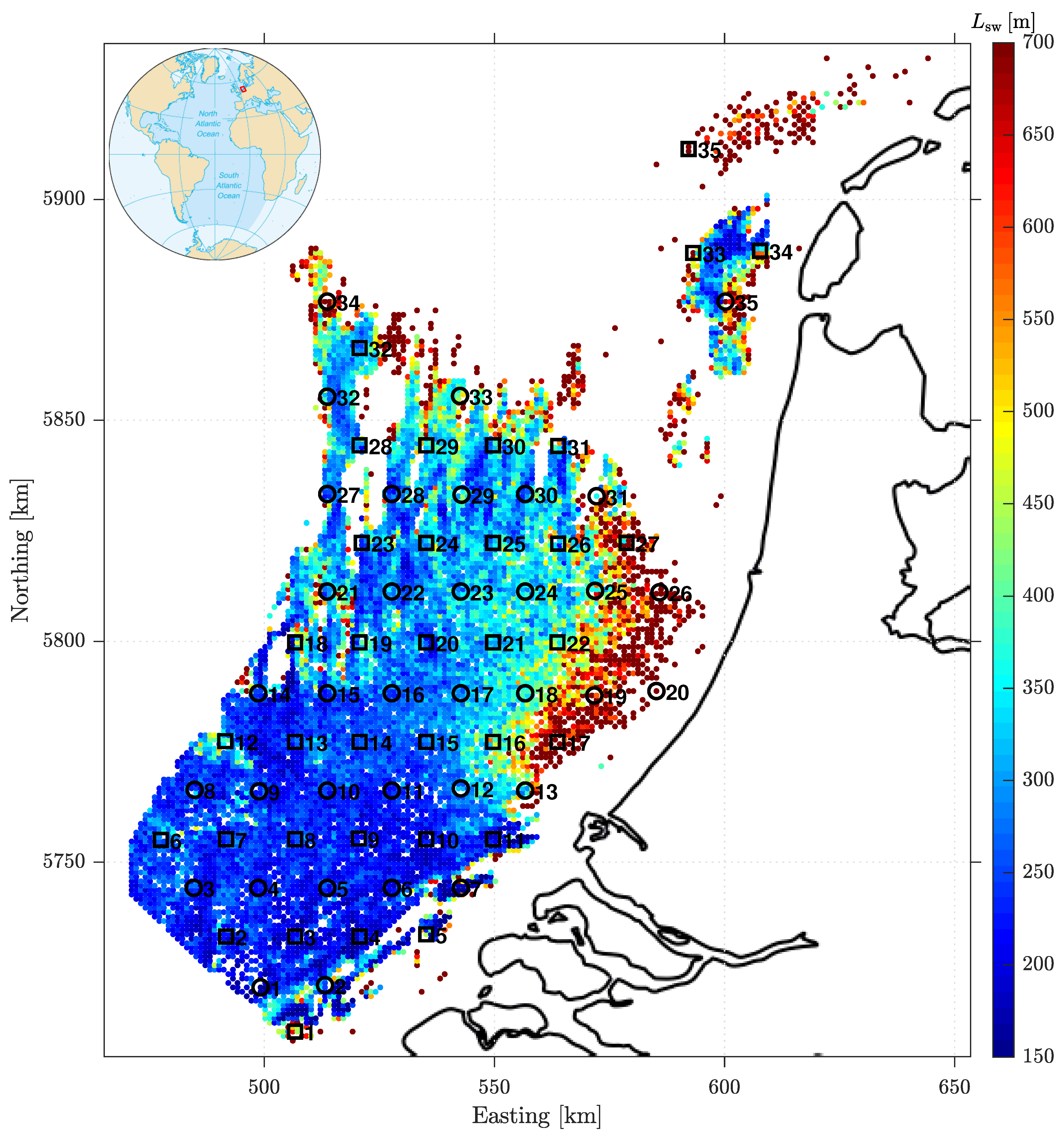
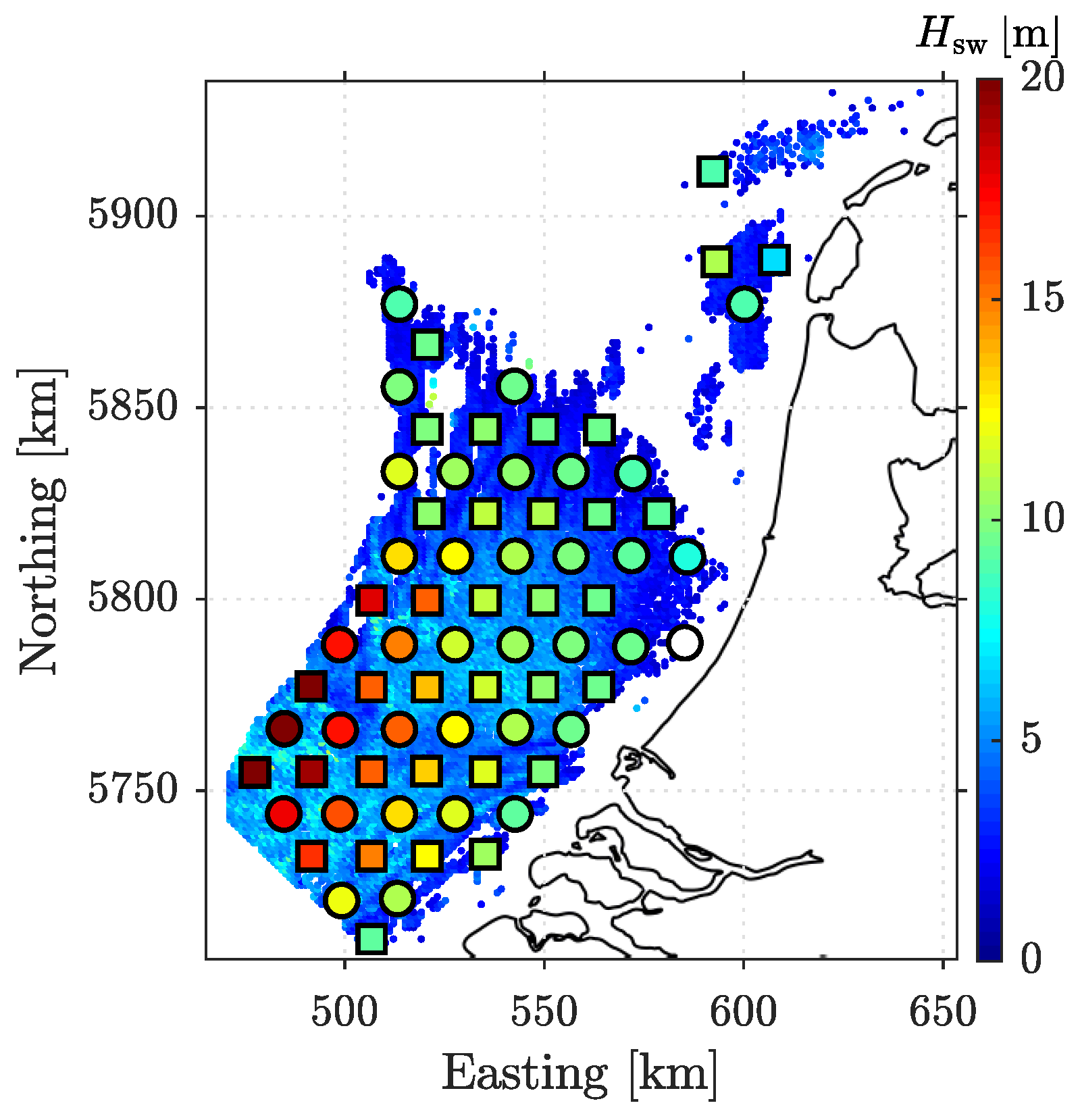
2.1. Sand Wave Data from the Netherlands Continental Shelf

Damen et al. [12,33] quantified the lengths, heights, and asymmetries of all sand waves in the Dutch part of the North Sea by systematically analyzing 25 × 25 m resolution bathymetric data, resulting in 1.5 million data points. Damen et al. [12] created maps of average sand wave characteristics on a resolution of 1 × 1 km. On the same 1 × 1 km resolution, the data set provides local values of water depth, sediment grain size, M2 tidal velocity amplitude, peak velocity asymmetry, and significant wave height. The water depth was determined from bathymetric data, sediment grain size from interpolation of sediment samples [34], and all hydrodynamic parameters from the so-called ZUidelijke NOordzee model (ZUNO) [35], which is driven by the Dutch Continental Shelf Model [36]. The entire data set is publicly available [33].

Next, they determined the correlations between the obtained characteristics with local environmental parameters, such as water depth, sediment grain size, M2 tidal velocity component, the tidal peak velocity difference, and the significant surface wave height. The strongest correlation was found between sand wave characteristics and the Rouse number, pointing to the importance of suspended load sediment transport.

2.2. A Two-Step Model Approach

In this study, both a linear [19] and a nonlinear sand wave model [30] are used. In these two models, tidal currents are described by the shallow water equations, sediment transport is described by a transport formula, and the bed evolution by the Exner equation. Despite the suggested importance of suspended load [12], the nonlinear sand wave model forces us to restrict ourselves to a bed-load type of formulation; see the discussion in Section 4. Detailed model descriptions are given in Campmans et al. [19,30]. Both models are based on the same model equations, but they differ in the solution approach. The linear stability model is a fast way to investigate sand wave characteristics in the formation stage (i.e., small amplitude characteristics). This enables us to perform a large number of model simulations. The nonlinear model requires much more computational time, but it allows to investigate finite amplitude sand wave characteristics, such as sand wave heights and shapes during their evolution to an equilibrium state. Here, we use the two models in a two-step approach, where the linear stability model is used to calculate the sand wave lengths, and the nonlinear model is used to calculate sand wave heights and shapes on a horizontally periodic domain with the domain lengths equal to the sand wave lengths obtained in the first step.

The linear stability model investigates the stability of a flat seabed by analyzing the seabed response to small amplitude wavy perturbations (or modes). If all wavy perturbations decay, the seabed is stable, if at least one perturbation grows, it is unstable. The fastest growing mode is considered to dominate the bed-form length. The possibility of performing a large number of simulations for various North Sea locations, systematically varying some of the (uncertain) input parameters, makes the linear model an ideal tool for a calibration procedure regarding sand wave lengths.

The nonlinear model numerically integrates the model equations in time, allowing the nonlinear finite-amplitude feedback of the seabed onto the hydrodynamics, sediment transport, and finally, seabed evolution. The seabed topography evolves towards its equilibrium shape, from which the sand wave heights and shapes are determined.

2.3. Selection of Calibration and Validation Locations

In order to compare model results to field observations, two grids of points were drawn over the study area, staggered to one another (Figure 2). Only the points in the grids where sand wave characteristics in the data by Damen et al. [12] are available are considered. One of the grids provides calibration locations for sand wave lengths using the linear model. Similarly, the second grid is used for validation. Both the calibration and validation sets consist of 35 locations. The choice of the number of locations is further commented upon in the Discussion (Section 4).

2.4. Model Input

Since both sand wave models require to a large extent the same model input parameters, the model parameters are described generally for both models. Where model parameters differ between the two models, this is stated explicitly. The model parameters are shown in Table 1.

The hydrodynamic model requires a depth-averaged velocity amplitude of the M2 tide $U_{\mathrm{M}2}$ as well as the residual current $U_{\mathrm{M}0}$. Damen et al. [12,33] provide the M2 tidal velocity amplitude, as well as the tidal peak velocity asymmetry, which is the averaged difference between the magnitudes of the ebb and flood current. Here, we fully attribute this asymmetry to an M0 tidal current $U_{\mathrm{M}0}$ of half this difference, thereby ignoring possible effects of overtides.

The models solve a depth-dependent flow profile which depends on a turbulence model with a constant eddy viscosity $A_{\mathrm{v}}$, a slip parameter S, with a partial slip condition at the seabed:

$$A_{\mathrm{v}}\frac{\partial u}{\partial z}=Su.$$

(1)

The eddy viscosity $A_{\mathrm{v}}$ is estimated using the water depth H and tidal velocity amplitude $U_{\mathrm{M}2}$ (e.g., [37,38])

$$A_{\mathrm{v}}=c{U}_{\mathrm{M}2}H,$$

(2)

where $c=2.5\times {10}^{-3}$. For each model location, the water depth H and the M2 tidal velocity amplitude $U_{\mathrm{M}2}$ are taken from Damen et al. [12,33].

Figure 2. The calibration (circles) and validation (squares) locations determined using two staggered grids. The colored dots indicate observed sand wave lengths at locations where sand waves occur [12,33]. The location of the North Sea is indicated by the red box on the shown globe (By CIA— CIA World Factbook—Atlantic Ocean (picture URL), Public Domain, accessed on 11 November 2022., https://commons.wikimedia.org/w/index.php?curid=7627352).

Figure 2. The calibration (circles) and validation (squares) locations determined using two staggered grids. The colored dots indicate observed sand wave lengths at locations where sand waves occur [12,33]. The location of the North Sea is indicated by the red box on the shown globe (By CIA— CIA World Factbook—Atlantic Ocean (picture URL), Public Domain, accessed on 11 November 2022., https://commons.wikimedia.org/w/index.php?curid=7627352).

For the surface wave height, the significant wave height from the data set [12,33] is used. The wave period is an uncertain parameter, as wind waves typically tend to have a range of wave periods. Additionally, the wave period that is relevant for the free water motion does not have to be the same wave period relevant for the water motion near the bed at tens of meters of water depth. In this model study, the wave period $T_{\mathrm{w}}$ is used as one of the calibration parameters. The partial slip parameter S is an uncertain parameter, which will be used as the second of the two calibration parameters.

Table 1. Overview of input parameters for the linear and nonlinear models.

Model Parameter	Const.	Cal. ${}^{†}$	Local ${}^{*}$	Symbol	Value	Unit
Water depth	·	·	√	H	·	m
Tidal current velocity (M2)	·	·	√	$U_{\mathrm{M}2}$	·	m s${}^{-1}$
Residual current velocity (M0)	·	·	√	$U_{\mathrm{M}0}$	·	m s${}^{-1}$
Tidal frequency (M2)	√	·	·	$\sigma$	$1.41\times {10}^{-4}$	rad s${}^{-1}$
Tidal angle (M0, M2)	√	·	·	${\theta }_{\mathrm{tide}}$	0	${}^{\circ }$
Wave friction factor	√	·	·	$f_{\mathrm{w}}$	0.1	-
Gravitational acceleration	√	·	·	g	9.81	m s${}^{-2}$
Vertical eddy viscosity	·	·	√	$A_{\mathrm{v}}$	$2.5\times {10}^{-3}{U}_{\mathrm{M}2}H$	m${}^2$ s${}^{-1}$
Slip parameter	·	√	·	S	$0.0154{}^{†}$	m s${}^{-1}$
Slope correction factor	√	·	·	$\lambda$	1.5	-
Coriolis parameter	√	·	·	f	0	rad s${}^{-1}$
Tidal ellipticity (M2)	√	·	·	${ϵ}_{\mathrm{M}2}$	0	-
Sediment grain size	·	·	√	d	·	$\mathsf{\mu }$m
Bed load exponent	√	·	·	$\beta$	1.5	-
Bed load coefficient	·	·	√	$\alpha$	$1.43\times {10}^{-6}{d}^{-0.3}$	m${}^{\beta +2}$s${}^{2\beta -1}$kg${}^{-\beta }$
Surface wave height	·	·	√	$H_{\mathrm{w}}$	·	m
Surface wave period	·	√	·	$T_{\mathrm{w}}$	5.88 ${}^{†}$	s

* Local data from Damen et al. [12,33]; see Table 2 and Table 3. Vertical eddy viscosity is derived from these data via the water depth and tidal current velocity (M2). ^† Values obtained from the calibration procedure. The √ indicates weather the parameter is a constant, a location dependent parameter, or a (location independent) parameter used in the calibration procedure.

Table 1. Overview of input parameters for the linear and nonlinear models.

Model Parameter	Const.	Cal. ${}^{†}$	Local ${}^{*}$	Symbol	Value	Unit
Water depth	·	·	√	H	·	m
Tidal current velocity (M2)	·	·	√	$U_{\mathrm{M}2}$	·	m s${}^{-1}$
Residual current velocity (M0)	·	·	√	$U_{\mathrm{M}0}$	·	m s${}^{-1}$
Tidal frequency (M2)	√	·	·	$\sigma$	$1.41\times {10}^{-4}$	rad s${}^{-1}$
Tidal angle (M0, M2)	√	·	·	${\theta }_{\mathrm{tide}}$	0	${}^{\circ }$
Wave friction factor	√	·	·	$f_{\mathrm{w}}$	0.1	-
Gravitational acceleration	√	·	·	g	9.81	m s${}^{-2}$
Vertical eddy viscosity	·	·	√	$A_{\mathrm{v}}$	$2.5\times {10}^{-3}{U}_{\mathrm{M}2}H$	m${}^2$ s${}^{-1}$
Slip parameter	·	√	·	S	$0.0154{}^{†}$	m s${}^{-1}$
Slope correction factor	√	·	·	$\lambda$	1.5	-
Coriolis parameter	√	·	·	f	0	rad s${}^{-1}$
Tidal ellipticity (M2)	√	·	·	${ϵ}_{\mathrm{M}2}$	0	-
Sediment grain size	·	·	√	d	·	$\mathsf{\mu }$m
Bed load exponent	√	·	·	$\beta$	1.5	-
Bed load coefficient	·	·	√	$\alpha$	$1.43\times {10}^{-6}{d}^{-0.3}$	m${}^{\beta +2}$s${}^{2\beta -1}$kg${}^{-\beta }$
Surface wave height	·	·	√	$H_{\mathrm{w}}$	·	m
Surface wave period	·	√	·	$T_{\mathrm{w}}$	5.88 ${}^{†}$	s

* Local data from Damen et al. [12,33]; see Table 2 and Table 3. Vertical eddy viscosity is derived from these data via the water depth and tidal current velocity (M2). ^† Values obtained from the calibration procedure. The √ indicates weather the parameter is a constant, a location dependent parameter, or a (location independent) parameter used in the calibration procedure.

2.5. Calibration Using Linear Model

As already mentioned in the previous section, the wave period $T_{\mathrm{w}}$ and the slip parameter S are used as calibration parameters. The model is calibrated quantitatively to better approach the modeled sand wave wavelengths with observations by minimizing a calibration cost function, given by

$$E_{\mathrm{cal}}=\sqrt{\sum _{n=1}^N{\left(k_{\mathrm{sw},n}^{\mathrm{obs}}-k_{\mathrm{sw},n}^{\mathrm{mod}}\right)}^2}.$$

(3)

The summation in Equation (3) goes over the $N=35$ calibration locations, all given an equal weight. Note that we deliberately choose to optimize the topographic wave number $k_{\mathrm{sw}}=2\pi /L_{\mathrm{sw}}$ rather than wavelength, $L_{\mathrm{sw}}$, in order to avoid an infinite contribution to the penalty functions for locations where the model predicts no sand waves (where $k_{\mathrm{sw},n}^{\mathrm{mod}}=0$). By only including locations where sand waves are actually observed, we ensure that $k_{\mathrm{sw},n}^{\mathrm{obs}}$ exists.

2.6. Validation Using Linear and Nonlinear Models

Finally, we use the linear model to validate the wavelengths on the grid with validation locations. At each location, the modeled wavelength $L_{\mathrm{sw}}^{\mathrm{mod}}$ obtained by the calibrated linear model is then used as the domain length in a nonlinear model run to validate sand wave heights. To this end, the observed sand wave heights are compared with the equilibrium heights as obtained from nonlinear model runs (example in Figure 3).

3. Results

3.1. Uncalibrated Sand Wave Lengths

Figure 4 shows modeled sand wave lengths for uncalibrated model parameters, which were used in Campmans et al. [19], on top of observed sand wave lengths. Modeled sand wave lengths were mostly overestimated compared to observations. This first comparison serves as a reference result to illustrate the importance of the subsequent calibration.

3.2. Calibration on Topographic Wave Number

Figure 5 shows the values of the calibration cost function for varying slip parameter S and wave period $T_{\mathrm{w}}$ values. This reveals a local minimum, attained for

$$S=0.0154\mathrm{m}/\mathrm{s},T_{\mathrm{w}}=5.88\mathrm{s},$$

(4)

which are realistic values for the slip parameter and wave period. Wavelengths obtained after calibration are given in

Table 2. Location-dependent quantities for the 35 calibration ${}^{†}$ locations: model parameters, and observed vs. modeled sand wave characteristics after calibration.

#	East	North	H	d	${\mathit{U}}_{\mathbf{M}2}$	${\mathit{U}}_{\mathbf{M}0}$	${\mathit{H}}_{\mathbf{w}}$	${\mathit{A}}_{\mathbf{v}}$	$\mathit{\alpha }$	${\mathit{L}}_{\mathbf{sw}}^{\mathbf{obs}}$	${\mathit{L}}_{\mathbf{sw}}^{\mathbf{mod}}$	${\mathit{H}}_{\mathbf{sw}}^{\mathbf{obs}}$	${\mathit{H}}_{\mathbf{sw}}^{\mathbf{mod}}$	${\mathit{H}}_{\mathbf{sw}}^{\mathbf{res}}$
$[-]$	[km]	[km]	[m]	[$\mathsf{\mu }$m]	[ms${}^{-1}$]	[ms${}^{-1}$]	[m]	[m${}^2$s${}^{-1}$]	[m${}^{2.5}$s${}^2$kg${}^{-1.5}$]	[m]	[m]	[m]	[m]	[m]
1	499	5722	29.0	342	0.50	0.05	3.6	$3.66\times {10}^{-2}$	$1.57\times {10}^{-5}$	161	220	4.2	12.1	4.2
2	513	5723	25.5	379	0.49	0.04	3.6	$3.13\times {10}^{-2}$	$1.52\times {10}^{-5}$	246	276	3.7	10.9	3.4
3	485	5745	34.9	438	0.55	0.04	4.0	$4.77\times {10}^{-2}$	$1.46\times {10}^{-5}$	256	256	7.5	17.6	8.1
4	499	5745	33.0	410	0.53	0.04	4.0	$4.35\times {10}^{-2}$	$1.49\times {10}^{-5}$	223	237	6.2	15.7	6.7
5	514	5745	29.0	309	0.53	0.04	4.0	$3.86\times {10}^{-2}$	$1.62\times {10}^{-5}$	229	238	6.6	12.8	4.7
6	528	5745	26.7	386	0.53	0.04	3.9	$3.54\times {10}^{-2}$	$1.51\times {10}^{-5}$	203	272	4.8	11.9	4.0
7	543	5745	17.5	315	0.49	0.05	3.6	$2.14\times {10}^{-2}$	$1.61\times {10}^{-5}$	157	1102	2.6	9.3	2.2
8	485	5767	38.5	427	0.57	0.05	4.1	$5.49\times {10}^{-2}$	$1.47\times {10}^{-5}$	272	294	6.3	20.8	10.4
9	499	5766	34.9	417	0.53	0.05	4.2	$4.66\times {10}^{-2}$	$1.48\times {10}^{-5}$	230	250	4.6	17.0	7.6
10	514	5767	33.7	424	0.52	0.05	4.2	$4.33\times {10}^{-2}$	$1.47\times {10}^{-5}$	237	236	4.6	15.5	6.6
11	528	5767	30.2	493	0.50	0.05	4.2	$3.80\times {10}^{-2}$	$1.41\times {10}^{-5}$	225	231	4.7	12.3	4.3
12	543	5767	27.2	399	0.49	0.05	4.1	$3.29\times {10}^{-2}$	$1.50\times {10}^{-5}$	320	276	5.0	10.9	3.4
13	557	5767	22.4	376	0.47	0.06	4.1	$2.62\times {10}^{-2}$	$1.53\times {10}^{-5}$	315	557	3.8	9.7	2.5
14	499	5789	35.3	386	0.53	0.06	4.3	$4.73\times {10}^{-2}$	$1.51\times {10}^{-5}$	241	253	4.6	17.0	7.6
15	514	5789	33.0	348	0.53	0.06	4.3	$4.35\times {10}^{-2}$	$1.56\times {10}^{-5}$	226	238	5.3	14.7	6.0
16	528	5789	30.0	358	0.50	0.06	4.4	$3.77\times {10}^{-2}$	$1.55\times {10}^{-5}$	236	235	5.1	11.6	3.8
17	543	5789	27.3	360	0.48	0.06	4.4	$3.29\times {10}^{-2}$	$1.55\times {10}^{-5}$	280	289	5.2	10.5	3.0
18	557	5789	24.7	348	0.47	0.06	4.3	$2.88\times {10}^{-2}$	$1.56\times {10}^{-5}$	375	409	5.1	9.9	2.6
19	572	5788	21.3	296	0.45	0.06	4.2	$2.37\times {10}^{-2}$	$1.64\times {10}^{-5}$	707	817	2.6	9.5	2.3
20	585	5789	17.8	379	0.41	0.06	4.1	$1.82\times {10}^{-2}$	$1.52\times {10}^{-5}$	1541	–	1.4	–	–
21	514	5812	32.6	332	0.51	0.07	4.4	$4.14\times {10}^{-2}$	$1.58\times {10}^{-5}$	276	230	3.6	13.1	4.9
22	528	5812	32.1	327	0.50	0.07	4.5	$4.00\times {10}^{-2}$	$1.59\times {10}^{-5}$	298	228	4.4	12.5	4.4
23	543	5812	29.0	315	0.49	0.07	4.5	$3.57\times {10}^{-2}$	$1.61\times {10}^{-5}$	296	259	4.9	10.7	3.2
24	557	5812	26.0	295	0.48	0.07	4.5	$3.12\times {10}^{-2}$	$1.64\times {10}^{-5}$	328	355	3.9	9.9	2.6
25	572	5812	23.5	283	0.46	0.07	4.5	$2.71\times {10}^{-2}$	$1.66\times {10}^{-5}$	453	547	3.0	9.3	2.2
26	586	5811	19.3	290	0.44	0.08	4.3	$2.12\times {10}^{-2}$	$1.65\times {10}^{-5}$	934	1362	2.8	7.9	1.2
27	514	5834	30.7	298	0.51	0.07	4.5	$3.95\times {10}^{-2}$	$1.64\times {10}^{-5}$	241	236	3.1	11.7	3.9
28	528	5834	29.3	307	0.49	0.08	4.5	$3.61\times {10}^{-2}$	$1.62\times {10}^{-5}$	248	248	2.7	10.5	3.0
29	543	5833	28.7	300	0.48	0.08	4.7	$3.42\times {10}^{-2}$	$1.63\times {10}^{-5}$	364	270	2.2	10.0	2.7
30	557	5834	27.2	267	0.48	0.09	4.7	$3.25\times {10}^{-2}$	$1.69\times {10}^{-5}$	260	316	1.8	9.7	2.5
31	572	5833	24.1	243	0.48	0.10	4.7	$2.90\times {10}^{-2}$	$1.74\times {10}^{-5}$	361	508	1.3	9.0	2.0
32	514	5856	29.3	286	0.46	0.09	4.6	$3.40\times {10}^{-2}$	$1.66\times {10}^{-5}$	312	251	3.0	9.9	2.6
33	542	5856	28.8	280	0.46	0.10	4.8	$3.28\times {10}^{-2}$	$1.67\times {10}^{-5}$	450	270	2.2	9.6	2.4
34	514	5877	28.1	276	0.42	0.10	4.7	$2.97\times {10}^{-2}$	$1.68\times {10}^{-5}$	952	293	1.3	8.9	1.9
35	600	5877	23.9	348	0.44	0.15	4.9	$2.60\times {10}^{-2}$	$1.56\times {10}^{-5}$	736	611	2.5	8.8	1.8

^† The linear model is calibrated on sand wave lengths Lsw. The nonlinear model is not calibrated for heights, see Figure 1.

.

3.3. Validation of Topographic Wave Number

With the calibrated values from Equation (4), the linear model is then validated on the validation locations. The modeled sand wave lengths $L_{\mathrm{sw}}^{\mathrm{mod}}$ for both calibration and validation locations are shown in Figure 6 on top of observed sand wave lengths $L_{\mathrm{sw}}^{\mathrm{obs}}$, which visually indicates a good agreement. For a more quantitative comparison, Figure 7 shows the corresponding topographic wave numbers $k_{\mathrm{sw}}=2\pi /L_{\mathrm{sw}}$. Specifically, we compare the modeled wave numbers $k_{\mathrm{sw}}^{\mathrm{mod}}$ (as obtained from the uncalibrated and calibrated model) with observed topographic wave numbers $k_{\mathrm{sw}}^{\mathrm{obs}}$. These results show that our calibrated model performs reasonably well, also on the validation locations and significantly better than the uncalibrated results (as used in [19]). The $R^2$ values indicate that the model explains the observed variation in sand wave lengths to some extend, but does not explain all variability. The p-values show that the model is statistically significant, meaning that there is a significant relation between observed and modeled sand wave wavenumbers. The observed and modeled sand wave lengths ($L_{\mathrm{sw}}^{\mathrm{obs}}$ and $L_{\mathrm{sw}}^{\mathrm{mod}}$) are given in Table 2 and Table 3 for the calibration and validation locations, respectively.

Figure 6. Modeled sand wave lengths $L_{\mathrm{sw}}^{\mathrm{mod}}$ using the calibrated S and $T_{\mathrm{w}}$ values, plotted onto the background of observed sand wave lengths $L_{\mathrm{sw}}^{\mathrm{obs}}$ [12,33]. Circles (squares) are the locations used for calibration (validation). White markers indicate locations for which the model predicts no sand waves to occur.

Figure 6. Modeled sand wave lengths $L_{\mathrm{sw}}^{\mathrm{mod}}$ using the calibrated S and $T_{\mathrm{w}}$ values, plotted onto the background of observed sand wave lengths $L_{\mathrm{sw}}^{\mathrm{obs}}$ [12,33]. Circles (squares) are the locations used for calibration (validation). White markers indicate locations for which the model predicts no sand waves to occur.

Table 3. Location-dependent quantities for the 35 validation locations: model parameters and observed vs. modeled sand wave characteristics.

#	East	North	H	d	${\mathit{U}}_{\mathbf{M}2}$	${\mathit{U}}_{\mathbf{M}0}$	${\mathit{H}}_{\mathbf{w}}$	${\mathit{A}}_{\mathbf{v}}$	$\mathit{\alpha }$	${\mathit{L}}_{\mathbf{sw}}^{\mathbf{obs}}$	${\mathit{L}}_{\mathbf{sw}}^{\mathbf{mod}}$	${\mathit{H}}_{\mathbf{sw}}^{\mathbf{obs}}$	${\mathit{H}}_{\mathbf{sw}}^{\mathbf{mod}}$	${\mathit{H}}_{\mathbf{sw}}^{\mathbf{res}}$
$[-]$	[km]	[km]	[m]	[$\mathsf{\mu }$m]	[ms${}^{-1}$]	[ms${}^{-1}$]	[m]	[m${}^2$s${}^{-1}$]	[m${}^{2.5}$s${}^2$kg${}^{-1.5}$]	[m]	[m]	[m]	[m]	[m]
1	507	5712	22.8	341	0.48	0.07	3.5	$2.87\times {10}^{-2}$	$1.57\times {10}^{-5}$	535	381	2.8	9.2	2.1
2	492	5734	33.4	469	0.53	0.04	3.8	$4.10\times {10}^{-2}$	$1.43\times {10}^{-5}$	215	239	5.7	16.3	7.1
3	507	5734	32.1	416	0.52	0.04	3.8	$4.38\times {10}^{-2}$	$1.48\times {10}^{-5}$	216	228	4.8	14.9	6.2
4	521	5734	27.6	372	0.53	0.04	3.8	$3.63\times {10}^{-2}$	$1.53\times {10}^{-5}$	216	247	3.5	12.5	4.4
5	535	5734	22.1	352	0.51	0.04	3.6	$2.94\times {10}^{-2}$	$1.56\times {10}^{-5}$	450	409	4.1	10.4	3.0
6	477	5755	44.0	469	0.55	0.05	4.1	$5.82\times {10}^{-2}$	$1.43\times {10}^{-5}$	269	328	6.4	24.0	12.6
7	492	5756	37.6	446	0.54	0.04	4.1	$4.58\times {10}^{-2}$	$1.45\times {10}^{-5}$	242	270	6.1	19.4	9.3
8	507	5756	33.2	391	0.52	0.04	4.1	$4.73\times {10}^{-2}$	$1.51\times {10}^{-5}$	241	237	5.4	15.6	6.7
9	520	5756	30.3	334	0.52	0.04	4.1	$4.05\times {10}^{-2}$	$1.58\times {10}^{-5}$	213	233	4.3	13.2	5.0
10	535	5756	27.1	352	0.50	0.04	4.0	$3.49\times {10}^{-2}$	$1.56\times {10}^{-5}$	202	271	3.7	11.6	3.8
11	550	5756	21.9	338	0.49	0.06	3.9	$2.76\times {10}^{-2}$	$1.58\times {10}^{-5}$	205	530	2.9	9.8	2.6
12	491	5778	38.9	410	0.54	0.06	4.2	$4.72\times {10}^{-2}$	$1.49\times {10}^{-5}$	377	283	5.7	20.3	10.0
13	507	5778	33.7	405	0.53	0.05	4.2	$3.92\times {10}^{-2}$	$1.49\times {10}^{-5}$	252	240	5.1	15.5	6.6
14	521	5778	31.9	403	0.51	0.05	4.3	$4.26\times {10}^{-2}$	$1.50\times {10}^{-5}$	258	231	5.3	13.6	5.2
15	535	5778	29.0	340	0.50	0.05	4.3	$3.82\times {10}^{-2}$	$1.57\times {10}^{-5}$	275	245	5.6	11.5	3.8
16	550	5778	25.7	365	0.48	0.06	4.2	$3.23\times {10}^{-2}$	$1.54\times {10}^{-5}$	436	334	6.6	10.2	2.8
17	564	5778	22.6	368	0.46	0.06	4.2	$2.72\times {10}^{-2}$	$1.54\times {10}^{-5}$	1193	571	3.8	9.7	2.5
18	507	5800	36.6	342	0.53	0.05	4.4	$4.27\times {10}^{-2}$	$1.57\times {10}^{-5}$	316	259	6.1	18.0	8.4
19	521	5800	35.3	353	0.49	0.07	4.4	$3.93\times {10}^{-2}$	$1.56\times {10}^{-5}$	313	232	6.0	15.5	6.6
20	535	5800	29.4	316	0.49	0.06	4.4	$3.01\times {10}^{-2}$	$1.61\times {10}^{-5}$	269	246	4.0	11.0	3.4
21	550	5800	26.5	348	0.48	0.06	4.5	$3.37\times {10}^{-2}$	$1.56\times {10}^{-5}$	300	325	4.5	10.1	2.8
22	564	5800	23.4	327	0.47	0.07	4.4	$2.92\times {10}^{-2}$	$1.59\times {10}^{-5}$	391	533	3.8	9.7	2.5
23	521	5823	24.6	316	0.52	0.07	4.5	$3.04\times {10}^{-2}$	$1.61\times {10}^{-5}$	233	404	3.8	10.0	2.7
24	535	5823	30.3	304	0.50	0.07	4.6	$3.64\times {10}^{-2}$	$1.63\times {10}^{-5}$	296	240	4.0	11.1	3.5
25	550	5823	30.3	267	0.48	0.07	4.7	$3.48\times {10}^{-2}$	$1.69\times {10}^{-5}$	304	240	3.7	10.7	3.2
26	564	5822	25.3	265	0.47	0.08	4.6	$2.78\times {10}^{-2}$	$1.70\times {10}^{-5}$	292	411	2.7	9.4	2.3
27	579	5823	24.1	254	0.48	0.09	4.5	$3.10\times {10}^{-2}$	$1.72\times {10}^{-5}$	647	466	2.5	9.1	2.1
28	521	5845	26.2	291	0.50	0.08	4.6	$3.22\times {10}^{-2}$	$1.65\times {10}^{-5}$	277	341	2.7	9.8	2.6
29	535	5845	29.4	296	0.48	0.09	4.7	$3.50\times {10}^{-2}$	$1.64\times {10}^{-5}$	341	252	2.2	10.2	2.8
30	550	5845	27.2	280	0.47	0.09	4.8	$3.26\times {10}^{-2}$	$1.67\times {10}^{-5}$	308	320	1.9	9.5	2.3
31	564	5844	27.9	282	0.47	0.10	4.8	$3.37\times {10}^{-2}$	$1.66\times {10}^{-5}$	430	300	1.6	9.6	2.4
32	521	5867	29.8	290	0.44	0.10	4.7	$3.47\times {10}^{-2}$	$1.65\times {10}^{-5}$	274	240	2.6	9.5	2.3
33	593	5888	29.1	311	0.39	0.15	5.0	$3.32\times {10}^{-2}$	$1.62\times {10}^{-5}$	976	279	2.3	10.7	3.2
34	608	5889	22.2	339	0.43	0.15	4.9	$2.34\times {10}^{-2}$	$1.57\times {10}^{-5}$	462	926	2.5	6.8	0.4
35	592	5912	28.1	299	0.34	0.15	5.2	$3.06\times {10}^{-2}$	$1.64\times {10}^{-5}$	1277	385	1.9	8.8	1.8

Table 3. Location-dependent quantities for the 35 validation locations: model parameters and observed vs. modeled sand wave characteristics.

#	East	North	H	d	${\mathit{U}}_{\mathbf{M}2}$	${\mathit{U}}_{\mathbf{M}0}$	${\mathit{H}}_{\mathbf{w}}$	${\mathit{A}}_{\mathbf{v}}$	$\mathit{\alpha }$	${\mathit{L}}_{\mathbf{sw}}^{\mathbf{obs}}$	${\mathit{L}}_{\mathbf{sw}}^{\mathbf{mod}}$	${\mathit{H}}_{\mathbf{sw}}^{\mathbf{obs}}$	${\mathit{H}}_{\mathbf{sw}}^{\mathbf{mod}}$	${\mathit{H}}_{\mathbf{sw}}^{\mathbf{res}}$
$[-]$	[km]	[km]	[m]	[$\mathsf{\mu }$m]	[ms${}^{-1}$]	[ms${}^{-1}$]	[m]	[m${}^2$s${}^{-1}$]	[m${}^{2.5}$s${}^2$kg${}^{-1.5}$]	[m]	[m]	[m]	[m]	[m]
1	507	5712	22.8	341	0.48	0.07	3.5	$2.87\times {10}^{-2}$	$1.57\times {10}^{-5}$	535	381	2.8	9.2	2.1
2	492	5734	33.4	469	0.53	0.04	3.8	$4.10\times {10}^{-2}$	$1.43\times {10}^{-5}$	215	239	5.7	16.3	7.1
3	507	5734	32.1	416	0.52	0.04	3.8	$4.38\times {10}^{-2}$	$1.48\times {10}^{-5}$	216	228	4.8	14.9	6.2
4	521	5734	27.6	372	0.53	0.04	3.8	$3.63\times {10}^{-2}$	$1.53\times {10}^{-5}$	216	247	3.5	12.5	4.4
5	535	5734	22.1	352	0.51	0.04	3.6	$2.94\times {10}^{-2}$	$1.56\times {10}^{-5}$	450	409	4.1	10.4	3.0
6	477	5755	44.0	469	0.55	0.05	4.1	$5.82\times {10}^{-2}$	$1.43\times {10}^{-5}$	269	328	6.4	24.0	12.6
7	492	5756	37.6	446	0.54	0.04	4.1	$4.58\times {10}^{-2}$	$1.45\times {10}^{-5}$	242	270	6.1	19.4	9.3
8	507	5756	33.2	391	0.52	0.04	4.1	$4.73\times {10}^{-2}$	$1.51\times {10}^{-5}$	241	237	5.4	15.6	6.7
9	520	5756	30.3	334	0.52	0.04	4.1	$4.05\times {10}^{-2}$	$1.58\times {10}^{-5}$	213	233	4.3	13.2	5.0
10	535	5756	27.1	352	0.50	0.04	4.0	$3.49\times {10}^{-2}$	$1.56\times {10}^{-5}$	202	271	3.7	11.6	3.8
11	550	5756	21.9	338	0.49	0.06	3.9	$2.76\times {10}^{-2}$	$1.58\times {10}^{-5}$	205	530	2.9	9.8	2.6
12	491	5778	38.9	410	0.54	0.06	4.2	$4.72\times {10}^{-2}$	$1.49\times {10}^{-5}$	377	283	5.7	20.3	10.0
13	507	5778	33.7	405	0.53	0.05	4.2	$3.92\times {10}^{-2}$	$1.49\times {10}^{-5}$	252	240	5.1	15.5	6.6
14	521	5778	31.9	403	0.51	0.05	4.3	$4.26\times {10}^{-2}$	$1.50\times {10}^{-5}$	258	231	5.3	13.6	5.2
15	535	5778	29.0	340	0.50	0.05	4.3	$3.82\times {10}^{-2}$	$1.57\times {10}^{-5}$	275	245	5.6	11.5	3.8
16	550	5778	25.7	365	0.48	0.06	4.2	$3.23\times {10}^{-2}$	$1.54\times {10}^{-5}$	436	334	6.6	10.2	2.8
17	564	5778	22.6	368	0.46	0.06	4.2	$2.72\times {10}^{-2}$	$1.54\times {10}^{-5}$	1193	571	3.8	9.7	2.5
18	507	5800	36.6	342	0.53	0.05	4.4	$4.27\times {10}^{-2}$	$1.57\times {10}^{-5}$	316	259	6.1	18.0	8.4
19	521	5800	35.3	353	0.49	0.07	4.4	$3.93\times {10}^{-2}$	$1.56\times {10}^{-5}$	313	232	6.0	15.5	6.6
20	535	5800	29.4	316	0.49	0.06	4.4	$3.01\times {10}^{-2}$	$1.61\times {10}^{-5}$	269	246	4.0	11.0	3.4
21	550	5800	26.5	348	0.48	0.06	4.5	$3.37\times {10}^{-2}$	$1.56\times {10}^{-5}$	300	325	4.5	10.1	2.8
22	564	5800	23.4	327	0.47	0.07	4.4	$2.92\times {10}^{-2}$	$1.59\times {10}^{-5}$	391	533	3.8	9.7	2.5
23	521	5823	24.6	316	0.52	0.07	4.5	$3.04\times {10}^{-2}$	$1.61\times {10}^{-5}$	233	404	3.8	10.0	2.7
24	535	5823	30.3	304	0.50	0.07	4.6	$3.64\times {10}^{-2}$	$1.63\times {10}^{-5}$	296	240	4.0	11.1	3.5
25	550	5823	30.3	267	0.48	0.07	4.7	$3.48\times {10}^{-2}$	$1.69\times {10}^{-5}$	304	240	3.7	10.7	3.2
26	564	5822	25.3	265	0.47	0.08	4.6	$2.78\times {10}^{-2}$	$1.70\times {10}^{-5}$	292	411	2.7	9.4	2.3
27	579	5823	24.1	254	0.48	0.09	4.5	$3.10\times {10}^{-2}$	$1.72\times {10}^{-5}$	647	466	2.5	9.1	2.1
28	521	5845	26.2	291	0.50	0.08	4.6	$3.22\times {10}^{-2}$	$1.65\times {10}^{-5}$	277	341	2.7	9.8	2.6
29	535	5845	29.4	296	0.48	0.09	4.7	$3.50\times {10}^{-2}$	$1.64\times {10}^{-5}$	341	252	2.2	10.2	2.8
30	550	5845	27.2	280	0.47	0.09	4.8	$3.26\times {10}^{-2}$	$1.67\times {10}^{-5}$	308	320	1.9	9.5	2.3
31	564	5844	27.9	282	0.47	0.10	4.8	$3.37\times {10}^{-2}$	$1.66\times {10}^{-5}$	430	300	1.6	9.6	2.4
32	521	5867	29.8	290	0.44	0.10	4.7	$3.47\times {10}^{-2}$	$1.65\times {10}^{-5}$	274	240	2.6	9.5	2.3
33	593	5888	29.1	311	0.39	0.15	5.0	$3.32\times {10}^{-2}$	$1.62\times {10}^{-5}$	976	279	2.3	10.7	3.2
34	608	5889	22.2	339	0.43	0.15	4.9	$2.34\times {10}^{-2}$	$1.57\times {10}^{-5}$	462	926	2.5	6.8	0.4
35	592	5912	28.1	299	0.34	0.15	5.2	$3.06\times {10}^{-2}$	$1.64\times {10}^{-5}$	1277	385	1.9	8.8	1.8

Figure 7. Observed versus modeled topographic wave numbers for the calibration locations (blue circles) and validation locations (red squares). The black circles correspond to the calibration locations, using uncalibrated values ($S=0.01\mathrm{m}/\mathrm{s}$ and $T_{\mathrm{w}}=6\mathrm{s}$) as adopted by Campmans et al. [19]. For comparison, the 1:1, 2:1, and 1:2 lines are shown and the correlation coefficients R and p-values between the observed and modeled sand wave wavenumbers are given.

Figure 7. Observed versus modeled topographic wave numbers for the calibration locations (blue circles) and validation locations (red squares). The black circles correspond to the calibration locations, using uncalibrated values ($S=0.01\mathrm{m}/\mathrm{s}$ and $T_{\mathrm{w}}=6\mathrm{s}$) as adopted by Campmans et al. [19]. For comparison, the 1:1, 2:1, and 1:2 lines are shown and the correlation coefficients R and p-values between the observed and modeled sand wave wavenumbers are given.

3.4. Comparison of Sand Wave Heights

As pointed out in Section 2.6, the modeled wavelengths $L_{\mathrm{sw}}^{\mathrm{mod}}$ obtained by the calibrated linear model are used as the domain lengths in the nonlinear model. Figure 8 shows the modeled $H_{\mathrm{sw}}^{\mathrm{mod}}$ sand wave heights at calibration and validation locations on top of observed sand wave heights $H_{\mathrm{sw}}^{\mathrm{obs}}$, which shows that the overall spatial variation in sand wave heights is captured, but that sand wave heights are overestimated by the model. For a more quantitative comparison, Figure 9 compares modeled $H_{\mathrm{sw}}^{\mathrm{mod}}$ and observed sand wave heights $H_{\mathrm{sw}}^{\mathrm{obs}}$. Sand wave heights are systematically overestimated by the model.

Linear regression is used to determine the relation between modeled and observed sand wave heights. The best linear fit between modeled and observed sand wave heights is shown for the validation locations only and calibration locations only. The correlation coefficients $R^2$ and the p-values are evaluated to test if there is a significant relationship. The small p-values indicate that the correlations are statistically significant.

3.5. Rescaling of Sand Wave Heights Using Observations

The obtained linear regression model based on the calibration locations only (blue line in Figure 9) is given by

$$H_{\mathrm{sw}}^{\mathrm{mod}}=C_0+C_1{H}_{\mathrm{sw}}^{\mathrm{obs}},$$

(5)

with coefficients $C_0=6.20\mathrm{m}$ and $C_1=1.41$. Rescaling of the modeled sand wave heights $H_{\mathrm{sw}}^{\mathrm{mod}}$ is performed according to

$$H_{\mathrm{sw}}^{\mathrm{res}}=\frac{H_{\mathrm{sw}}^{\mathrm{mod}}-C_0}{C_1},$$

(6)

where $H_{\mathrm{sw}}^{\mathrm{res}}$ are the rescaled sand wave heights. The observed $H_{\mathrm{sw}}^{\mathrm{obs}}$, modeled $H_{\mathrm{sw}}^{\mathrm{mod}}$, and rescaled modeled sand wave heights $H_{\mathrm{sw}}^{\mathrm{res}}$ are given in Table 2 and Table 3 for the calibration and validation locations, respectively.

Figure 10 shows the rescaled modeled sand wave heights $H_{\mathrm{sw}}^{\mathrm{res}}$ for both the calibration and validation locations. The rescaling of the modeled sand wave heights at the validation locations, using the correlation coefficients obtained from calibration locations only, did not involve the observed sand wave heights at those locations. This implies that the model can be used for sand wave height predictions on locations where the sand wave characteristics are not known, provided that a correlation is available for similar environmental conditions.

4. Discussion

First, we reflect on the choice of the calibration parameters—slip parameter S and wave period $T_{\mathrm{w}}$. The slip parameter is an uncertain model parameter that is difficult to estimate, and is therefore a logical choice to calibrate with. The wave period might at first glance not be an obvious choice to calibrate with. However, there are little data available to accurately determine the relevant wave period from. The vast majority of available wave data are on the height of waves at the water surface. When data are available on the wave period, this is concerning the wave period that is dominant at the water surface. The wave period of dominant waves at the surface is not the same as that of waves that are dominant near the seabed because a wave orbital motions of a wave with a longer wave period will reduce less with depth compared to a wave with a shorter wave period. Hence, to determine the relevant wave period accurately for sand wave modeling is difficult. Moreover, the cost function in Figure 5 shows that the model is sensitive for the chosen wave period.

If we had calibrated with the slip parameter only from for instance the parameters used in Campmans et al. [19], and using $T_{\mathrm{w}}=6s$, we would have found an optimum with a similar small value in the dark blue area in Figure 5. However, the choice for the value of the wave period would have been highly uncertain, and, as mentioned earlier, the figure also shows that the results would have been highly sensitive to this choice. How the calibration on topographic wave number based on a single parameter would have turned out for sand wave heights is difficult to determine as the nonlinear model has not been run for these cases.

Alternatively, we could have added other model parameters to our set of calibration parameters, such as the bed slope parameter (quantifying the downslope bed load transport). This is likely to improve the results and is thus interesting for a follow-up study; here, we chose the above calibration parameters to demonstrate our new two-step approach.

Our choice for the number of calibration and validation locations (35, as shown in Figure 2) is motivated by the need to capture the natural variability in the study area with a number of locations that exceeds the number of calibration parameters. Taking even more locations in the same area is not helpful, as it would merely increase the computational burden without significantly increasing the variability in sand wave data and environmental conditions. Instead, adding locations from other study areas would be helpful to extend this variability, which is left for future research.

The capability of the linear sand wave model to predict sand wave lengths is in line with Hulscher and Van den Brink [21], who used the modeled wavelengths to predict if sand waves would occur in the North Sea, and Van Santen et al. [23], who compared sand wave lengths with observations (both studies used models different from the ones used in this study).

Validation of sand wave heights from a nonlinear process-based model at the scale of the Dutch part of the North Sea has not yet been performed. Although sand wave heights are still overpredicted by the nonlinear model, the results can be rescaled with observations to gain a representative value for sand wave heights at other locations.

Even though Damen et al. [12] suggested the importance of suspended load for sand wave dynamics, we did not explicitly include the suspended load in our two-step model approach. Nevertheless, the model calibration and validation performed quite well. We expect that including the suspended load will have a damping effect on the modeled sand wave heights, as, for example, found by Roos et al. [39] for tidal sand banks, which may (partly) resolve the above issue of overpredicted heights.

The predictive capabilities of this model show the potential of applying the linear and nonlinear model at other study sites. The approach followed in this paper, i.e., calibration of two uncertain model parameters and using this input in the nonlinear model to predict heights, needs a considerable amount of data in order to be applicable. It would be worthwhile to investigate whether the rescaling of sand wave heights in different regions would be similar to the rescaling in this paper. If so, this rescaling would be generically applicable to sand waves. If not, the variability could possibly point at damping mechanisms that are now missing in the nonlinear model. This would be of large interest, thereby improving the idealized modeling of sand waves morphology. Potential uses can be finding suitable locations for wind farms, placing pipelines, or finding suitable locations for oyster farms.

The modeled sand wave lengths and heights agree with the correlations observed by King et al. [40,41] between continental shelf scaled sediment transport rates and sand wave characteristics. Possibly combining the two sand wave characteristic predictor methods, process-based models and the data-driven trained model by King et al. [41], could result in even better quantitative sand wave height predictions.

5. Conclusions

In this paper, we have shown that process-based sand wave models can be used to predict sand wave length and height characteristics. This was achieved with a two-step approach involving a linear sand wave model to obtain wave lengths and, given these wavelengths, a nonlinear model to obtain sand wave heights.

The computational speed of the linear sand wave model allowed to perform a calibration procedure to find the optimal values of the input parameters, slip parameter S and wave period $T_{\mathrm{w}}$, as to improve the modeled and observed topographic wave number in the calibration locations. The sand wave lengths in both the calibration and validation locations match the observed sand wave lengths to a satisfactory extent, given the large uncertainty in the input parameters and simplifications of processes in the idealized process-based model.

Subsequently, the nonlinear model is employed using the modeled sand wave lengths from the linear model as horizontal model domain lengths. The sand wave heights obtained from the nonlinear model systematically overpredict sand wave heights compared to field observations, and modeled and observed sand wave heights show correlation and capture the overall qualitative spatial pattern. This overprediction of sand wave heights is a recurrent problem in sand wave modeling [27,28,30].

Finally, using the correlation between observed and modeled sand wave heights at a limited number of locations allows to rescale modeled sand waves using the regression line between observations and model results. Using this rescaling, the model can be used to predict sand wave heights for locations where no sand wave observations are available.

References

1. Németh, A.; Hulscher, S.J.M.H.; De Vriend, H.J. Offshore sand wave dynamics, engineering problems and future solutions. Pipeline Gas J. 2003, 230, 67–69. [Google Scholar]
2. Van der Veen, H.H.; Hulscher, S.J.M.H.; Knaapen, M.A.F. Grain size dependency in the occurrence of sand waves. Ocean Dyn. 2006, 56, 228–234. [Google Scholar] [CrossRef]
3. Dorst, L.L.; Roos, P.C.; Hulscher, S.J.M.H. Improving a bathymetric resurvey policy with observed sea floor dynamics. J. Appl. Geod. 2013, 7, 51–64. [Google Scholar] [CrossRef]
4. Campmans, G.H.P.; Roos, P.C.; Van der Sleen, N.R.; Hulscher, S.J.M.H. Modeling tidal sand wave recovery after dredging: Effect of different types of dredging strategies. Coast. Eng. 2021, 165, 103862. [Google Scholar] [CrossRef]
5. Leenders, S.; Damveld, J.; Schouten, J.; Hoekstra, R.; Roetert, T.; Borsje, B. Numerical modelling of the migration direction of tidal sand waves over sand banks. Coast. Eng. 2021, 163, 103790. [Google Scholar] [CrossRef]
6. Morelissen, R.; Hulscher, S.J.M.H.; Knaapen, M.A.F.; Németh, A.A.; Bijker, R. Mathematical modelling of sand wave migration and the interaction with pipelines. Coast. Eng. 2003, 48, 197–209. [Google Scholar] [CrossRef]
7. Knaapen, M.A.F. Sandwave migration predictor based on shape information. J. Geophys. Res. Earth Surf. 2005, 110. [Google Scholar] [CrossRef] [Green Version]
8. Katoh, K.; Kume, H.; Kuroki, K.; Hasegawa, J. The development of sand waves and the maintenance of navigation channels in the Bisanseto Sea. Coast. Eng. Proc. 1998, 1, 3490–3502. [Google Scholar]
9. Roos, P.C.; Hulscher, S.J.M.H. Large-scale seabed dynamics in offshore morphology: Modeling human intervention. Rev. Geophys. 2003, 41. [Google Scholar] [CrossRef] [Green Version]
10. Terwindt, J.H.J. Sand waves in the Southern Bight of the North Sea. Mar. Geol. 1971, 10, 51–67. [Google Scholar] [CrossRef]
11. Van Dijk, T.A.G.P.; Kleinhans, M.G. Processes controlling the dynamics of compound sand waves in the North Sea, Netherlands. J. Geophys. Res. Earth Surf. 2005, 110. [Google Scholar] [CrossRef]
12. Damen, J.M.; Van Dijk, T.A.G.P.; Hulscher, S.J.M.H. Spatially varying environmental properties controlling observed sand wave morphology. J. Geophys. Res. Earth Surf. 2018, 123, 262–280. [Google Scholar] [CrossRef]
13. Allen, J.R.L. Sand waves: A model of origin and internal structure. Sediment. Geol. 1980, 26, 281–328. [Google Scholar] [CrossRef]
14. Hulscher, S.J.M.H. Tidal-induced large-scale regular bed form patterns in a three-dimensional shallow water model. J. Geophys. Res. Ocean. 1996, 101, 20727–20744. [Google Scholar] [CrossRef]
15. Dodd, N.; Blondeaux, P.; Calvete, D.; De Swart, H.E.; Falqués, A.; Hulscher, S.J.M.H.; Różyński, G.; Vittori, G. Understanding coastal morphodynamics using stability methods. J. Coast. Res. 2003, 19, 849–865. [Google Scholar]
16. Németh, A.A.; Hulscher, S.J.M.H.; De Vriend, H.J. Modelling sand wave migration in shallow shelf seas. Cont. Shelf Res. 2002, 22, 2795–2806. [Google Scholar] [CrossRef]
17. Besio, G.; Blondeaux, P.; Brocchini, M.; Vittori, G. On the modeling of sand wave migration. J. Geophys. Res. Ocean. 2004, 109. [Google Scholar] [CrossRef] [Green Version]
18. Van Oyen, T.; Blondeaux, P. Tidal sand wave formation: Influence of graded suspended sediment transport. J. Geophys. Res. Ocean. 2009, 114. [Google Scholar] [CrossRef]
19. Campmans, G.H.P.; Roos, P.C.; De Vriend, H.J.; Hulscher, S.J.M.H. Modeling the influence of storms on sand wave formation: A linear stability approach. Cont. Shelf Res. 2017, 137, 103–116. [Google Scholar] [CrossRef]
20. Damveld, J.H.; Roos, P.C.; Borsje, B.W.; Hulscher, S.J. Modelling the two-way coupling of tidal sand waves and benthic organisms: A linear stability approach. Environ. Fluid Mech. 2019, 19, 1073–1103. [Google Scholar] [CrossRef] [Green Version]
21. Hulscher, S.J.M.H.; Van den Brink, G.M. Comparison between predicted and observed sand waves and sand banks in the North Sea. J. Geophys. Res. Ocean. 2001, 106, 9327–9338. [Google Scholar] [CrossRef] [Green Version]
22. Cherlet, J.; Besio, G.; Blondeaux, P.; Van Lancker, V.; Verfaillie, E.; Vittori, G. Modeling sand wave characteristics on the Belgian Continental Shelf and in the Calais-Dover Strait. J. Geophys. Res. Ocean. 2007, 112. [Google Scholar] [CrossRef] [Green Version]
23. Van Santen, R.B.; De Swart, H.E.; Van Dijk, T.A.G.P. Sensitivity of tidal sand wavelength to environmental parameters: A combined data analysis and modelling approach. Cont. Shelf Res. 2011, 31, 966–978. [Google Scholar] [CrossRef]
24. Besio, G.; Blondeaux, P.; Vittori, G. On the formation of sand waves and sand banks. J. Fluid Mech. 2006, 557, 1–27. [Google Scholar] [CrossRef] [Green Version]
25. Blondeaux, P.; Vittori, G. A model to predict the migration of sand waves in shallow tidal seas. Cont. Shelf Res. 2016, 112, 31–45. [Google Scholar] [CrossRef]
26. Campmans, G.H.P.; Roos, P.C.; Schrijen, E.P.W.J.; Hulscher, S.J.M.H. Modeling wave and wind climate effects on tidal sand wave dynamics: A North Sea case study. Estuar. Coast. Shelf Sci. 2018, 213, 137–147. [Google Scholar] [CrossRef] [Green Version]
27. Németh, A.A.; Hulscher, S.J.M.H.; Van Damme, R.M.J. Modelling offshore sand wave evolution. Cont. Shelf Res. 2007, 27, 713–728. [Google Scholar] [CrossRef]
28. Van den Berg, J.; Sterlini, F.; Hulscher, S.J.M.H.; Van Damme, R.M.J. Non-linear process based modelling of offshore sand waves. Cont. Shelf Res. 2012, 37, 26–35. [Google Scholar] [CrossRef]
29. Van Gerwen, W.; Borsje, B.W.; Damveld, J.H.; Hulscher, S.J.M.H. Modelling the effect of suspended load transport and tidal asymmetry on the equilibrium tidal sand wave height. Coast. Eng. 2018, 136, 56–64. [Google Scholar] [CrossRef] [Green Version]
30. Campmans, G.H.P.; Roos, P.C.; de Vriend, H.J.; Hulscher, S.J.M.H. The influence of storms on sand wave evolution: A nonlinear idealized modeling approach. J. Geophys. Res. Earth Surf. 2018, 123, 2070–2086. [Google Scholar] [CrossRef] [Green Version]
31. Krabbendam, J.; Nnafie, A.; de Swart, H.; Borsje, B.; Perk, L. Modelling the Past and Future Evolution of Tidal Sand Waves. J. Mar. Sci. Eng. 2021, 9, 1071. [Google Scholar] [CrossRef]
32. Borsje, B.W.; Kranenburg, W.M.; Roos, P.C.; Matthieu, J.; Hulscher, S.J.M.H. The role of suspended load transport in the occurrence of tidal sand waves. J. Geophys. Res. Earth Surf. 2014, 119, 701–716. [Google Scholar] [CrossRef] [Green Version]
33. Damen, J.M.; van Dijk, T.A.G.P.; Hulscher, S.J.M.H. Replication Data for: Spatially varying environmental properties controlling observed sand wave morphology. J. Geophys. Res. Earth Surf. 2018, 123, 262–280. [Google Scholar] [CrossRef]
34. Maljers, D.; Gunnink, J. Interpolation of Measured Grain-Size Fractions. Available online: http://www.searchmesh.net/Default.aspx (accessed on 11 November 2022).
35. Gautier, C.; Caires, S. Operational wave forecasts in the southern North Sea. In Proceedings of the 36th IAHR World Congress, The Hague, The Netherlands, 28 June–3 July 2015; Volume 1, p. 5. [Google Scholar]
36. Zijl, F.; Verlaan, M.; Gerritsen, H. Improved water-level forecasting for the Northwest European Shelf and North Sea through direct modelling of tide, surge and non-linear interaction. Ocean Dyn. 2013, 63, 823–847. [Google Scholar] [CrossRef]
37. Bowden, K.; Hamilton, P. Some experiments with a numerical model of circulation and mixing in a tidal estuary. Estuar. Coast. Mar. Sci. 1975, 3, 281–301. [Google Scholar] [CrossRef]
38. Davies, A.; Xing, J. The influence of eddy viscosity parameterization and turbulence energy closure scheme upon the coupling of tidal and wind induced currents. Estuar. Coast. Shelf Sci. 2001, 53, 415–436. [Google Scholar] [CrossRef]
39. Roos, P.C.; Hulscher, S.J.M.H.; Knaapen, M.A.F.; Van Damme, R.M.J. The cross-sectional shape of tidal sandbanks: Modeling and observations. J. Geophys. Res. Earth Surf. 2004, 109. [Google Scholar] [CrossRef]
40. King, E.V.; Conley, D.C.; Masselink, G.; Leonardi, N.; McCarroll, R.J.; Scott, T. The impact of waves and tides on residual sand transport on a sediment-poor, energetic, and macrotidal continental shelf. J. Geophys. Res. Ocean. 2019, 124, 4974–5002. [Google Scholar] [CrossRef]
41. King, E.V.; Conley, D.C.; Masselink, G.; Leonardi, N. Predicting dominance of sand transport by waves, tides and their interactions on sandy continental shelves. J. Geophys. Res. Ocean. 2021, 126, e2021JC017200. [Google Scholar] [CrossRef]
Figure 1. Schematic representation of method (Section 2), showing how observations are translated into model input, how the linear model is used for calibration on sand wave lengths (and validation), and the nonlinear model for validation of sand wave heights.
Jmse 10 01902 g001
Figure 3. The sand wave crest and through elevation as function of time in the nonlinear model. The sand wave height H sw mod is determined as the difference between crest and trough elevation after the model reached equilibrium. The example run shown here corresponds to validation location number 1 (Table 3).
Jmse 10 01902 g003
Figure 4. Uncalibrated modeled sand wave lengths L sw mod at calibration locations using S = 0.01 m / s , T w = 6 s , the same values as used in Campmans et al. [19], plotted on observed sand wave lengths L sw obs [12,33]. White markers indicate locations for which the model predicts no sand waves to occur.
Jmse 10 01902 g004
Figure 5. Cost function E cal in the neighborhood of the local minimum. The calibration parameters at the local minimum, denoted with the white cross, are S = 0.0154 m / s and T w = 5.88 s .
Jmse 10 01902 g005
Figure 8. Modeled sand wave heights H sw mod on both calibration (circles) and validation locations (squares). The background shows observed sand wave heights H sw obs [12,33]. White markers indicate locations for which the model predicts no sand waves to occur.
Jmse 10 01902 g008
Figure 9. Modeled H sw mod versus observed H sw obs sand wave heights, for the calibration locations (filled blue circles) and validation locations (filled red squares). The R 2 and p values are the correlation values between H sw obs and H sw mod . Open symbols indicate rescaled sand wave height H sw res , using the obtained correlation for the calibration locations only (solid blue line). Finally, the dashed red line shows the correlation for the validation locations only.
Jmse 10 01902 g009
Figure 10. Modeled sand wave heights after rescaling H sw res , using the obtained correlation curve based on calibration locations only (the blue line in Figure 9). The background shows observed sand wave heights H sw obs [12,33]. White markers indicate locations for which the model predicts no sand waves to occur.
Jmse 10 01902 g010