Predicting the Motion of a USV Using Support Vector Regression with Mixed Kernel Function

Abstract

Predicting the maneuvering motion of an unmanned surface vehicle (USV) plays an important role in intelligent applications. To more precisely predict this empirically, this study proposes a method based on the support vector regression with a mixed kernel function (MK-SVR) combined with the polynomial kernel (PK) function and radial basis function (RBF). A mathematical model of the maneuvering of the USV was established and subjected to a zig-zag test on the DW-uBoat USV platform to obtain the test data. Cross-validation was used to optimize the parameters of SVR and determine suitable weight coefficients in the MK function to ensure the adaptive adjustment of the proposed method. The PK-SVR, RBF-SVR, and MK-SVR methods were used to identify the dynamics of the USV and build the corresponding predictive models. A comparison of the results of the predictions with experimental data confirmed the limitations of the SVR with a single kernel function in terms of forecasting different parameters of motion of the USV while verifying the validity of the MK-SVR based on data collected from a full-scale test. The results show that the MK-SVR method combines the advantages of the local and global kernel functions to offer a better predictive performance and generalization ability than SVR based on the nuclear kernel function. The purpose of this manuscript is to propose a novel method of dynamics identification for USV, which can help us establish a more precise USV dynamic model to design and verify an excellent motion controller.

1. Introduction

With technological developments, the unmanned surface vehicle (USV) has been developed as a new type of intelligent platform that plays a significant role in military and civilian tasks, such as automated patrolling, hydrological exploration, and monitoring aquaculture. Their strong nonlinear movements and random environmental noise impose stringent requirements on the design of intelligent systems for USVs [1]. Autonomous navigation and automatic collision avoidance are critical for their intelligent application, and a model to accurately predict their maneuvers is essential for these tasks. Identification based on a full-scale or free-running test is primarily applied in models to predict the maneuvering of ships.

Classic methods of system identification, such as the least-squares method, the Kalman filter and maximum likelihood estimation, have been applied to identify and establish models to predict the maneuvering motions of ships. Subsequent research revealed significant deficiencies in traditional algorithms: for example, their dependence on the initial values of the variables or parameter estimation, poor generalization performance, and difficulty of application. In recent decades, artificial intelligence-based approaches have compensated for these shortcomings, and have been widely applied. Examples include the neural network, support vector machine (SVM), and ensemble learning. Rajesh and Bhattacharyya [2] applied the artificial neural network method to identify and model the motion of a large tanker at sea. Recursive neural networks, feed-forward neural networks, and long short-term memory-based deep neural networks have been used to identify the dynamics of ships [3,4,5]. Ensemble learning based on several artificial intelligence-based algorithms has been used to establish the model of USV, and the results have shown that this method is superior to any single base learner [6].

Support vector regression (SVR), which applies SVM to regression problems, has a strong capacity for processing nonlinear data, and can theoretically overcome the issue of dimensionality as well as the problem of the local extrema. Luo and Zou [7] were the first to study the applicability of SVM to parameter identification in response models of ship motion. They proved the validity of the method, and subsequently [8] used the least-squares SVM (LS-SVM) to identify the parameters of the relevant hydrodynamic models. Bo and Aiguo [9] examined the SVR model and confirmed its viability for use in predicting a ship’s motion. Wang et al. [10] applied the nu-SVM with an adjusted parameter ε and automatically controlled the number of SVs to construct a model to predict the motion of ships, and verified its robustness using different noise models. Particle swarm optimization [11], the artificial bee colony algorithm [12] and the cuckoo search algorithm [13] have been used to optimize the hyper-parameters of the LS-SVM. Most studies in the literature have focused on the accuracy of the algorithm for system identification, whereas its learning and generalization performances have not been tested sufficiently rigorously.

This study proposes a robust method to predict the maneuvering of USVs by combining the SVR algorithm with a mixed kernel (MK) function, named MK-SVR. To enable the adjustment of this method, cross-validation was used to determine the weight coefficients of the MK function. Contaminated data obtained from full-scale tests of a USV were used to test the proposed method by considering the effects of the parameters of motion on its flow velocity. A comparison of the predictions of SVR models with an MK and single kernel function verified the efficiency and superiority of the proposed method. The remainder of this article is organized as follows: Section 2 describes the simplification and discretization of dynamic models of a USV with three degrees of freedom to develop the identification model. The DW-uBoat USV developed by our team was used as the test platform of the study. Section 3 describes the basis of the proposed algorithm as well as its procedure of identification and modeling based on the MK-SVR method. In Section 4, the zig-zag test of the USV is outlined, and the parameters of its motion relative to water after denoising and isolation are given. Section 5 details the results of the predictions of three methods, and the conclusions of this study are summarized in Section 6.

2. Dynamic Model of USA

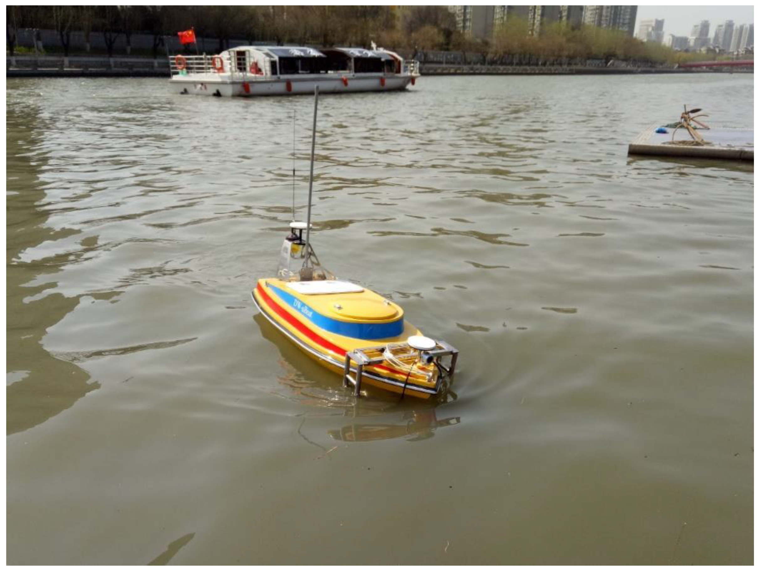
2.1. DW-uBoat USV

DW-uBoat, developed independently by the Institute of Marine Vehicle and Underwater Technology in Nanjing, Jiangsu Province, is a small, unmanned surface vehicle with twin propellers installed symmetrically. In this paper, DW-uBoat was used as a test platform to carry out the full-scale test of the USV in a real environment to provide data for the follow-up identification and modeling. The navigation of the DW-uBoat is shown in Figure 1 and its main physical characteristics are listed in

Table 1. DW-uBoat’s physical characteristics.

Parameters	Value
Length overall	1.80	m
Breadth	0.70	m
Draft	0.24	m
Displacement	75	kg
Propeller diameter	14	cm
Distance between two propellers	29	cm
Max propeller revolution rate	1200	Rpm
Endurance	12	h

.

The DW-uBoat consists of three parts: a hull, dynamic propulsion system, and functional modules. It uses two servo electrical motors to impel twin propellers to move in the scheme of its dynamic propulsion system. Because it is not equipped with a rudder or propeller, the DW-uBoat relies on two thrusters revolving at different speeds to control its course. Two thrusters operating at the same rate of revolution keep the USV in a straight line in theory. The system of functional modules is equipped with various sensors, such as high-definition cameras, a global positioning system, and compass. The main components of the DW-uBoat USV are listed in

Table 2. Parameters of DW-uBoat USV.

Parameters	Content	Characteristics
System of communication	VHF Wireless	2.5 km distance
Image transmission	Wireless digital data link
Inertial sensor	SBG Ellipse-A
Motor	Servo integrated motor	3000 rpm/min, 0.6 Nm
Camera	YTH-IPQ16	IP66 protection
Position system	GPS	(horizontal accuracy, heading accuracy ± 0.1 degrees, pitch/roll accuracy < 1 degree, speed accuracy 0.03 m per second); Electronic compass
Controller board	SCM9022	X86 Atom, Dual core 1.66 g

.

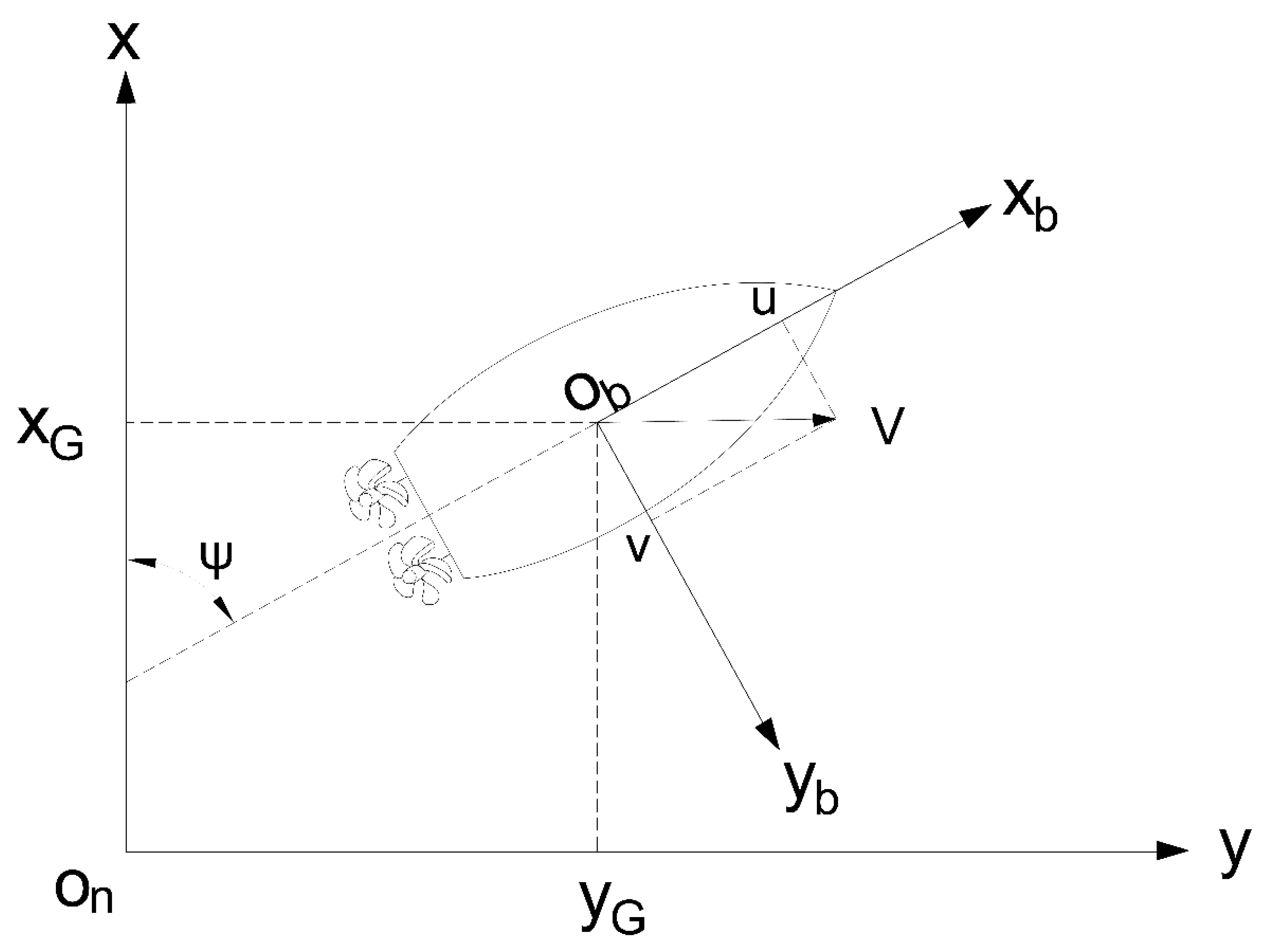
2.2. Kinematics of USV

In general, the movement control system of the USV involves horizontal degrees of freedom, including surge, sway, and yaw [14]. To describe its motion, an inertial frame of reference with origin on and a body-fixed frame of reference with origin O_b were used, as shown in Figure 2. The inertial frame of reference is usually defined as the tangent plane on the surface of the Earth moving with the USV, with the x-axis pointing toward the true north and the y-axis pointing east, different from the directions of the body-fixed axes. The body-fixed frame of reference is a moving coordinate frame that is fixed to the USV. Both frames of reference follow the right-hand thread rule. The position and orientation of the USV are normally described relative to the inertial frame of reference, while the linear and angular velocities should be expressed in the body-fixed frame of reference. In the inertial frame of reference, (x_G, y_G) is the position of the origin O_b that is usually chosen to coincide with a point between ships in the water line, and ψ is the heading angle of the USV. In the body-fixed frame of reference, u, v, and V represent the surge, sway, and total speed of the USV, respectively.

As defined by SNAME, the different quantities above can be expressed in a vectorial setting as follows:

$$\eta =\left[\begin{array}{c}x\\ y\\ \psi \end{array}\right]$$

(1)

$$\nu =\left[\begin{array}{c}u\\ v\\ r\end{array}\right]$$

(2)

where η denotes the vectors of position and orientation, and ν denotes the vectors of linear and angular velocity that are decomposed in the body-fixed frame of reference. The transformation of the two vectors from a body-fixed frame to an inertial frame can be represented by means of the rotation matrix R(ψ), which is expressed as follows:

$$\dot{\eta }=R(\psi )\nu$$

(3)

$$R(\psi )=\left[\begin{array}{ccc}\cos \psi & -\sin \psi & 0\\ \sin \psi & \cos \psi & 0\\ 0& 0& 1\end{array}\right]$$

(4)

2.3. Dynamic Model of USV

The rigid-body kinetics of the USV in surge, sway, and yaw motions can be derived by applying the Newtonian formulation, which can be expressed as:

$$\{\begin{array}{l}(m+m_x)\dot{u}-(m+m_y)rv=X_H+X_P\\ (m+m_x)\dot{v}+(m+m_y)ru=Y_H+Y_P\\ (I_Z+J_Z)\dot{r}=N_H+N_P\end{array}$$

(5)

where m is the mass of the ship, m_x and m_y are the added masses, I_z is the moment of inertia about the z-axis, J_z is the additional inertia, u, v, and r are the speeds of surge and sway, and the yaw rate, respectively, X_H, Y_H, and N_H are the viscous hydrodynamic forces/moments, and X_P, Y_P, N_P are the thrusts/torques of the propeller.

As the DW-uBoat is not equipped with a side thruster and there are no active swaying forces, the sway could only be generated by Coriolis–centripetal forces due to the rotation of the body-fixed frame relative to the inertial frame of reference. However, a coupling was found between the v- and r-related hydrodynamic coefficients. Furthermore, v is small, and the effects of higher-order terms are not considered in this paper. We simplified Inoue’s model [15] to obtain the following computational model of viscous hydrodynamic forces and moments:

$$\{\begin{array}{c}{X}_H=X_{uu}{u}^2+X_{rr}{r}^2\\ Y_H=Y_{v}v+Y_{r}r+Y_{\left|r\right|r}\left|r\right|r\\ N_H=N_{v}v+N_{r}r+N_{\left|r\right|r}\left|r\right|r\end{array}$$

(6)

where $X_{uu},X_{rr},Y_v,Y_r,Y_{\left|r\right|r},N_v,N_r,N_{\left|r\right|r}$ are the hydrodynamic coefficients.

The thrust of the propellers is the exclusive active source of force of the DW-uBoat, and can be generated by controlling the speed of the motors to keep the USV moving forward against external resistance. Woo et al. (Ref. [16]) described the thrust and torque as follows:

$$\{\begin{array}{c}{X}_P=(T_s+T_p)\\ Y_P=0\\ N_P=(T_p-T_s)l/2\end{array}$$

(7)

where T_s and T_p denote the thruster forces of the starboard-side thruster and the port-side thruster, respectively, and l is the beam of the DW-uBoat.

The thruster force can be described as a function of the rate of revolution of the propeller and its diameter, and is expressed as follows:

$$T=(1-t)k\rho n^2{D}^4$$

(8)

where t is the deduction coefficient of the thrust, k is the thrust coefficient, ρ is the density of water, n is the input rate of revolution, and D is the diameter of the propeller.

3. MK-SVR Algorithm for Modeling and Identification

3.1. SVR Formulation

The SVM is a statistical method based on supervised learning that was proposed in the 1990s [9]. The objective of the SVM is to obtain the equation of the hyperplane of structural risk minimization. In the context of regression, the SVM is called the SVR. For the training data {(x_i,y_i), i = 1, 2, … N}, where $x_i\in R^n$ is the input data, $y_i\in R$ is the target value for x_i and N is the number of training samples. The SVR equation of the hyperplane is presented as:

$$f(x)={\omega }^{T}x+b$$

(9)

where ω denotes the matrix of weights and b denotes the bias constant.

In contrast to traditional regression algorithms, SVR enables the maximum deviation ε between f(x) and y_i. The value of the loss function $l_{\epsilon }$ is chosen according to the following formula:

$$l_{\epsilon }=\{\begin{array}{cc}0,& if\left|f(x_i)-y_i\right|<\epsilon \\ \left|f(x_i)-y_i\right|-\epsilon ,& otherwise\end{array}$$

(10)

Therefore, the equation of the hyperplane can be obtained by minimizing the optimization problem as follows:

$$\underset{\omega ,b}{\min }\frac{1}{2}{\Vert \omega \Vert }^2+C{\displaystyle \sum _{i=1}^N{l}_{\epsilon }}(f(x_i)-y_i)$$

(11)

where C is the regularization parameter.

Slack variables ${\xi }_i$ and ${\hat{\xi }}_i$ were selected to make the model more robust so that it can handle unfeasible constraints of the optimization problem as follows:

$$\begin{array}{l}\underset{\omega ,b,{\xi }_i,{\hat{\xi }}_i}{\min }\frac{1}{2}{\Vert \omega \Vert }^2+C{\displaystyle \sum _{i=1}^N({\xi }_i+{\hat{\xi }}_i)}\\ \begin{array}{cc}s.t.& \begin{array}{c}f(x_i)-y_i\le \epsilon +{\xi }_i\\ y_i-f(x_i)\le \epsilon +{\hat{\xi }}_i\\ {\xi }_i\ge 0,{\hat{\xi }}_i\ge 0,i=1,2,\dots ,N\end{array}\end{array}\end{array}$$

(12)

The optimal solution can be obtained by solving the dual form of Equation (7). The Lagrange multipliers were imposed to solve this problem:

$$\begin{array}{l}L(\omega ,b,\alpha ,\hat{\alpha },\xi ,\hat{\xi },\mu ,\hat{\mu })=\frac{1}{2}{\Vert \omega \Vert }^2+C{\displaystyle \sum _{i=1}^N({\xi }_i+{\hat{\xi }}_i)}-{\displaystyle \sum _{i=1}^N{\mu }_i{\xi }_i}-{\displaystyle \sum _{i=1}^N{\hat{\mu }}_i{\hat{\xi }}_i}\\ +{\displaystyle \sum _{i=1}^N{\alpha }_i(f(x_i)-y_i-\epsilon -{\xi }_i)+{\displaystyle \sum _{i=1}^N{\hat{\alpha }}_i(y_i-f(x_i)-\epsilon -{\hat{\xi }}_i)}}\end{array}$$

(13)

where ${\mu }_i\ge 0,{\hat{\mu }}_i\ge 0,\alpha \ge 0,\hat{\alpha }\ge 0$.

We then computed the derivatives of ω, b, e_i, and α_i, and set them to zero to obtain the following:

$$\{\begin{array}{c}\omega ={\displaystyle \sum _{i=1}^N({\hat{\alpha }}_i-{\alpha }_i)x_i}\\ 0={\displaystyle \sum _{i=1}^N({\hat{\alpha }}_i-{\alpha }_i)}\\ C={\alpha }_i+{\mu }_i\\ C={\hat{\alpha }}_i+{\hat{\mu }}_i\end{array}$$

(14)

By placing Equation (9) into the Lagrangian function, the dual problem can be expressed as follows:

$$\begin{array}{l}\underset{\alpha ,\hat{\alpha }}{\max }{\displaystyle \sum _{i=1}^N{y}_i({\hat{\alpha }}_i-{\alpha }_i)}-\epsilon ({\hat{\alpha }}_i+{\alpha }_i)-\frac{1}{2}{\displaystyle \sum _{i=1}^N{\displaystyle \sum _{j=1}^N({\hat{\alpha }}_i-{\alpha }_i)}}({\hat{\alpha }}_j-{\alpha }_j)x_i^T{x}_j\\ \begin{array}{cc}s.t.& \begin{array}{c}{\displaystyle \sum _{i=1}^N({\hat{\alpha }}_i-{\alpha }_i)=0}\\ 0\le {\hat{\alpha }}_i,{\alpha }_i\le C\end{array}\end{array}\end{array}$$

(15)

Equation (10) meets the Karush–Kuhn–Tucker conditions as follows:

$$\{\begin{array}{c}{\alpha }_i(f(x_i)-y_i-\epsilon -{\xi }_i)=0\\ {\hat{\alpha }}_i(y_i-f(x_i)-\epsilon -{\hat{\xi }}_i)=0\\ {\alpha }_i{\hat{\alpha }}_i=0,{\xi }_i{\hat{\xi }}_i=0\\ (C-{\alpha }_i){\xi }_i=0,(C-{\hat{\alpha }}_i){\hat{\xi }}_i=0\end{array}$$

(16)

The following solution can be acquired by calculating the dual problem:

$$f(x)={\displaystyle \sum _{i=1}^N({\hat{\alpha }}_i-{\alpha }_i)x^T{x}_i}+b$$

(17)

3.2. MK Function and Choosing the Weight Coefficients

The use of the kernel function is typically a simple way to avoid the problem of dimensionality, and is used to compute the inner product caused by the nonlinear transformation of the input space of mapping into a high-dimensional feature space to solve a nonlinear problem [17]. It can be expressed as follows:

$$K(x,x_i)=\varphi {(x)}^T\varphi (x_i)$$

(18)

where φ(x) is the transformation of mapping x into a high-dimensional feature space.

The solution can be rewritten as follows for the nonlinear problem:

$$f(x)={\displaystyle \sum _{i=1}^N({\hat{\alpha }}_i-{\alpha }_i)K(x,x_i)}+b$$

(19)

The kernel function can be used in a variety of forms, each with its own characteristics, and the SVRs constructed using each have different characteristics. In general, they can be classified into two distinct types: the global kernel function and the local kernel function. The former has good generalization ability for mastering global information far from the test points, while the latter has a better learning ability owing to its higher sensitivity to the features of samples with narrow distributions. The polynomial kernel (PK), the prominent representative of the global kernel function and the radial basis function (RBF), is a representative local kernel function that can be selected and calculated as shown in Equations (20) and (21), respectively:

$$K{(x,x_i)}_d={(g\cdot x^T{x}_i+c0)}^d$$

(20)

$$K{(x,x_i)}_{RBF}=\exp (-\gamma {\Vert x-x_i\Vert }^2)$$

(21)

Based on Mercer’s theorem (1909), the appropriate conditions for a kernel function can be described as follows:

Let X be a compact subset of Rⁿ and K be a continuous and symmetric function; there is a integral operator $T_k:L_2(X)\to L_2(X)$ that makes $(T_{k}f)(\cdot )={\displaystyle \underset{X}{\int }K(\cdot ,x)}f(x)dx$ positive. The above would be expressed as follows:

$${\displaystyle \underset{X\times X}{\int }K(x,z)f(x)f(z)dxdz\ge 0\begin{array}{cc}& \forall f\in L_2(X)\end{array}}$$

(22)

After expanding $K(x,z)$ to a sequence of the consequent $T_k$ characteristic function ${\varphi }_j\in L_2(\chi )$ and normalization, we can obtain ${\Vert {\varphi }_j\Vert }_{L_2}=1,{\lambda }_j\ge 0$ and the following relation:

$$K(x,z)={\displaystyle \sum _{i=1}^n{\lambda }_j}{\varphi }_j(x){\varphi }_j(z)$$

(23)

We took $\Phi (x)$ as ${(\sqrt{{\lambda }_1}{\varphi }_1(x),\sqrt{{\lambda }_2}{\varphi }_2(x),\dots ,\sqrt{{\lambda }_n}{\varphi }_n(x))}^T$ and obtained the kernel function below:

$$K(x,z)=<\Phi (x),\Phi (z)>$$

(24)

Based on the above, we know that if the matrix defined by a function in an arbitrary finite point set of Rⁿ is semi-positive, the fuction can be a kernel fuction. The convex combination of common kernel functions is an important means of constructing the MK. In this paper, an MK constructor is developed by combining the PK and RBF:

$$K(x,x_i)={\exp }^{-{\sigma }^2}K{(x,x_i)}_d+(1-{\exp }^{-{\sigma }^2})K{(x,x_i)}_{RBF}$$

(25)

where ${\exp }^{-{\sigma }^2}$ and $(1-{\exp }^{-{\sigma }^2})$ are the weights of the PK and the RBF, respectively.

With an arbitrary vector, we can obtain ${\alpha }^{\prime }K{(x,x_i)}_d\alpha \ge 0;{\alpha }^{\prime }K{(x,x_i)}_{RBF}\alpha \ge 0$. Furthermore, the validity of MK can be described as follows:

$${\alpha }^{\prime }({\exp }^{-{\sigma }^2}K{(x,x_i)}_d+(1-{\exp }^{-{\sigma }^2})K{(x,x_i)}_{RBF})\alpha ={\exp }^{-{\sigma }^2}{\alpha }^{\prime }K{(x,x_i)}_d\alpha +(1-{\exp }^{-{\sigma }^2}){\alpha }^{\prime }K{(x,x_i)}_{RBF}\alpha \ge 0$$

(26)

So, the convex combination of the PK and RBF can be used as the kernel function. In case $1\ge {\exp }^{-{\sigma }^2}\ge 0$, the problems of low precision and poor generalization due to either the PK or the RBF can be avoided.

To implement adaptive adjustment, the coefficients of the convex combination of the MK functions need to be optimized. K-fold cross-validation (K-fold CV) is used to find the ideal solution; the larger the value of K is, the greater is the number of folds, which can reduce error. However, the larger the training set is, the greater the variance and the time cost. Therefore, five-fold CV was used to select a suitable weight coefficient in the MK function. The samples were divided randomly into five groups of equal size. A single subset was retained as the data for validation while the other four subsets were used for training. The cross-validation was repeated five times, and each subset was verified once. The mean squared error of the five groups was regarded as the final error value, and the parameter with the least error was chosen as the weight coefficient.

3.3. Identification and Modeling

Using the field data of DW-uBoat USV as the change data sequence of the system input and output, the support vector regression (MK-SVR) method based on the mixed kernel function was proposed to identify the dynamics model of DW-uBoat USV to realize the manipulation motion prediction and evaluate the prediction effect.

The processes of identification and modeling based on the MK-SVR method are shown schematically in Figure 3. The steps are as follows:

(1)

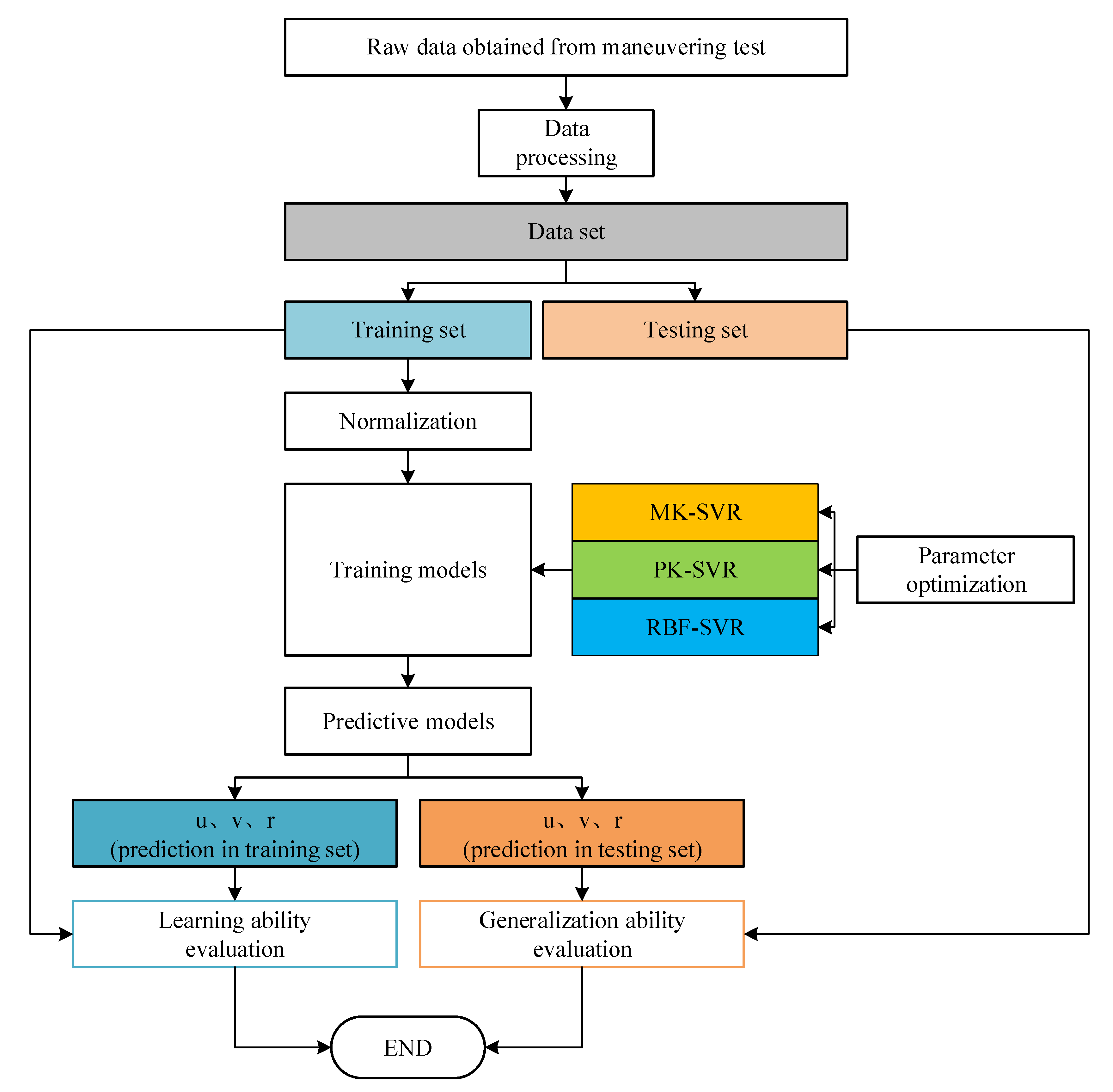
The samples for system identification obtained from the maneuvering test were divided into a training set and a verification set.

(2)

The training data were taken as the input for system identification after being normalized.

(3)

The CV method was used to seek the optimum parameters in the SVR and the weight in the MK function.

(4)

Training and prediction models were established for PK-SVR, RBF-SVR, and MK-SVR.

(5)

The models were used to predict the surge velocity, sway velocity, and the yaw rate, and their results were compared.

4. Zig-Zag Test and Data Processing

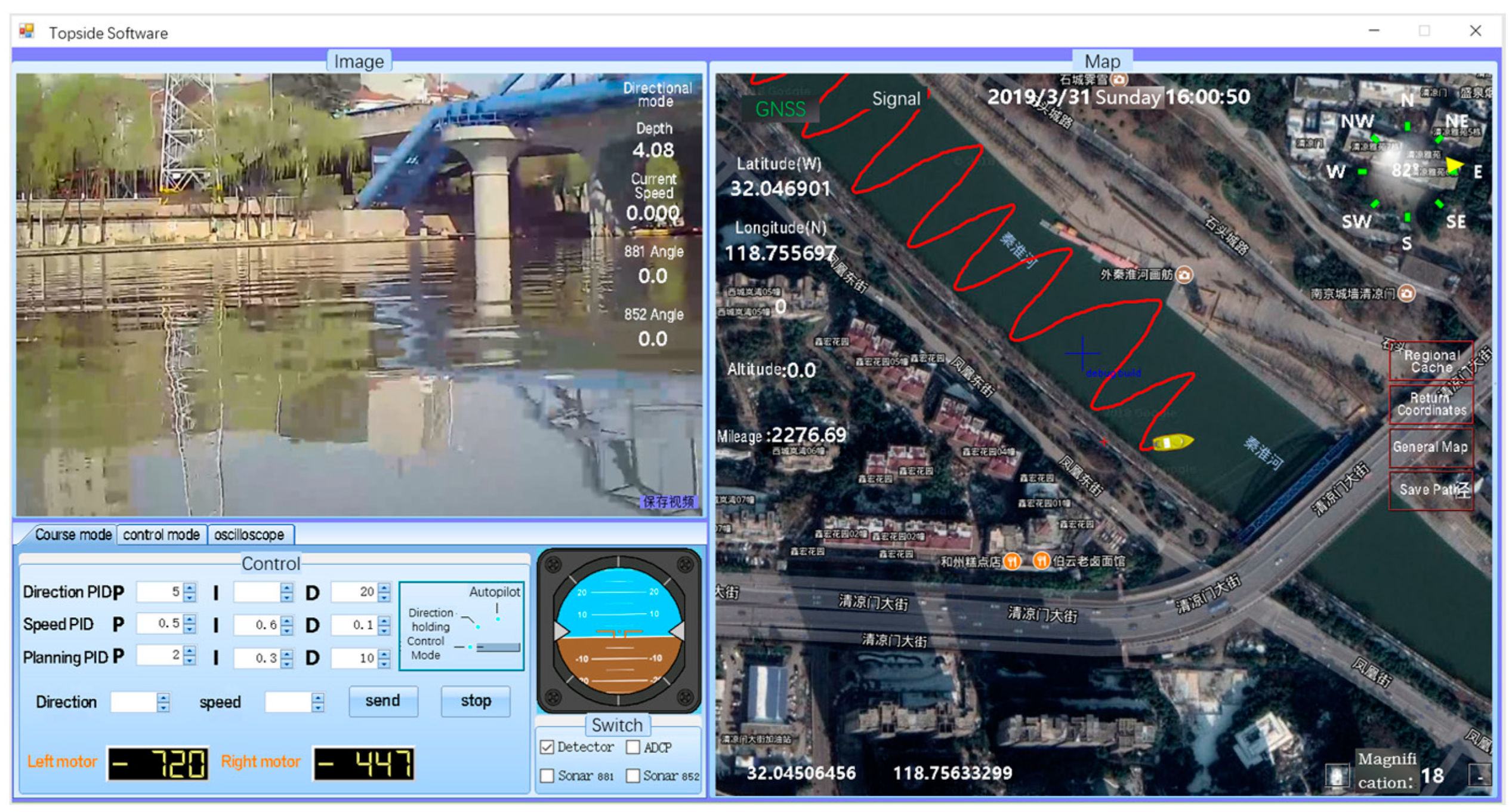
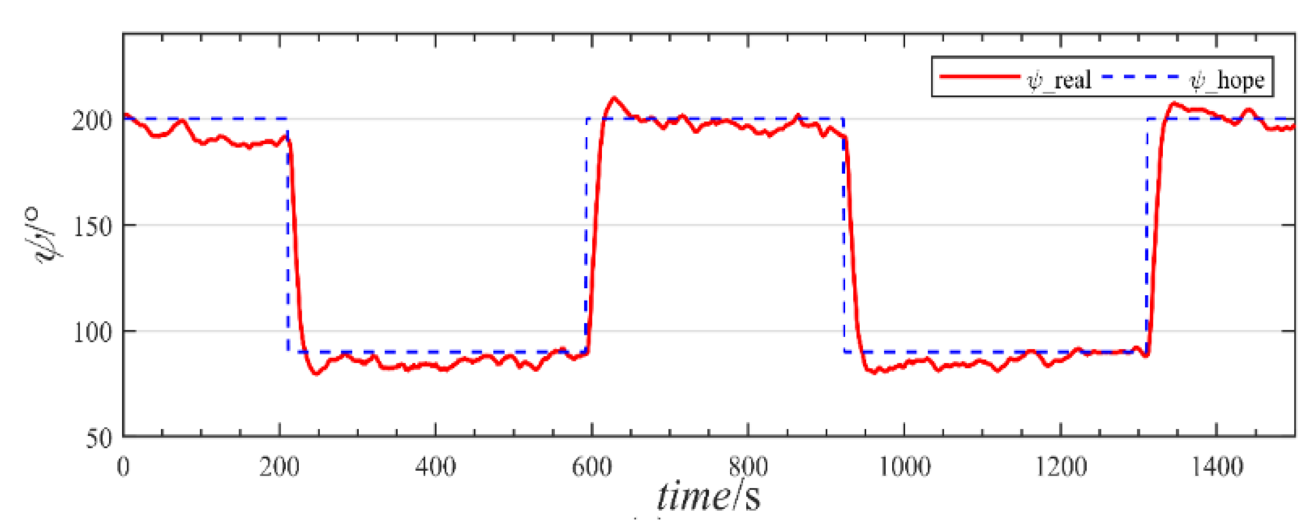
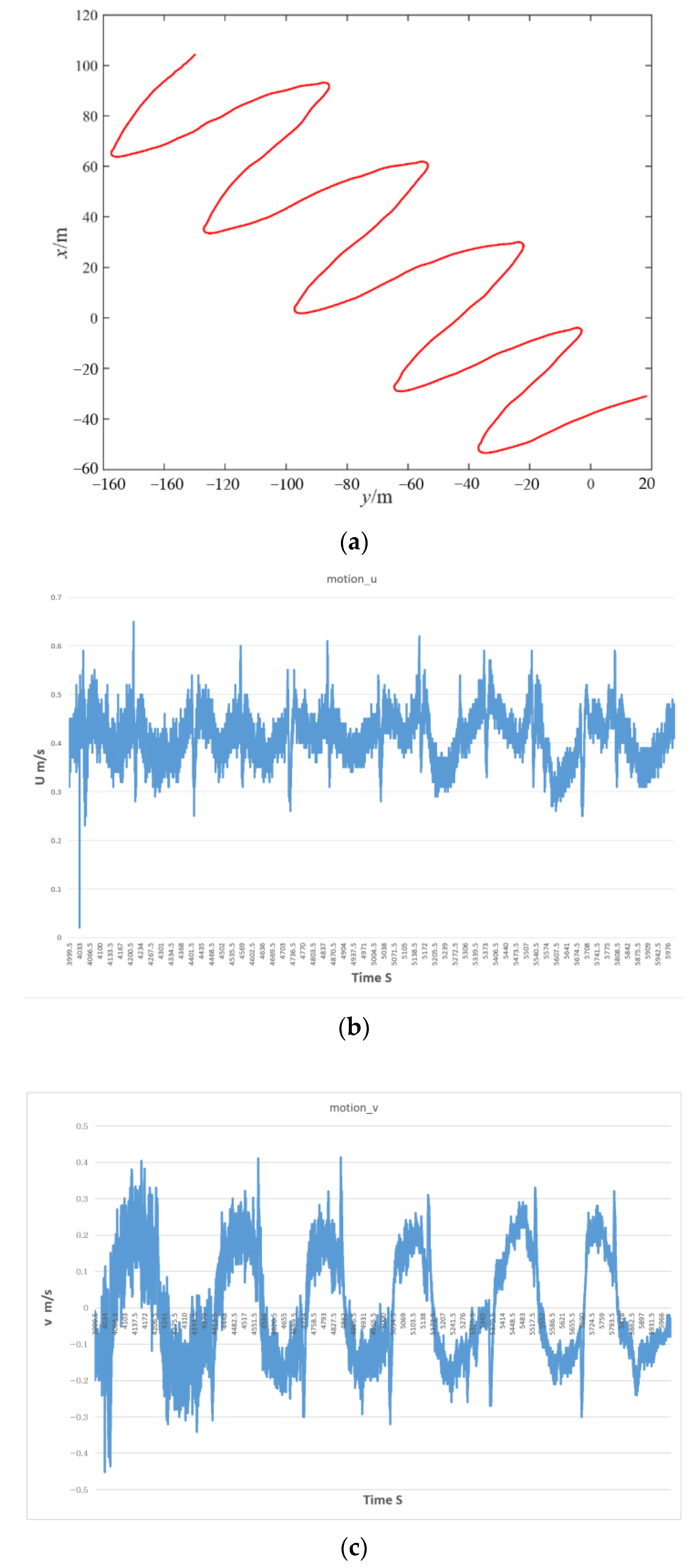
4.1. Zig-Zag Test of USV

The maneuverability of a ship is defined as its ability to maintain or change its motion according to the intention of the operator. The zig-zag test reflects a ship’s steering performance and directional stability, and can thus be used to obtain sample data for follow-up work related to modeling-based identification.

The DW-uBoat use a PC104 computer with RTOS to process data from sensors and control the motion. Both remote control and automatic driving modes are used. The software on the remote computer is developed by .Net Framework. The navigation is based on Gmap.net components. For automatic driving, firstly, the destination points were set; secondly, the LOS algorithm automatically output the desired commands to the PID controller; finally, the PID controller offered corresponding thruster orders.

The full-scale test of the USV was carried out in Stone City along Qinhuai River. The trajectory tracking control relied on a controller developed by the Institute of Marine Vehicle and Underwater Technology [13], and the monitoring interface of the upper computer is shown in Figure 4. The software is used for control and navigation. The test data, including the coordinates $(x,y)$, heading angle ψ, surge, and sway of the DW-uBoat as well as the speed of the motor, were monitored in real time by using sensors and stored every 0.25 s. Figure 5 shows the expected and raw values of the heading angle, and Figure 6 shows the raw motion trajectory in the testing process.

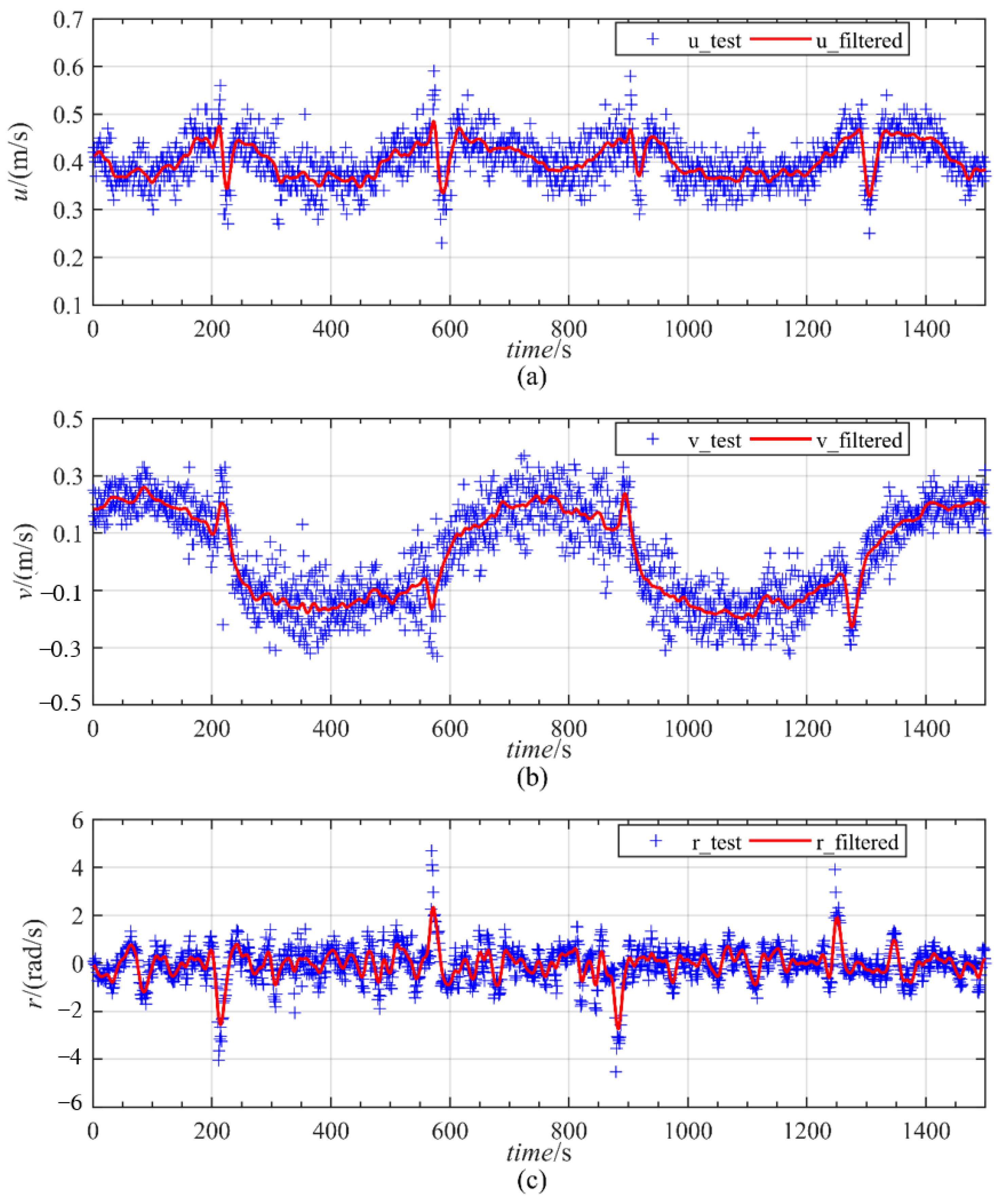
4.2. Data Processing

The test was carried out in a channelized urban river that was approximately 70 m wide and 1–7 m deep, which met the requirements of the maneuvering test. The flow was relatively stable and featured prominent waves and currents throughout the test, which means that the measured data included the flow velocity and other noise that needed to be removed before the data could be used as the input to the algorithm. The Gaussian filtering method was used to remove noise, and the datasets before and after filtering are shown in Figure 7. The sub-figures denote the surge and sway velocities as well as the yaw rate of the DW-uBoat. It is clear that when the yaw angle changed, the surge and sway velocities, and the yaw rate underwent significant changes. Fluctuations were observed in the test data for the USV with a shallow draft. This was caused by the persistent yawing motion of the USV to maintain its course against disturbances due to the current and the large randomness of external interference, which made it difficult to ensure that the curves were smooth even after filtering.

Even if the direction of flow was known, the surge and sway velocities were differently influenced by the flow velocity for the two heading angles, and the relative speed of water could be calculated by using the following formula:

$$\{\begin{array}{c}u=uc-V_c\cos (\theta -\psi )\\ v=vc-V_c\sin (\theta -\psi )\end{array}$$

(27)

where uc and vc represent the surge and sway velocities with respect to the ground, respectively, V_c denotes the flow velocity, and θ is the angle of flow in the inertial coordinate system.

Assuming that the flow was steady, the surge and sway velocities relative to water were calculated and are shown in Figure 8. The surge velocity with respect to the ground fluctuated around 0.4 m/s owing to being in the fixed speed mode, and the surge velocity relative to water was greater than 0.4 m/s when navigating upstream. In addition, the directions of the sway velocity with respect to the ground were different at the two heading angles due to the influence of flow, which also shows that the sway velocity of the USV relative to water was close to zero.

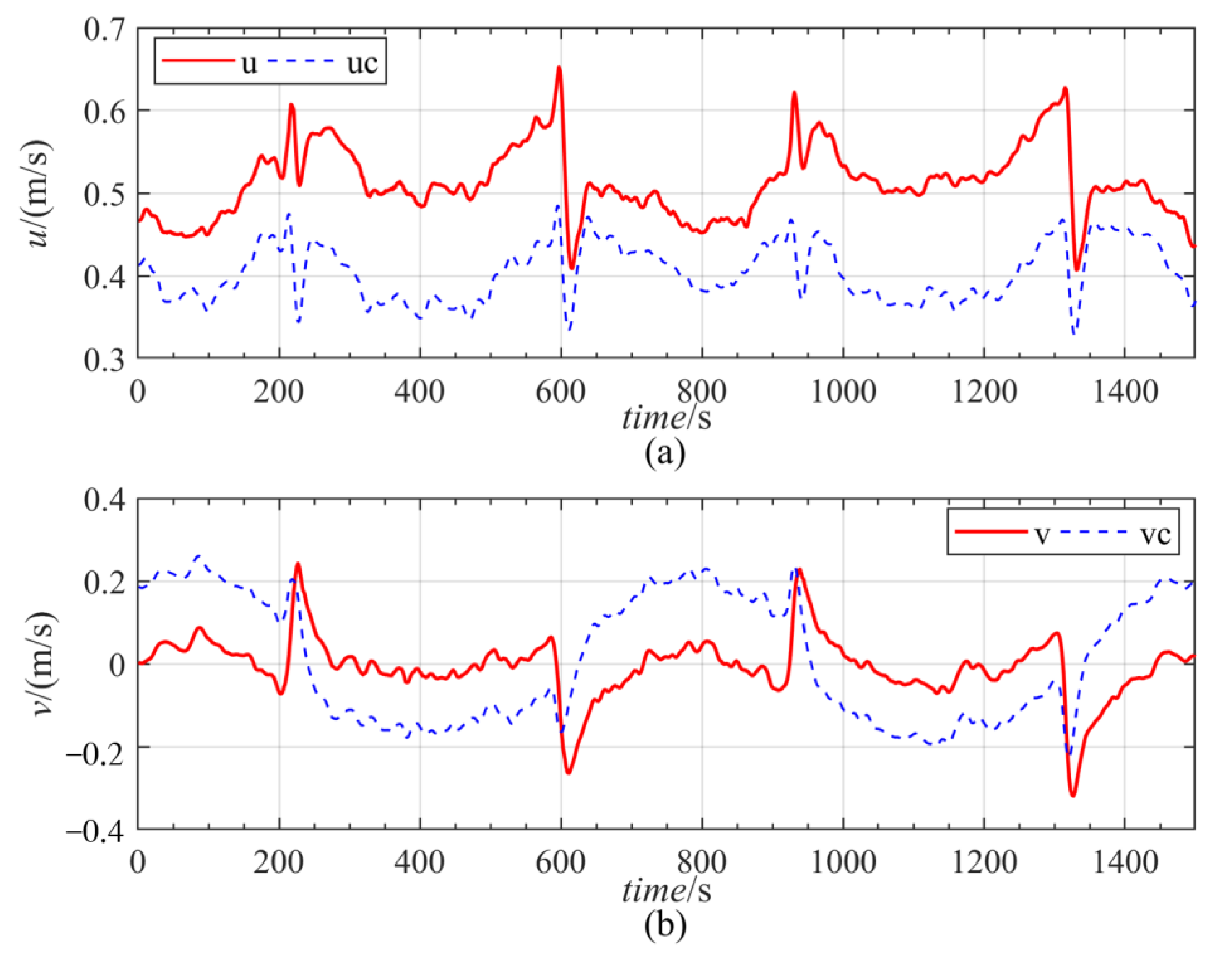
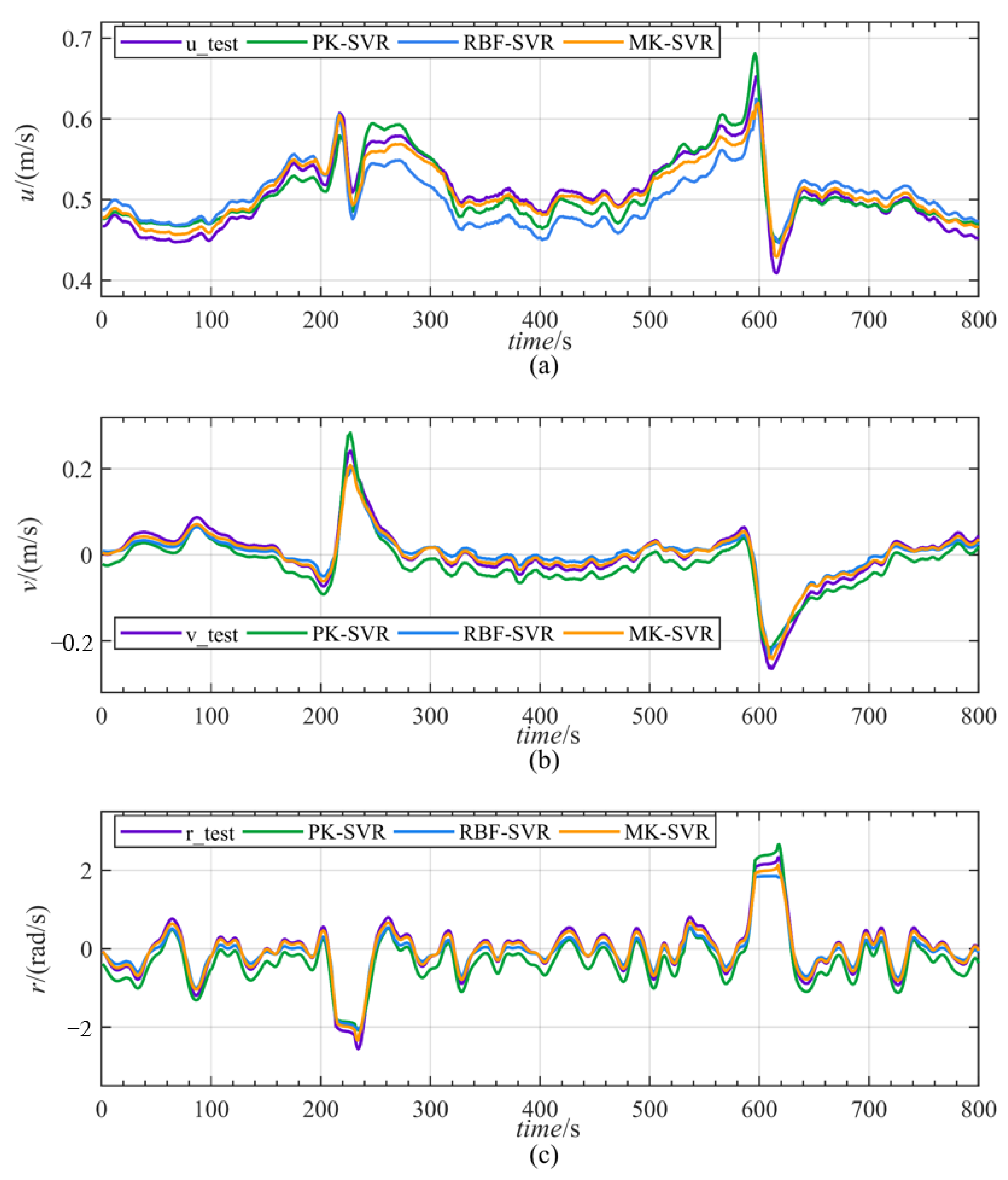
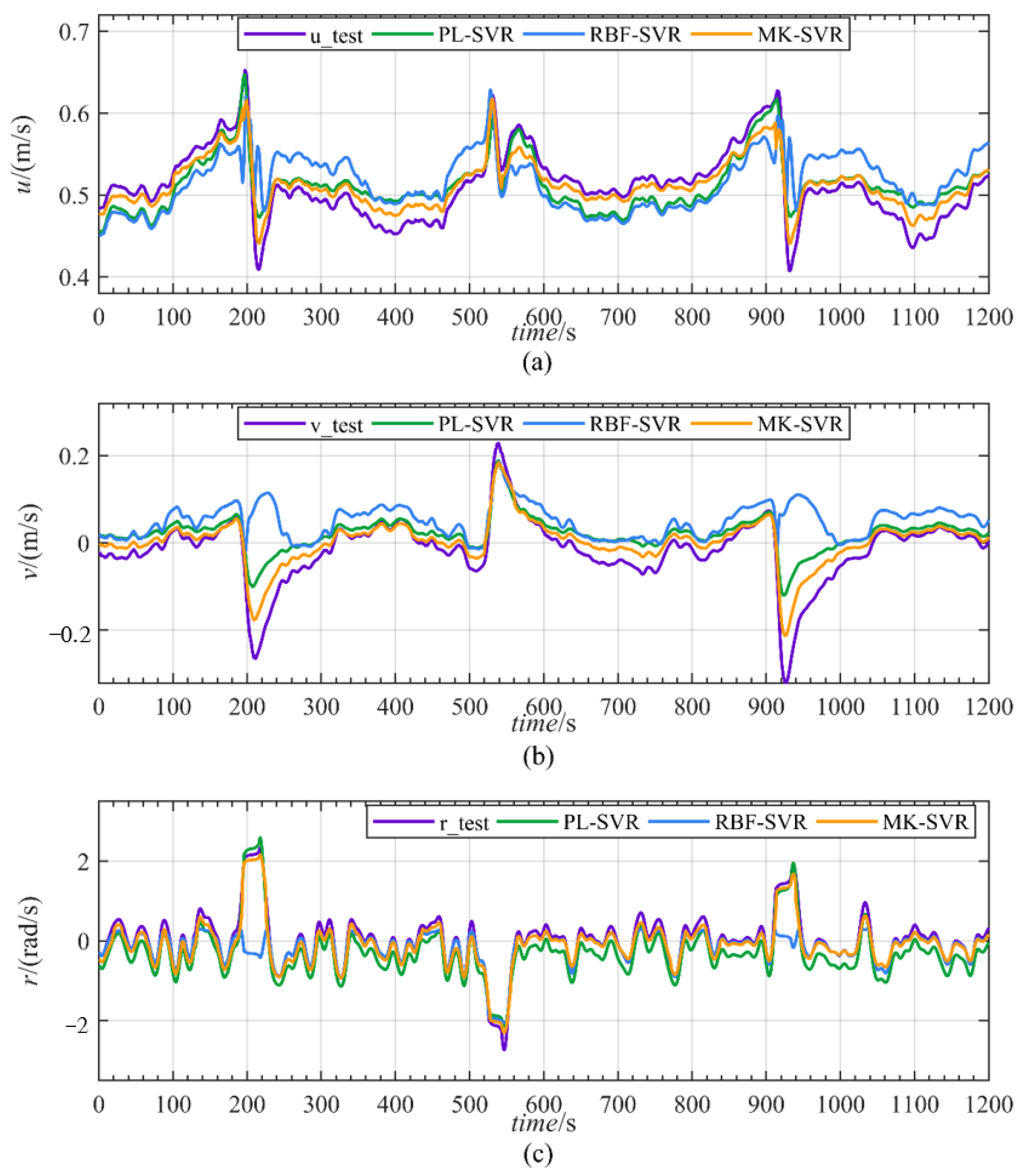
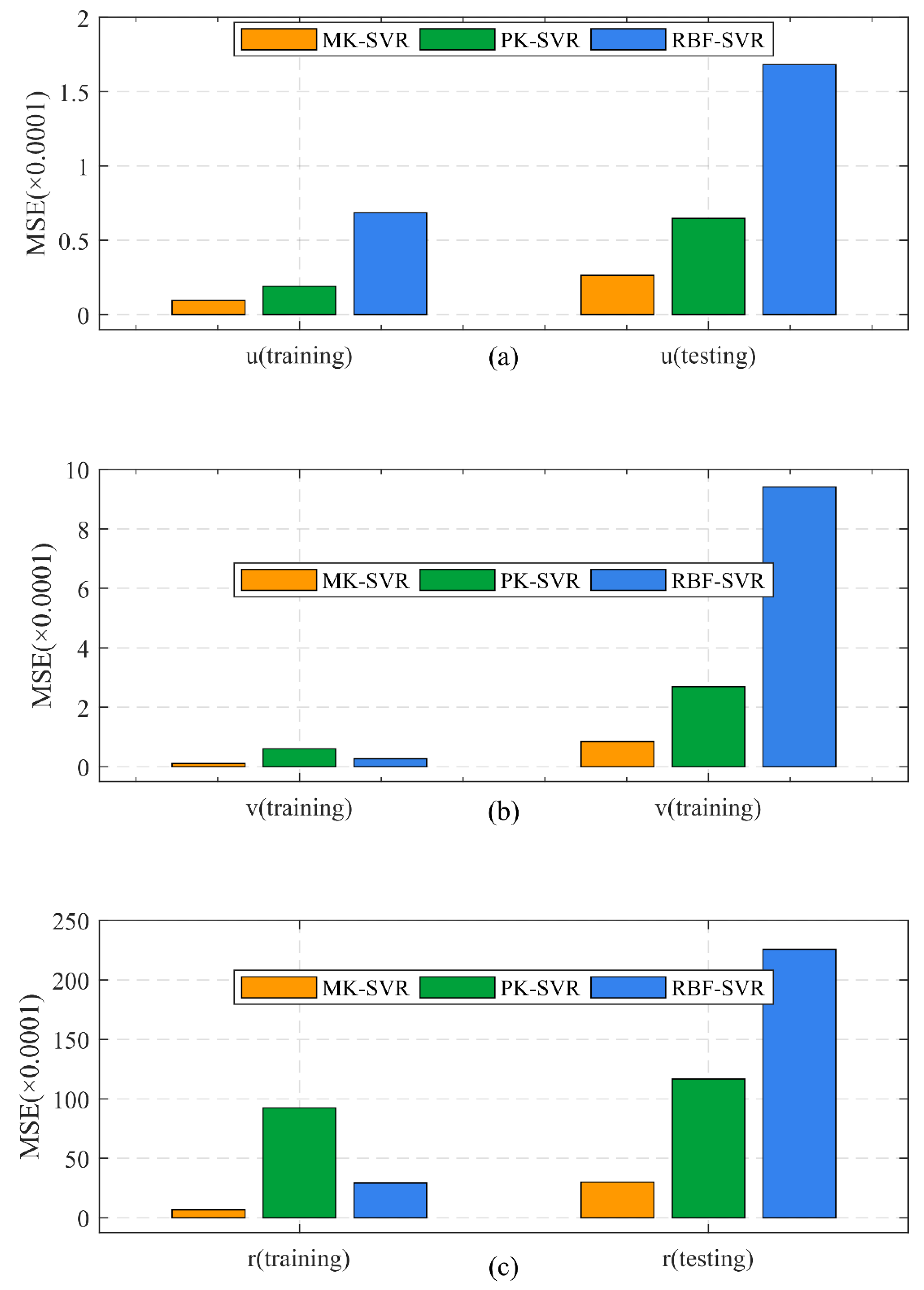
5. Comparison of the Results of Prediction

The model established in Section 2 and the data detailed in Section 3 were used to identify and model the motion of ships, and the good performance of the MK-SVR method was verified by comparing it with SVR based on a single PK function and the RBF kernel. We used samples acquired within 800 s as the training dataset and those acquired within 1200 s as the verification dataset. The MSE was used as the index to assess the accuracy of the prediction models.

Figure 9 illustrates the predicted and the actual data on the surge velocity, sway velocity, and yaw rate. This shows that all three methods had good learning ability. MK-SVR was significantly better at predicting the surge velocity than the other two methods. MK-SVR and RBF-SVR performed similarly in terms of predicting the sway velocity and the yaw rate, whereas PK-SVR had the poorest performance in terms of agreement with the test data.

Comparisons of the surge velocity, sway velocity, and yaw rate predicted by the three methods on the validation set are shown in Figure 10. It is clear that MK-SVR and PK-SVR were significantly superior to RBF-SVR in terms of predicting the surge velocity, and the trend of changes in their curves as predicted by MK-SVR was more similar to that of the experimental data than the trend predicted by PK-SVR. Both MK-SVR and PK-SVR exhibited good predictive capability for the sway velocity and the yaw rate, but MK-SVR was slightly more accurate, as reflected by the MSE values. RBF-SVR failed to accurately predict these factors in some intervals, and on occasion even predicted a trend opposite to the actual trend. It is worth mentioning that Xu et al. [6], conducted a contrastive study of SVR with a single kernel function and neural network method. From the results of this paper, SVM based on the single kernel function showed a better ability of identification than the neural network method, which has a higher accuracy and faster convergence speed when predicting the motion of USV, verified by the full-scale test. That is, MK-SVR has prominent advantages for predicting the maneuvering motion of USV in a real environment.

The MSE index in Figure 11 shows that the predictive accuracies of all three methods were lower in the validation set than the training set, but the MK-SVR method still delivered a satisfactory MSE index of less than 0.05 in a practical environment. Moreover, relatively large deviations were observed in the predicated sway velocity and yaw rate, possibly because their values fluctuated less than in the case of a sudden change in course. When a large amount of noise made it difficult to distinguish the dynamic characteristics of the USV, the problem of over-fitting occurred.

Table 3. Comparison of CPU times of the three methods in training set and testing set.

		MK-SVR	PK-SVR	RBF-SVR
In training set	Surge velocity	36 s	37 s	34 s
	Sway velocity	41 s	44 s	38 s
	Yaw rate	40 s	41 s	38 s
In testing set	Surge velocity	42 s	40 s	43 s
	Sway velocity	44 s	43 s	46 s
	Yaw rate	42 s	41 s	43 s

shows that the MK-SVR improved the prediction accuracy with the same amount of computational time.

To sum up, the proposed method not only alleviates the problem of features being easily influenced by noise or occlusion to obtain a satisfactory fit with the empirical data, but also restrains local fluctuations in the predicted output due to the RBF kernel. Therefore, the MK-SVR method can be used to formulate dynamic models of USVs using a finite number of samples because it is better in terms of learning and generalization than SVR with a single PK and an RBF kernel.

6. Conclusions

To control the motion of a USV in light of the dual requirements of high precision and generalization, this paper proposed an MK-SVR-based method of identification to establish a model to predict its motion. We focused on the model design, maneuverability test, and data processing. We use DW-uBoat’s raw data as the training and testing datasets for the method.

The proposed identification model was compared with models prevalent in the literature. The main contributions of this study are as follows:

(1)

A full-scale USV test was carried out, and the data obtained from it were used to validate the accuracy of the MK-SVR method in terms of predicting the motion of the USV in an empirical setting.

(2)

Cross-validation was used to automatically search for the best weights in the MK function to better leverage the benefits of the global and local kernels. This helps maintain the accuracy of prediction through adaptive adjustment and reduces the time required for tuning.

(3)

The MK-SVR method was proposed to model and identify the motion of the DW-uBoat USV. The results of experiments showed that the MK-SVR method integrates the advantages of the local and global kernel functions such that it makes more accurate predictions and has better generalization ability than SVR based on the nuclear kernel function. The superior predictive performance of the MK-SVR method is quantified in Table 3 and Figure 7, Figure 8 and Figure 9, with less than 0.05 MSE in a practical environment in DW-uBoat field data.

Based on the SVR algorithm, this study proposes a novel method of dynamics identification for USV, and although some results have been achieved, there are still some works to be further studied.

This study is based on inland river environments with common hydrology factors. In field applications of USVs, their motions are disturbed by complex environmental loads. In the future, we will intend to offshore applications and consider the influence of waves on the hydrodynamics model.

References

1. Qian, Z.; Lu, J.; Sun, X. Brief Analysis of Deep Learning Application in Future Unmanned Surface Vehicle Platform. Ship Build. China 2020, 61, 6–13. [Google Scholar]
2. Rajesh, G.; Bhattacharyya, S.K. System Identification for Nonlinear Maneuvering of Large Tankers Using Artificial Neural Network. Appl. Ocean Res. 2008, 30, 256–263. [Google Scholar] [CrossRef]
3. Pan, C.-Z.; Lai, X.-Z.; Yang, S.X.; Wu, M. An Efficient Neural Network Approach to Tracking Control of an Autonomous Surface Vehicle with Unknown Dynamics. Expert Syst. Appl. 2013, 40, 1629–1635. [Google Scholar] [CrossRef]
4. Luo, W.; Hu, B.; Li, T. Neural Network Based Fin Control for Ship Roll Stabilization with Guaranteed Robustness. Neurocomputing 2017, 230, 210–218. [Google Scholar] [CrossRef]
5. Jiang, Y.; Hou, X.-R.; Wang, X.-G.; Wang, Z.-H.; Yang, Z.-L.; Zou, Z.-J. Identification Modeling and Prediction of Ship Maneuvering Motion Based on LSTM Deep Neural Network. J. Mar. Sci. Technol. 2022, 27, 125–137. [Google Scholar] [CrossRef]
6. Xu, P.-F.; Cheng, C.; Cheng, H.-X.; Shen, Y.-L.; Ding, Y.-X. Identification-Based 3 DOF Model of Unmanned Surface Vehicle Using Support Vector Machines Enhanced by Cuckoo Search Algorithm. Ocean Eng. 2020, 197, 106898. [Google Scholar] [CrossRef]
7. Luo, W.; Zou, Z. Identification of Response Models of Ship Maneuvering Motion Using Support Vector Machines. Available online: https://www.researchgate.net/publication/292425432_Identification_of_response_models_of_ship_maneuvering_motion_using_support_vector_machines (accessed on 13 October 2022).
8. Luo, W.; Zou, Z. Parametric Identification of Ship Maneuvering Models by Using Support Vector Machines. Available online: https://www.researchgate.net/publication/233653524_Parametric_Identification_of_Ship_Maneuvering_Models_by_Using_Support_Vector_Machines (accessed on 13 October 2022).
9. Zhou, B.; Shi, A. Empirical Mode Decomposition Based LSSVM for Ship Motion Prediction; Zhou, B., Shi, A., Zeng, Z., Eds.; Lecture Notes in Computer Science; Springer: Berlin/Heidelberg, Germany, 2013; Volume 7951, ISBN 978-3-642-39064-7. [Google Scholar]
10. Wang, Z.; Zou, Z.; Guedes Soares, C. Identification of Ship Manoeuvring Motion Based on Nu-Support Vector Machine. Ocean Eng. 2019, 183, 270–281. [Google Scholar] [CrossRef]
11. Luo, W.; Guedes Soares, C.; Zou, Z. Parameter Identification of Ship Maneuvering Model Based on Support Vector Machines and Particle Swarm Optimization. J. Offshore Mech. Arct. Eng. 2016, 138, 031101. [Google Scholar] [CrossRef]
12. Zhu, M.; Hahn, A.; Wen, Y.-Q.; Bolles, A. Identification-Based Simplified Model of Large Container Ships Using Support Vector Machines and Artificial Bee Colony Algorithm. Appl. Ocean Res. 2017, 68, 249–261. [Google Scholar] [CrossRef]
13. Xu, P.-F.; Luo, J. Research on Path Tracking of Unmanned Surface Vehicles. Shipbuild. China 2020, 61, 133–142. [Google Scholar]
14. Fossen, T.I. Handbook of Marine Craft Hydrodynamics and Motion Control; John Wiley & Sons: Hoboken, NJ, USA, 2011. [Google Scholar]
15. Ogawa, A.; Kasai, H. On the Mathematical Model of Manoeuvring Motion of Ships. ISP 1978, 25, 306–319. [Google Scholar] [CrossRef]
16. Woo, J.; Park, J.; Yu, C.; Kim, N. Dynamic Model Identification of Unmanned Surface Vehicles Using Deep Learning Network. Appl. Ocean Res. 2018, 78, 123–133. [Google Scholar] [CrossRef]
17. Scholkopf, B.; Burges, C.; Vapnik, V. Extracting Support Data for a Given Task. 6. In Proceedings of the 1st International Conference on Knowledge & Data Mining, Montreal, QC, Canada, 20–21 August 1995; pp. 255–257. [Google Scholar]
Figure 1. DW-uBoat USV.
Jmse 10 01899 g001
Figure 2. Inertial frame of reference and body-fixed frame of reference.
Jmse 10 01899 g002
Figure 3. Flowchart of identification and modeling based on MK-SVR.
Jmse 10 01899 g003
Figure 4. Monitoring interface.
Jmse 10 01899 g004
Figure 5. Heading angle.
Jmse 10 01899 g005
Figure 6. Zig-zag trajectory and original date for u. v. (a) Location coordinate; (b) speed of u; (c) speed of v.
Jmse 10 01899 g006
Figure 7. Partial surge velocities, sway velocities, and yaw rates of the USV before and after filtering. (a) Surge; (b) Sway; (c) Yaw.
Jmse 10 01899 g007
Figure 8. Partial surge and sway velocities relative to the ground and water. (a) Surge; (b) Sway.
Jmse 10 01899 g008
Figure 9. Comparisons of predictions by the three methods using the training data. (a) surge; (b) sway; (c) yaw.
Jmse 10 01899 g009
Figure 10. Comparisons of predictions by the three methods using the test data. (a) Surge velocity; (b) Sway velocity; (c) Yaw.
Jmse 10 01899 g010
Figure 11. Estimated predictive accuracies of the three methods in terms of MSE. (a) Surge MSE (b) Sway MSE; (c) Yaw MSE.
Jmse 10 01899 g011