An Open-Source Benchmark Simulator: Control of a BlueROV2 Underwater Robot

Abstract

This paper presents a simulation model environment for the popular and low-cost remotely operated vehicle (ROV) BlueROV2 implemented in Simulink™ which has been designed and experimentally validated for benchmark control algorithms for underwater vehicles. The BlueROV2 model is based on Fossen’s equations and includes a kinematic model of the vehicle, the hydrodynamics of vehicle and water interaction, a dynamic model of the thrusters, and, lastly, the gravitational/buoyant forces. The hydrodynamic parameters and thruster model have been validated in a test facility. The benchmark model also includes the ocean current, modeled as constant velocity. The tether connecting the ROV to the top-site facility has been modeled using the lumped mass method and is implemented as a force input to the ROV model. At last, to show the usefulness of the benchmark model, a case study is presented where a BlueROV2 is deployed to inspect an offshore monopile structure. The case study uses a sliding mode controller designed for the BlueROV2. The controller fulfills the design criteria defined for the case study by following the provided trajectory with a low error. It is concluded that the simulator establishes a benchmark for future control schemes for position control and trajectory tracking under the influence of environmental disturbances.

1. Introduction

The area of remotely operated vehicles (ROVs) and autonomous underwater vehicles (AUVs) has rapidly developed, with several decades of experience, both in research (see, for example, the study described in [1]) and industrial applications of increasing complexity, both in terms of missions and levels of automation (see for example [2] on cooperative navigation). Regarding the latter, many control algorithms have been proposed, both for simulated and actual vehicles. However, it is generally not immediate to compare control algorithms between them. Indeed, while some articles comparing newly-proposed control laws for ROV stabilization to previous algorithms can easily be found [3,4,5,6,7,8], it is primarily based on simulation models for which the actual physical replica is not easily accessible or affordable, thereby limiting the comparability between control algorithms and the extent of the benchmarking attempt.

More recently, the industry has also evolved towards more affordable products meant for researchers, students, or hobbyists, several of which are proposed under the open-source paradigm (see, for example, OpenROV, OpenROV Trident, BlueROV2) [9]. The advantages of open software and hardware solutions lie in their cost-effectiveness compared to conventional solutions and that they allow increasingly faster development, modifications, and improvements. Among these solutions, the widely-popular BlueROV2 [10] combines an open-source architecture with components of sufficiently good quality, allowing relatively advanced missions (see, for example, [11,12,13]).

Several robot simulators have previously been developed, some of which are specific for underwater robots [14,15,16]. However, the simulators for underwater robots are generally based on a user-defined model, such as the UUV Simulator [14] package for Gazebo or the Simu2VITA [15] block for Simulink™, which makes it challenging to use as a benchmark for control algorithms. Furthermore, these simulators neglect the tether force many underwater robots use for top-site communications or power [17]. The present paper aims at bridging the gap between simulation for control systems and experimental testing by proposing a MATLAB™ and Simulink™ open-source package of the tethered BlueROV2 for the control community as a benchmark in simulation toward full deployment on the same well-known platform. MATLAB™ and Simulink™ have been chosen as they are well-known to the control community and offer various toolboxes to implement advanced control and missions. These missions could be measuring reefs [18], monitoring and removal of marine growth on offshore structures [3,19,20], water quality and ecology monitoring [21], detection of oil plumes [22], fish farm net monitoring [23], etc.

Section 2 will be dedicated to the presentation of the BlueROV2 platform in terms of hardware (frame, thrusters, sensors). In Section 3, we recall the dynamic equations of motions of underwater vehicles propelled by thrusters using the well-known $\mathbf{\eta }$-$\mathbf{\nu }$ Fossen notation [24]. The parameters of this model are then identified for the particular case of the BlueROV2 in Section 4, and the model is then validated using experimental data. Since the tether attached to the ROV has a significant impact on the dynamics, it is included in the overall model, see Section 6. Section 7 proposes a sliding-mode controller meant as a benchmark for the community to compare against subsequent controllers. Section 8 then starts with the presentation of a modular simulator fully implemented in MATLAB™ and Simulink™ and based on the model from Section 3 and the parameters from Section 4. Appendix B provides a detailed guide to using the simulator. Section 9 examines a case study on offshore monopile inspection to demonstrate the use of the proposed simulator. Finally, a few concluding remarks end the paper. The proposed simulator can be found at Github in Supplementary Materials, accessed on 1 October 2022.

2. BlueROV2: An Open-Source Underwater Vehicle

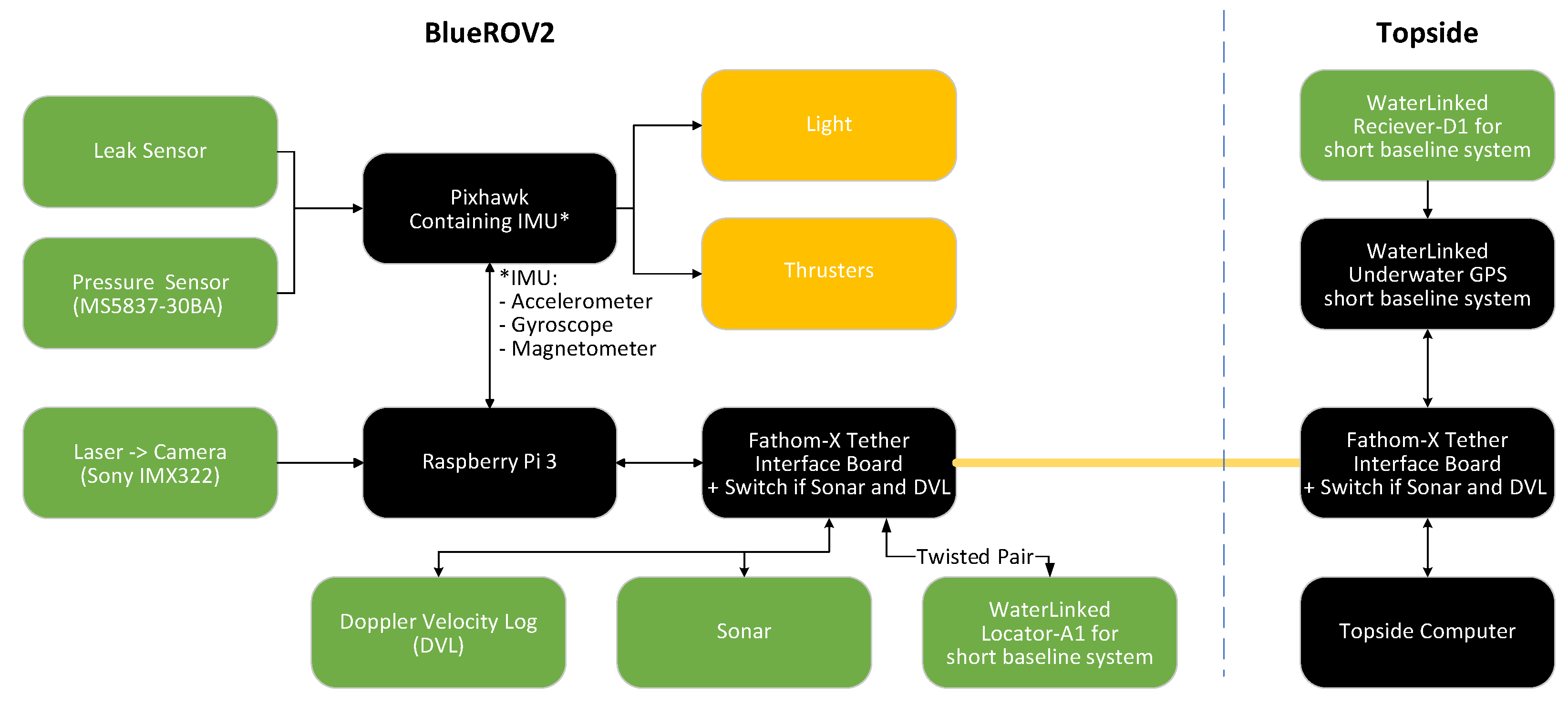
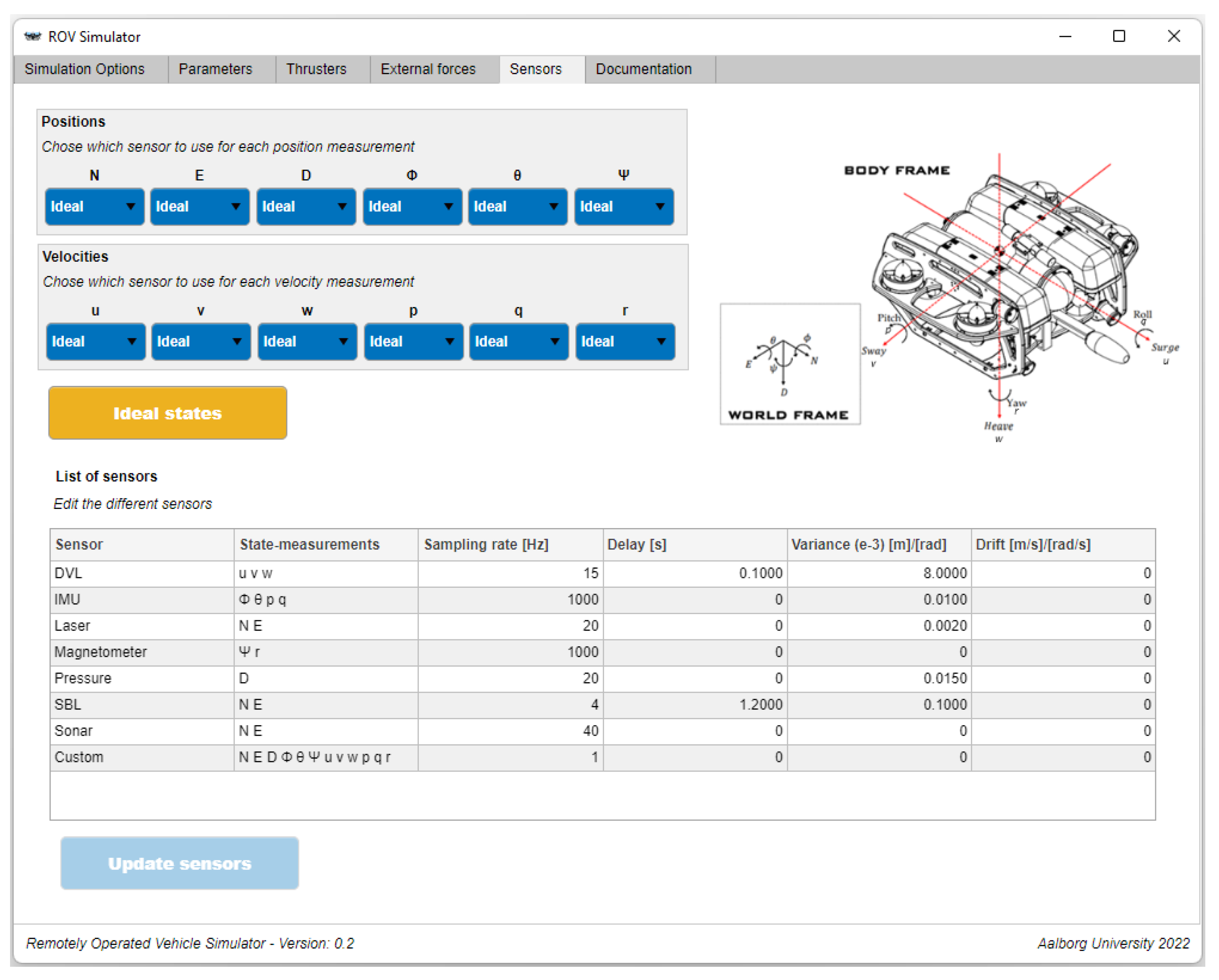
The BlueROV2 is a tethered ROV. The tether is used for communication between the vehicle and a top-side unit. The vehicle can be powered either through the tether or by an onboard battery. The ROV comes with various onboard sensors, including a pressure transmitter, leak detection sensors, a power sense module, an Inertial Measurement Unit (IMU), and a magnetometer. The IMU consists of an accelerometer and a gyroscope. The IMU and magnetometer are integrated in a Pixhawk. The open-source software architecture allows adding additional sensors such as an Underwater Acoustic Positioning System (UAPS), Doppler Velocity Log (DVL), camera vision, sonar, lasers, etc. Software implementation of the sensors on the physical hardware can be done on the Pixhawk through ArduSub or on the Raspberry Pi using the MAVLink protocol. However, the simulator is based on MATLAB™and Simulink™, and therefore implementation on the physical hardware is not considered. A list of common sensors and their properties is shown in

Table 1. List of common sensors used for the BlueROV2.

Sensor Technology	State	Sample Rate	Delay	Variance (Filtered)
Pressure Sensor	D	20 $\mathrm{Hz}$	-	1.5 × 10−5 m
Inertial Measurement Unit	$\varphi ,\theta$	1000 $\mathrm{Hz}$	-	1 × 10−5 rad to 2.5 × 10−5 rad
Magnetometer/compass	$\psi$	1000 $\mathrm{Hz}$	-
Laser-Camera	x,y	20 $\mathrm{Hz}$	-	2 × 10−6 m
Sonar	x,y	40 $\mathrm{Hz}$	-
Short Baseline	N,E	4 $\mathrm{Hz}$	1.2 s	1 × 10−3 m to 1.3 × 10−3 m
Doppler Velocity Log	u,v	15 Hz	0.1 s	0.3 cm to 0.8 cm

, where the associated state measurements are given according to the notation used in the model presented in the next section.

The main control board on the BlueROV2 is a Raspberry Pi 3, which is connected to a top-side computer through an Ethernet connection. Besides the Raspberry Pi 3, the electronic tube contains a Pixhawk. The Ethernet communication is transferred top-side through a Fathom-X Tether Interface, which provides a long-distance Ethernet connection over a single twisted pair of wires. The hardware and interfaces of the BlueROV2 is shown in Figure 1.

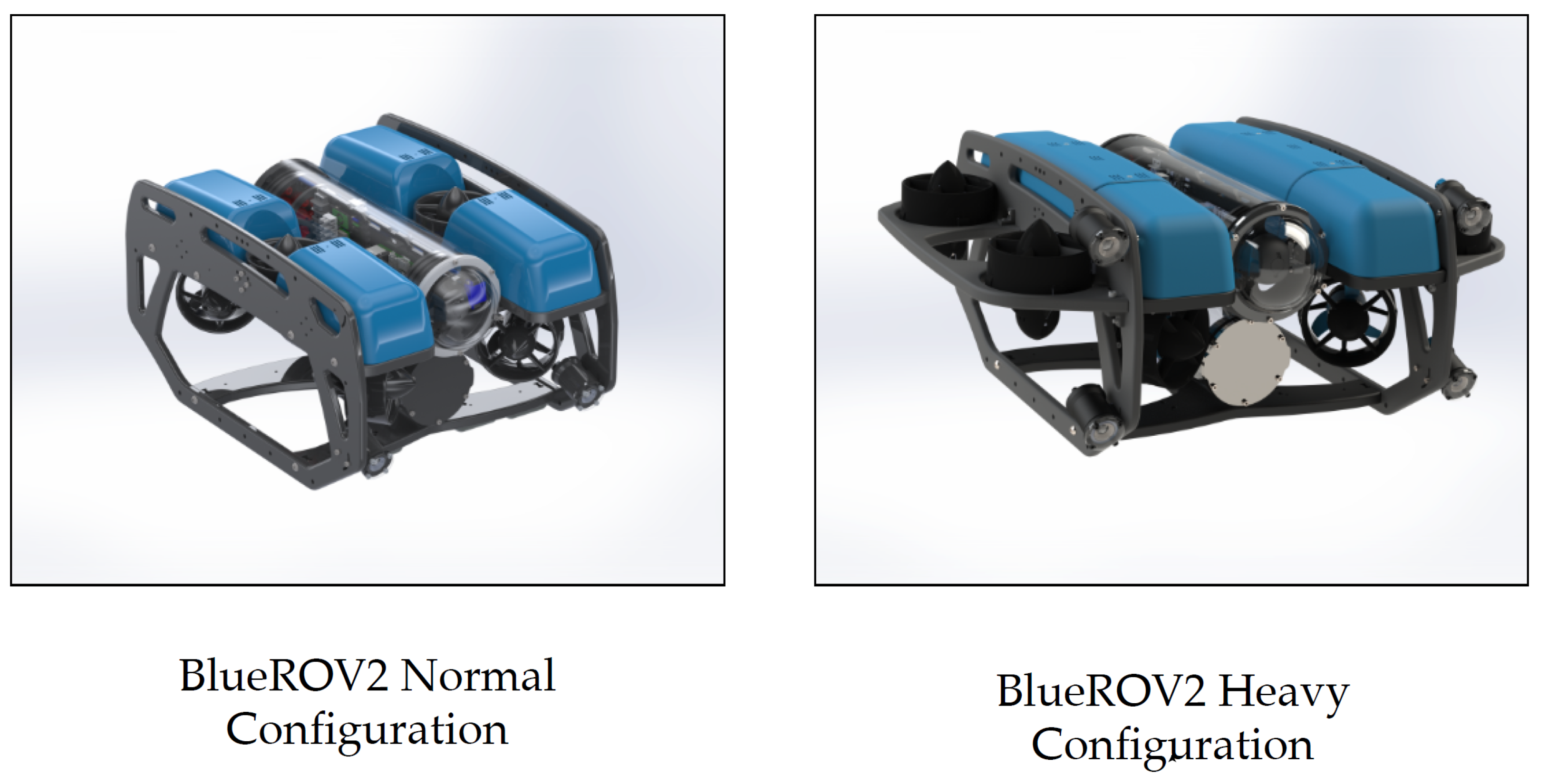
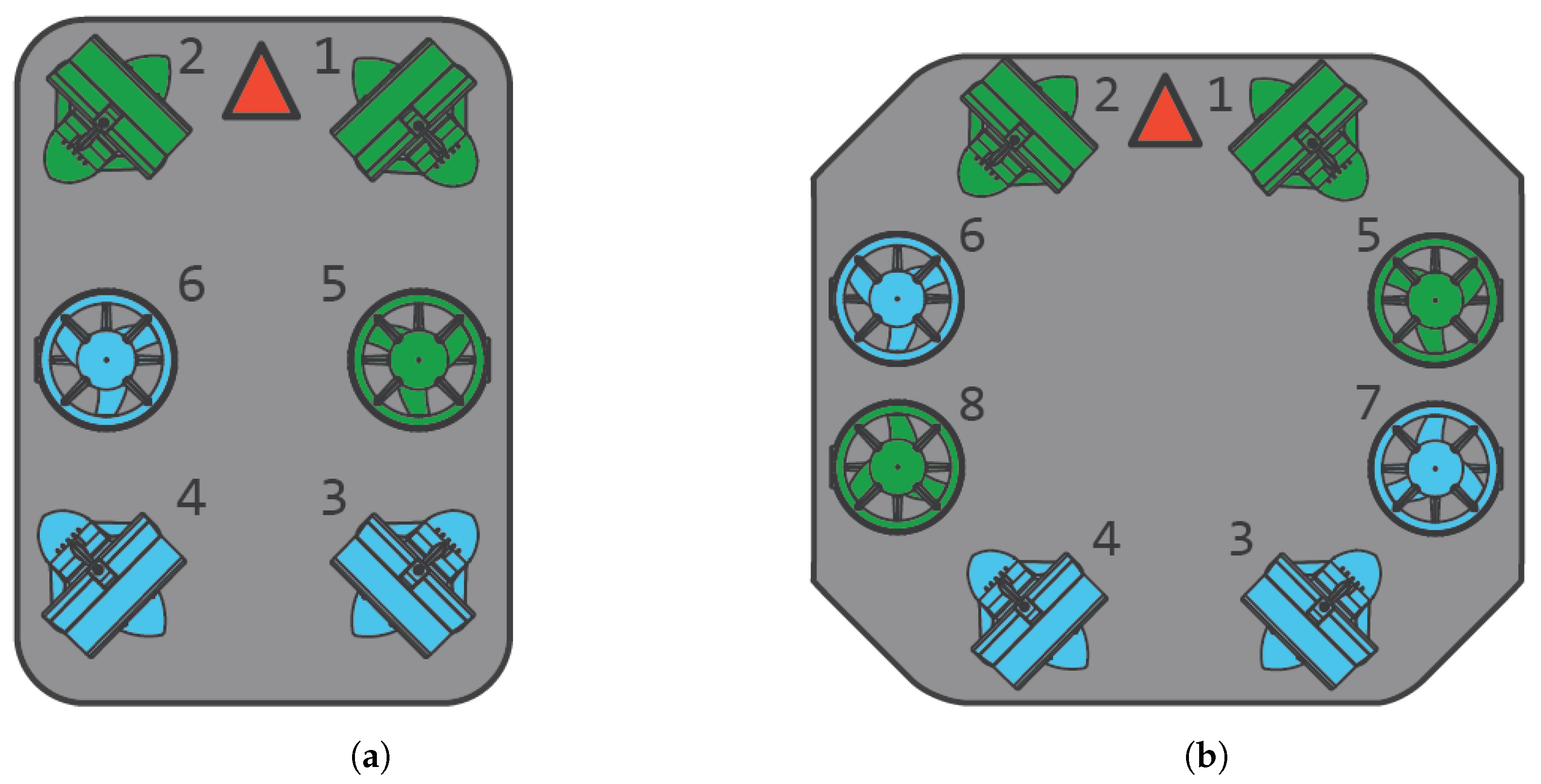
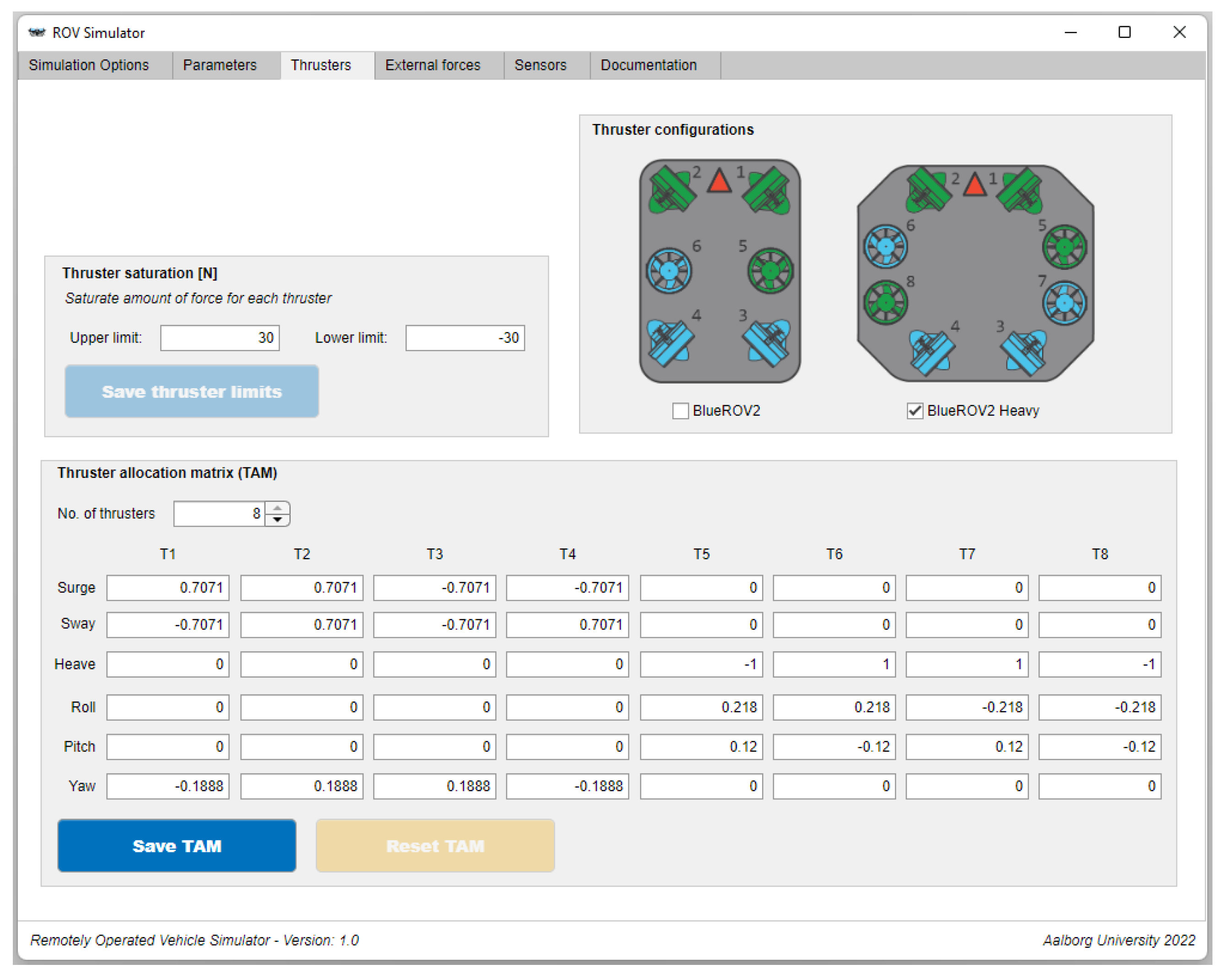
Blue Robotics Inc.’s heavy configuration kit is installed as additional equipment on the BlueROV2, which includes two additional T200 thrusters, such that the thrusters can be paired to move in all degrees of freedom. This modification is illustrated in Figure 2. The difference in thruster allocation between the normal and the heavy configuration is shown in Figure 3 and

Table 2. Difference between thruster combination to motion on normal and heavy configuration.

Motion	Normal BlueROV2	Heavy BlueROV2
Surge	T1, T2, T3 and T4	T1, T2, T3 and T4
Sway	T1, T2, T3 and T4	T1, T2, T3 and T4
Heave	T5 and T6	T5, T6, T7 and T8
Roll	T5 and T6	T5, T6, T7 and T8
Pitch	Uncontrollable	T5, T6, T7 and T8
Yaw	T1, T2, T3 and T4	T1, T2, T3 and T4

, the most noticeable difference is that the heavy configuration is controllable in pitch. Tools can be installed for specific operations, such as a gripper (purchased together with the BlueROV2), a water jet [3], etc.

3. Mathematical Modeling

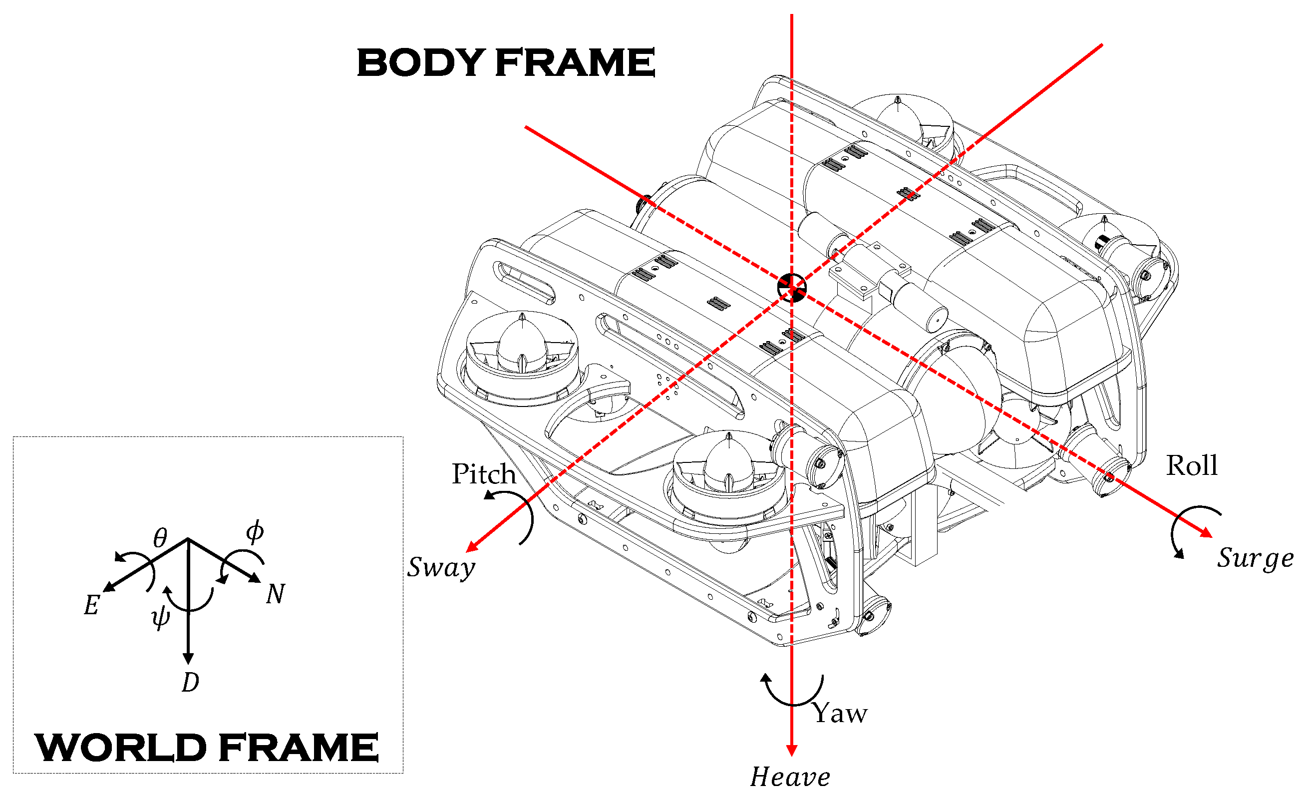
In the following, we will distinguish between the body or b-frame and world or n-frame as illustrated in Figure 4, where the respective degrees of freedom are visualized in each frame.

In this section, we recall the standard mathematical model of an underwater vehicle, to which the BlueROV2 applies. This model is based on the following few assumptions:

Assumption 1.

The vehicle is assumed to be rigid, and 6 degrees of freedom are considered.

Assumption 2.

The ROV is assumed symmetric around the front-back, port-starboard and the top-bottom axes.

Assumption 3.

The body axes coincide with the principles axes of inertia.

Assumption 4.

The origin of the b-frame is located at the center of mass of the vehicle.

Remark 1.

The Assumptions 1–4 are common when modeling underwater vehicles [26].

Assumption 5.

The ocean current is modeled as a constant irrotational flow in the n-frame. The current is projected on the ROV as a change in velocity. Waves are neglected.

Remark 2.

The Assumption 5 is a simplified model of the current, as ocean currents are mainly caused by tidal movements and can be dependent on both the local climate and the geographic characteristics [27]. Furthermore, the current velocity varies both with space and time. However, from a control perspective where the current acts as a disturbance to the system, the time dependency can be neglected due to the relatively slowly varying current compared to the dynamics of the controlled system [26].

In the following, we will use the well-known compact $\mathbf{\eta }-\mathbf{\nu }$ Fossen notation (first proposed in [28]), itself gathering in a vectorial form elements of the SNAME nomenclature (see [29,30], and a list of the variables and parameters used hereafter summarized in

Table 3. Definitions of variables.

Notation	Description
$\mathit{C},{\mathit{C}}_{RB},{\mathit{C}}_A$	System/rigid-body/added-mass Coriolis
	-centripetal matrix
$\mathit{D}$	Vector of damping forces
$F,M$	External forces and moments acting on the
	vehicle in the b-frame
$\mathit{g}$	Vector of restoring forces
$\mathit{J}$	Coordinate transformation matrix
$\mathit{M},{\mathit{M}}_{RB},{\mathit{M}}_A$	System/rigid-body/added-mass inertia matrix
m	Total mass of the vehicle
$p,q,r$	Angular velocities in the b-frame
$u,v,w$	Linear velocities in the b-frame
$\mathit{v}$	Linear velocity vector in the b-frame
$X,Y,K,N_{\dot{u}-\dot{r}}$	Added mass coefficients in the b-frame
$x,y,z$	Translation in the n-frame
$x_b,y_b,z_b$	Body-fixed reference frame (b-frame)
$\mathbf{\eta }$	Vector of position and orientation in the n-frame
$\mathbf{\nu }$	Velocity vector in the b-frame
$\rho$	Water density
$\mathbf{\tau }$	Vector of control inputs
$\varphi ,\theta ,\psi$	Euler’s angles in the n-frame
$\mathbf{\omega }$	Angular velocity vector in the b-frame

). It is given by

$$\dot{\mathbf{\eta }}=\mathit{J}\left(\mathit{\eta }\right)\mathit{\nu }$$

(1)

$$\begin{array}{cc}\hfill \mathit{M}\dot{\mathit{\nu }}+\mathit{C}\left(\mathit{\nu }\right)\mathit{\nu }+\mathit{D}\left(\mathit{\nu }\right)\mathit{\nu }+\mathit{g}\left(\mathit{\eta }\right)& =\mathit{\tau }+{\mathit{\tau }}_{tet}\hfill \end{array}$$

(2)

where $\mathit{\nu }={[u,v,w,p,q,r]}^T$ is the vector of body-fixed velocities (surge, sway, heave, roll, pitch and yaw) and $\mathbf{\eta }={[x,y,z,\varphi ,\theta ,\psi ]}^T$ is the vector combining the positions and Euler angles with respect to the n-frame. The vector $\mathbf{\tau }={[X,Y,Z,K,M,N]}^T$ contains the forces and moments applied to the vehicle.

Equation (1) represents the kinematic equations of motion, where

$$\mathit{J}\left(\mathit{\eta }\right)=\left[\begin{array}{cc}{\mathit{J}}_1\left(\mathit{\eta }\right)& {\mathit{0}}_{3\times 3}\\ {\mathit{0}}_{3\times 3}& {\mathit{J}}_2\left(\mathit{\eta }\right)\end{array}\right],$$

(3)

and

$${\mathit{J}}_1\left(\mathit{\eta }\right)=\left[\begin{array}{ccc}cos\psi cos\theta & -sin\psi cos\varphi +cos\psi sin\theta sin\varphi & sin\psi sin\varphi +cos\psi cos\varphi sin\theta \\ sin\psi cos\theta & cos\psi cos\varphi +sin\varphi sin\theta sin\psi & -cos\psi sin\varphi +sin\theta sin\psi cos\varphi \\ -sin\theta & cos\theta sin\varphi & cos\theta cos\varphi \end{array}\right]$$

(4)

$${\mathit{J}}_2\left(\mathit{\eta }\right)=\left[\begin{array}{ccc}1& sin\varphi tan\theta & cos\varphi tan\theta \\ 0& cos\varphi & -sin\varphi \\ 0& sin\varphi /cos\theta & cos\varphi /cos\theta \end{array}\right],$$

(5)

where let us recall that ${\mathit{J}}_2\left(\mathit{\eta }\right)$ is not defined when $\theta =\{-\pi ,\pi \}\left[2\pi \right]$.

The constant, symmetric and strictly positive definite inertia matrix $\mathit{M}={\mathit{M}}_{RB}+{\mathit{M}}_A$ combines the rigid-body inertia matrix ${\mathit{M}}_{RB}$ given by

$${\mathit{M}}_{RB}=\left[\begin{array}{cc}m{\mathit{I}}_{3\times 3}& {\mathit{0}}_{3\times 3}\\ {\mathit{0}}_{3\times 3}& {\mathit{I}}_c\end{array}\right]$$

(6)

with ${\mathit{I}}_c=diag\{I_x,I_y,I_z\}$, and the added-mass and inertia matrix, which we assume to be diagonal containing the added-mass coefficients, so that we have

$${\mathit{M}}_A=-diag\{X_{\dot{u}},Y_{\dot{v}},Z_{\dot{w}},K_{\dot{p}},M_{\dot{q}},N_{\dot{r}}\}.$$

(7)

Skew-symmetric Coriolis matrix $\mathit{C}\left(\mathit{\nu }\right)={\mathit{C}}_{RB}\left(\mathit{\nu }\right)+{\mathit{C}}_A\left(\mathit{\nu }\right)$ also combines rigid-body and hydrodynamics effects, with

$${\mathit{C}}_{RB}=\left[\begin{array}{cccccc}0& 0& 0& 0& mw& -mv\\ 0& 0& 0& -mw& 0& mu\\ 0& 0& 0& mv& -mu& 0\\ 0& mw& -mv& 0& -I_{z}r& -I_{y}q\\ -mw& 0& mu& I_{z}r& 0& I_{x}p\\ mv& -mu& 0& I_{y}q& -I_{x}p& 0\end{array}\right]$$

(8)

and

$${\mathit{C}}_A=\left[\begin{array}{cccccc}0& 0& 0& 0& -Z_{\dot{w}}w& Y_{\dot{v}}v\\ 0& 0& 0& Z_{\dot{w}}w& 0& -X_{\dot{u}}u\\ 0& 0& 0& -Y_{\dot{v}}v& X_{\dot{u}}u& 0\\ 0& -Z_{\dot{w}}w& Y_{\dot{v}}v& 0& -N_{\dot{r}}r& M_{\dot{q}}q\\ Z_{\dot{w}}w& 0& -X_{\dot{u}}u& N_{\dot{r}}r& 0& -K_{\dot{p}}p\\ -Y_{\dot{v}}v& X_{\dot{u}}u& 0& -M_{\dot{q}}q& K_{\dot{p}}p& 0\end{array}\right]$$

(9)

At low-speed, the hydrodynamic damping matrix $\mathit{D}\left(\mathit{\nu }\right)=\mathit{D}+{\mathit{D}}_n\left(\mathit{\nu }\right)$ is considered without coupling, so that we have the diagonal matrices containing the linear and nonlinear damping coefficients

$$\mathit{D}=-diag(X_u,Y_v,Z_w,K_p,M_q,N_r)$$

(10)

and

$${\mathit{D}}_n\left(\nu \right)=-diag{X}_{u\left|u\right|}\left|u\right|,Y_{v\left|v\right|}\left|v\right|,Z_{w\left|w\right|}\left|w\right|,K_{p\left|p\right|}\left|p\right|,M_{q\left|q\right|}\left|q\right|,N_{r\left|r\right|}\left|r\right|),$$

(11)

the latter diagonal matrix representing quadratic damping.

Taking into account Assumption 4, the vector of restoring forces (gravitational and buoyancy forces) $\mathit{g}\left(\mathit{\eta }\right)$ is expressed as

$$\mathit{g}\left(\mathit{\eta }\right)=\left[\begin{array}{c}(W-B)sin\theta \\ -(W-B)cos\theta sin\varphi \\ -(W-B)cos\theta cos\varphi \\ y_{b}Bcos\theta cos\varphi -z_{b}Bcos\theta sin\varphi \\ -z_{b}Bsin\theta -x_{b}Bcos\theta cos\varphi \\ x_{b}Bcos\theta sin\varphi +y_{b}Bsin\theta \end{array}\right].$$

(12)

where $W=mg$ and $B=\rho g\nabla$ are the gravity and buoyancy forces, respectively ($\rho$ the water density and ∇ the volume of fluid displaced by the vehicle), and $(x_b,y_b,z_b)$ are the coordinates of the center of buoyancy expressed in the b-frame.

An ROV like the BlueROV2 is typically actuated by a number r of fixed thrusters. In order to link the vector $\tau$ to the voltages $V_i$ applied to each thruster i ($i\in \{1,\cdots ,r\}$), we use the expression

$$\tau =\mathit{T}\mathit{K}\left(s\right)\mathit{F}\left(\mathit{V}\right)$$

(13)

with $\mathit{V}={[V_1,\cdots ,V_r]}^T$ denoting thruster voltages in column vector $\mathit{F}\left(\mathit{V}\right)$. Matrix $\mathit{T}\in {\mathbb{R}}^{6\times r}$ is the so-called thrust configuration matrix (see [24]):

$$\mathit{T}=[{\mathit{t}}_1,\cdots ,{\mathit{t}}_r]$$

(14)

thereby, we obtain the thruster mixing matrix, where each column vector ${\mathit{t}}_i$ links the force $F_i$ created by each thruster to vector $\tau$:

$${\mathit{t}}_i=\left[\begin{array}{c}{\epsilon }_i\\ {\mathit{r}}_i\times {\epsilon }_i\end{array}\right]$$

(15)

where ${\epsilon }_i$ is a unit vector representing the orientation of thruster i and ${\mathit{r}}_i$ is the distance between the point of application of the force $F_i$ and the center of the b-frame.

The diagonal matrix $\mathit{K}\left(s\right)$ contains unity DC-gain transfer functions accounting for the dynamic relation between $V_i$ and the force $F_i$, i.e., we have

$$\mathit{K}\left(s\right)=diag(K_1\left(s\right),\cdots ,K_r\left(s\right)).$$

(16)

4. Parameter Identification and Model Validation

This section covers the identification procedure and validation of model parameters listed in

Table A1. Evaluation of parameters.

Notation	Value	Unit	Origin
g	$9.82$	$\frac{\mathrm{m}}{{\mathrm{s}}^2}$	-
$\rho$	1000	$\frac{\mathrm{kg}}{{\mathrm{m}}^3}$	-
m	$13.5$	kg	Experimental
∇	$0.0134$	m${}^3$	Experimental
$I_x$	$0.26$	$\mathrm{kg}·{\mathrm{m}}^2$	CAD
$I_y$	$0.23$	$\mathrm{kg}·{\mathrm{m}}^2$	CAD
$I_z$	$0.37$	$\mathrm{kg}·{\mathrm{m}}^2$	CAD
$(x_g,y_g,z_g)$	$(0,0,0)$	m	Defined
$(x_b,y_b,z_b)$	$(0,0,-0.01)$	m	CAD
${\mathit{r}}_{\mathit{i}}$ for $i=\{1,2,3,4\}$	${\mathit{J}}_3\left({\alpha }_i\right)$${\left[\begin{array}{ccc}0.156& 0.111& 0.085\end{array}\right]}^T$ for ${\alpha }_i=\{0,5.05,1.91,\pi \}$
${\mathbf{\epsilon }}_i$ for $i=\{1,2,3,4\}$	${\mathit{J}}_3\left({\beta }_i\right)$${\left[\begin{array}{ccc}1/\sqrt{2}& -1/\sqrt{2}& 0\end{array}\right]}^T$ for ${\beta }_i=\{0,\frac{\pi }{2},\frac{3\pi }{4},\pi \}$	m	CAD
${\mathit{r}}_{\mathit{i}}$ for $i=\{5,6,7,8\}$	${\mathit{J}}_3\left({\gamma }_i\right)$${\left[\begin{array}{ccc}0.120& 0.218& 0\end{array}\right]}^T$ for ${\gamma }_i=\{0,4.15,1.01,\pi \}$
${\mathbf{\epsilon }}_i$ for $i=\{5,6,7,8\}$	${\left[\begin{array}{ccc}0& 0& -1\end{array}\right]}^T$
$X_u$	13.7	$\frac{\mathrm{Ns}}{\mathrm{m}}$
$X_{u\left|u\right|}$	141.0	$\frac{{\mathrm{Ns}}^2}{{\mathrm{m}}^2}$
$Y_v$	0	$\frac{\mathrm{Ns}}{m}$
$Y_{v\left|v\right|}$	217.0	$\frac{{\mathrm{Ns}}^2}{{\mathrm{m}}^2}$
$Z_w$	33.0	$\frac{\mathrm{Ns}}{\mathrm{m}}$
$Z_{w\left|w\right|}$	190.0	$\frac{{\mathrm{Ns}}^2}{{\mathrm{m}}^2}$	Experimental
$K_p$	0	$\frac{\mathrm{Ns}}{\mathrm{m}}$
$K_{p\left|p\right|}$	1.19	$\frac{{\mathrm{Ns}}^2}{{\mathrm{m}}^2}$
$M_q$	0.8	Ns
$M_{q\left|q\right|}$	0.47	Ns${}^2$
$N_r$	0	Ns
$N_{r\left|r\right|}$	1.5	Ns${}^2$
$X_{\dot{u}}$	$6.36$	kg
$Y_{\dot{v}}$	$7.12$	kg
$Z_{\dot{w}}$	$18.68$	kg	[33]
$K_{\dot{p}}$	$0.189$	$\mathrm{kg}{\mathrm{m}}^2$
$M_{\dot{q}}$	$0.135$	$\mathrm{kg}{\mathrm{m}}^2$
$N_{\dot{r}}$	$0.222$	$\mathrm{kg}{\mathrm{m}}^2$
$m_{tet}$	$0.043$	kgm${}^{-1}$	Experimental
$d_{tet}$	$0.0075$	m	Experimental
$C{n}_{tet}$	$1.2$	–	[41]
$C{t}_{tet}$	$0.01$	–	[41]
$C_{tet}$	100	Nsm${}^{-1}$	[41]
$E_{tet}$	$6.437\times {10}^{10}$	N/m${}^2$	[41]

. Table A1 specifies whether the parameter is determined from experiments, from a CAD-model, or obtained from other sources.

4.1. Thruster Model

The BlueROV2 in heavy configuration is built with eight T200 thrusters. The numbering and loci follow the definition of the manufacturer [31]. The thruster orientation, ${\epsilon }_{\mathit{i}}$, location, ${\mathit{r}}_{\mathit{i}}$, is given in Table A1. The thrusters are located in a circular pattern and the rotation matrix used is denoted

$${\mathit{J}}_3\left(\alpha \right)=\left[\begin{array}{ccc}cos\alpha & -sin\alpha & 0\\ sin\alpha & cos\alpha & 0\\ 0& 0& 1\end{array}\right]$$

(17)

A nonlinear regression to normalized input voltages and measured force, $\mathit{F}\left(\mathit{V}\right)$, is obtained from experiments conducted in prior work [4]. The regression given for $V_i\in [-1,1]$ is

$$F_i\left(V_i\right)=-140.3V_i^9+389.9V_i^7-404.1V_i^5+176.0V_i^3+8.9V_i$$

(18)

The thruster dynamics is described by the diagonal transfer function matrix $\mathit{K}\left(s\right)=diag(K_1\left(s\right),\cdots ,K_r\left(s\right))$. The diagonal elements are equal and obtained from system identification on experimental data published by MathWorks [32]. The following third order transfer function with unity DC-gain was identified

$$K_i\left(s\right)=\frac{6136s+108700}{s^3+89s^2+9258s+108700}$$

(19)

The maximum velocities and forces of each direction of motion are shown in

Table 4. Maximum velocities and forces in b-frame.

Movement in b-Frame	Maximum Velocity	Maximum Thrust Force
${\dot{x}}_{max}$	$0.72$ ms${}^{-1}$	85 N
${\dot{y}}_{max}$	$0.63$ ms${}^{-1}$	85 N
${\dot{z}}_{max}$	$0.71$ ms${}^{-1}$	120 N
$p_{max}$	$5.2$ ms${}^{-1}$	26 Mm
$q_{max}$	$4.9$ ms${}^{-1}$	14 Nm
$r_{max}$	$3.6$ ms${}^{-1}$	22 Nm

.

4.2. Hydrodynamic Damping

The hydrodynamic damping coefficients given in Equations (10) and (11) are determined in a comparative study of the model output and from a series of experiments conducted in a 1.15 m deep 6.1 m diameter pool. The experiments are designed such that the ROV is actuated individually and in open-loop in all 6-DOF, one at a time, at an interval of several input voltages. Each experiment is conducted twice, where the first instance is used for estimating coefficients and the latter is used for validation. Rather than actuating the thrusters individually, the thrusters are actuated using the standard ArduSUB software allowing for actuating along the 6-DOF directly. The individual thruster input is logged during the experiments and used as input to the model.

The ROV is actuated in each direction of motion from just above the deadzone of the thrusters at 20% input to 100% input, with a step-wise increase of 10%. As an example of one of these tests, Figure 5 compares the experimental data and the model output given 50% input in the surge direction. Position feedback is obtained by using a UAPS Short BaseLine (SBL) location system. The disturbance from tether forces is reduced by manually maneuvering the tether in the direction of the ROV, but it has not been possible to eliminate this disturbance entirely. As a consequence, a proportional feedback controller is used for regulating to a constant depth to ensure that the ROV does not hit the pool bottom or water surface during the surge and sway-direction experiments.

As seen in Figure 5, the thrusters are activated after 20 s. The quasi-static part of the motion is used for determining the velocity and consequently the difference between the simulation model and experimental measurements. Figure 6 shows the error for an interval of inputs from just above the deadzone of the thrusters to maximum input, from 20% to 100% input. The largest model discrepancy for both the surge and sway direction of motion is approximately 10%.

Hydrodynamic coefficients related to the heave motion are estimated and validated by performing an experiment where the ROV is submerged at the bottom of the pool and actuating thrusters in the negative heave direction. The heave motion is determined using the pressure sensor. Figure 6 shows that the heave motion model error for the thrust input of 20% is 15% and that the error reduces for larger inputs.

Rotational motion in pitch, roll, and yaw is validated using the integrated Inertial Measurement Unit (IMU) for angular velocity measurement. It is necessary to fully rotate the ROV during the rotational drag tests. This requires an input of more than 30%. Therefore, for the rotational motions, the input given is from 30% to 100% with a step-wise increase of 10%. The model discrepancy for pitch, roll, and yaw is seen in Figure 7. Roll motion error is seen to increase at higher inputs to approximately 10%. The largest discrepancy between the model and experiment for pitch and yaw rotation is 10% and 12%, respectively.

The error bars shown in Figure 6 and Figure 7 show the error between the corrected simulation model and the validation data. There is no clear pattern in the error to further optimize the second order polynomial model. If the hydrodynamic model should be further improved, this requires more precise measurements along with more tests to obtain knowledge about the tendency of the error. This has not been deemed necessary.

4.3. Added Mass

Added mass coefficients presented in Equation (7) are estimated from Eidsvik method [33], which builds upon the experimental work outlined by Det Norske Veritas (DNV) [34]. Eidsvik shows that the relative error of the empirical estimations in translational and rotational degrees of freedom are 10–20% and 30–100%, respectively. The method requires overall dimensions and projected areas of the ROV. The method also requires that the difference in overall dimensions is not larger than 10%. The BlueROV2 in heavy configuration violates this requirement as the width is 20% larger than the length, and the estimated added mass coefficients may be susceptible to further error than predicted by Eidsvik. This will lead to a difference between the model and the physical robot in the acceleration phase. The overall dimensions and projected areas are given in

Table 5. Overall dimensions and projected areas of the BlueROV2 heavy configuration.

Notation	Value	Unit
L × H × W	$0.46$ × $0.38$ × $0.58$	m
$A_u$	$0.0877$	m${}^2$
$A_v$	$0.1131$	m${}^2$
$A_w$	$0.2049$	m${}^2$

and are found using a CAD model of the ROV. L, H, and W, denote the length, height, and width. The notation for the projected areas is given such that the subscript shows the normal direction to the area in the b-frame. The resulting added mass coefficients are found in Table A1.

5. Ocean Current

The current effect is implemented as an additional velocity term that does not change in the water column. The velocity term in the equations of motions given in Equation (2) is thereby transformed to be in terms of relative velocity shown in Equation (20),

$$\left({\mathbf{M}}_{rb}\dot{\mathbf{v}}+{\mathbf{C}}_{rb}\left(\mathbf{v}\right)\mathbf{v}+\mathbf{g}\left(\mathbf{\eta }\right))\right)+\left({\mathbf{M}}_A{\dot{\mathbf{v}}}_r+{\mathbf{C}}_A\left({\mathbf{v}}_r\right){\mathbf{v}}_r+\mathbf{D}\left({\mathbf{v}}_r\right){\mathbf{v}}_r\right)=\mathbf{\tau }+{\mathbf{\tau }}_{\mathit{tet}}$$

(20)

where the relative velocity is given by ${\mathbf{v}}_r=\mathbf{v}-{\mathbf{v}}_c$. As it is assumed that the current is irrotational, the vector for the water particles velocity in b-frame ${\mathbf{v}}_c$ becomes

$${\mathbf{v}}_c=\mathbf{R}{\mathbf{\upsilon }}_c$$

(21)

where,

$${\upsilon }_c={\left({\dot{u}}_c,{\dot{j}}_c,{\dot{w}}_c,0,0,0\right)}^{\top }$$

(22)

where ${\dot{u}}_c,{\dot{j}}_c,{\dot{w}}_c$ is the n-frame water particle velocity in north, east and down direction, respectively. As the current is represented in n-frame, this velocity can be transformed into b-frame by the inverse rotation matrix such that it can be implemented in the model represented in b-frame.

From Equation (8), it is shown that ${\mathit{C}}_{rb}$ is parameterized independent of linear velocity, and it is assumed that the current is slowly varying, so that the velocity can be assumed to be constant. Therefore, Equation (20) can be reduced to

$$\mathbf{M}\dot{\mathbf{v}}+\mathbf{C}\left(\mathbf{v}\right)\mathbf{v}+\mathbf{D}\left({\mathbf{v}}_r\right){\mathbf{v}}_r+\mathbf{g}\left(\eta \right)=\tau +{\tau }_{\mathit{tet}}$$

(23)

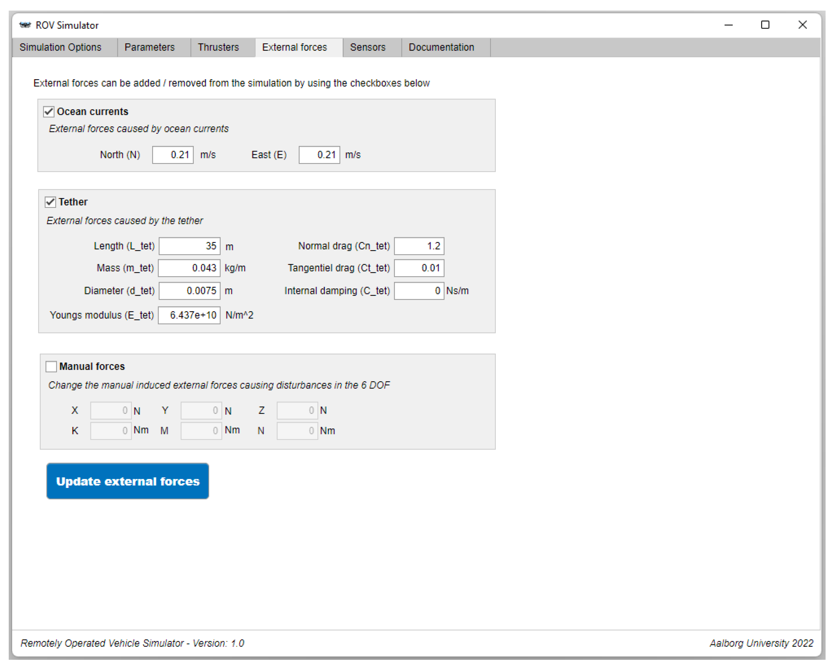
6. Tether Model

In most underwater applications, the tether is used for communication and power from the top-side, therefore it is a necessity. However, the tether also disturbs the ROV due to the forces generated by the drag and underwater currents [35]. The proposed simulator also includes the dynamics of the tether linking the BlueROV2 underwater vehicle to the top-site base. In order to model the tether, we use a lumped-mass approach, whereby the cable is idealized as a set of $n+1$ lumped masses connected together by n weightless cylinders [36,37].

Let ${\mathbf{p}}_i\in {\mathbb{R}}^3,i\in \{0,\cdots ,n\}$ represent the position of node/lumped mass i in the n-frame, and ${\mathbf{v}}_i:={\dot{\mathbf{p}}}_i$ the corresponding velocity vector. In this setting, ${\mathbf{p}}_0$ is directly linked to the above-mentioned base, whose position is possibly time-varying, i.e., ${\mathbf{p}}_0={\mathbf{p}}_b\left(t\right)$, while ${\mathbf{p}}_n$ is attached to the ROV. Hence, regarding the tether dynamics, let us group the remaining ${\mathbf{p}}_i$s and ${\mathbf{v}}_i$s into the vectors

$${\mathbf{p}}_t={[{\mathbf{p}}_1^T,{\mathbf{p}}_2^T,\cdots ,{\mathbf{p}}_{n-1}^T]}^T$$

(24)

and

$${\mathbf{v}}_t={[{\mathbf{v}}_1^T,{\mathbf{v}}_2^T,\cdots ,{\mathbf{v}}_{n-1}^T]}^T.$$

(25)

The dynamics associated with the tether position and velocity vectors ${\mathbf{p}}_t$ and ${\mathbf{v}}_t$ are summarized by the mass-spring-damper-like expression

$${\mathbf{M}}_t{\dot{\mathbf{v}}}_t+{\mathbf{D}}_t{\mathbf{v}}_t+{\mathbf{k}}_t=0$$

(26)

where ${\mathbf{M}}_t$ is a diagonal matrix of $n-1$ elements

$${\mathbf{M}}_{t,i}=\frac{1}{2}\left({\mathbf{M}}_{i-1}+{\mathbf{M}}_i+{\mathbf{M}}_{a,i-1}+{\mathbf{M}}_{a,i}\right)$$

(27)

where $M_i\in {\mathbb{R}}^{3\times 3}$ is the mass matrix of node i and $M_{a,i}\in {\mathbb{R}}^{3\times 3}$ is the added mass matrix of the corresponding cylinder. Similarly, the damping terms of diagonal matrix ${\mathbf{D}}_t$ are given by

$${\mathbf{D}}_{t,i}={\mathbf{P}}_{i-1}-{\mathbf{P}}_i+{\mathbf{F}}_i$$

(28)

where ${\mathbf{P}}_i$, the internal damping of the tether, is expressed as

$${\mathbf{P}}_i=C_t\left[{({\mathbf{v}}_i-{\mathbf{v}}_{i-1})}^T\frac{{\mathbf{r}}_i}{|{\mathbf{r}}_i|}\right]\frac{{\mathbf{r}}_i}{|{\mathbf{r}}_i|}$$

(29)

where $C_t$ is a damping constant, and ${\mathbf{r}}_i:={\mathbf{p}}_{i+1}-{\mathbf{p}}_i$ is the vector between two consecutive nodes.

The tether being assumed to be neutrally buoyant, the external force ${\mathbf{F}}_i$ acting on element i of the tether represents only hydrodynamic drag. Then, force ${\mathbf{F}}_i$ is the sum of its normal and tangential components

$${\mathbf{F}}_i={\mathbf{F}}_{\perp ,i}+{\mathbf{F}}_{\Vert ,i}$$

(30)

where

$${\mathbf{F}}_{\perp ,i}=\frac{1}{2}\rho d_t{C}_{\perp }{\mathbf{v}}_{\perp ,i}|{\mathbf{v}}_{\perp ,i}||{\mathbf{r}}_i|$$

(31)

and

$${\mathbf{F}}_{\Vert ,i}=\frac{1}{2}\rho d_t{C}_{\Vert }{\mathbf{v}}_{\Vert ,i}|{\mathbf{v}}_{\Vert ,i}||{\mathbf{r}}_i|,$$

(32)

where $d_t$ is the diameter of the tether, ${\mathbf{v}}_{\perp ,i}$ and ${\mathbf{v}}_{\Vert ,i}$ are the normal and tangential components of the flow velocity of the i-th cylinder, while $C_{\perp }$ and $C_{\Vert }$ are their respective drag coefficients. The normal and tangential velocity components are obtained through the expressions

$${\mathbf{v}}_{\perp ,i}=\frac{\left[{({\upsilon }_c-{\mathbf{v}}_i)}^T{\mathbf{r}}_i\right]{\mathbf{r}}_i}{|{\mathbf{r}}_i{|}^2}$$

(33)

with ${\upsilon }_c$ representing the water current velocity, expressed in the n-frame and

$${\mathbf{v}}_{\Vert ,i}={\mathbf{\upsilon }}_c-{\mathbf{v}}_i-{\mathbf{v}}_{\perp ,i}.$$

(34)

The term ${\mathbf{k}}_t$ in (26) is given by

$${\mathbf{k}}_{t,i}={\mathbf{T}}_i$$

(35)

where the axial tension ${\mathbf{T}}_i$ of the i-th node is given by

$${\mathbf{T}}_i=E_t\left(\frac{A_{t,i}}{l_{0,i}}\right){\mathbf{r}}_i\left(1-\frac{l_{0,i}}{|{\mathbf{r}}_i|}\right),$$

(36)

The force acting on the ROV ${\tau }_{\mathit{tet}}$ is the end node of the axial tension.

Tether ROV Interaction

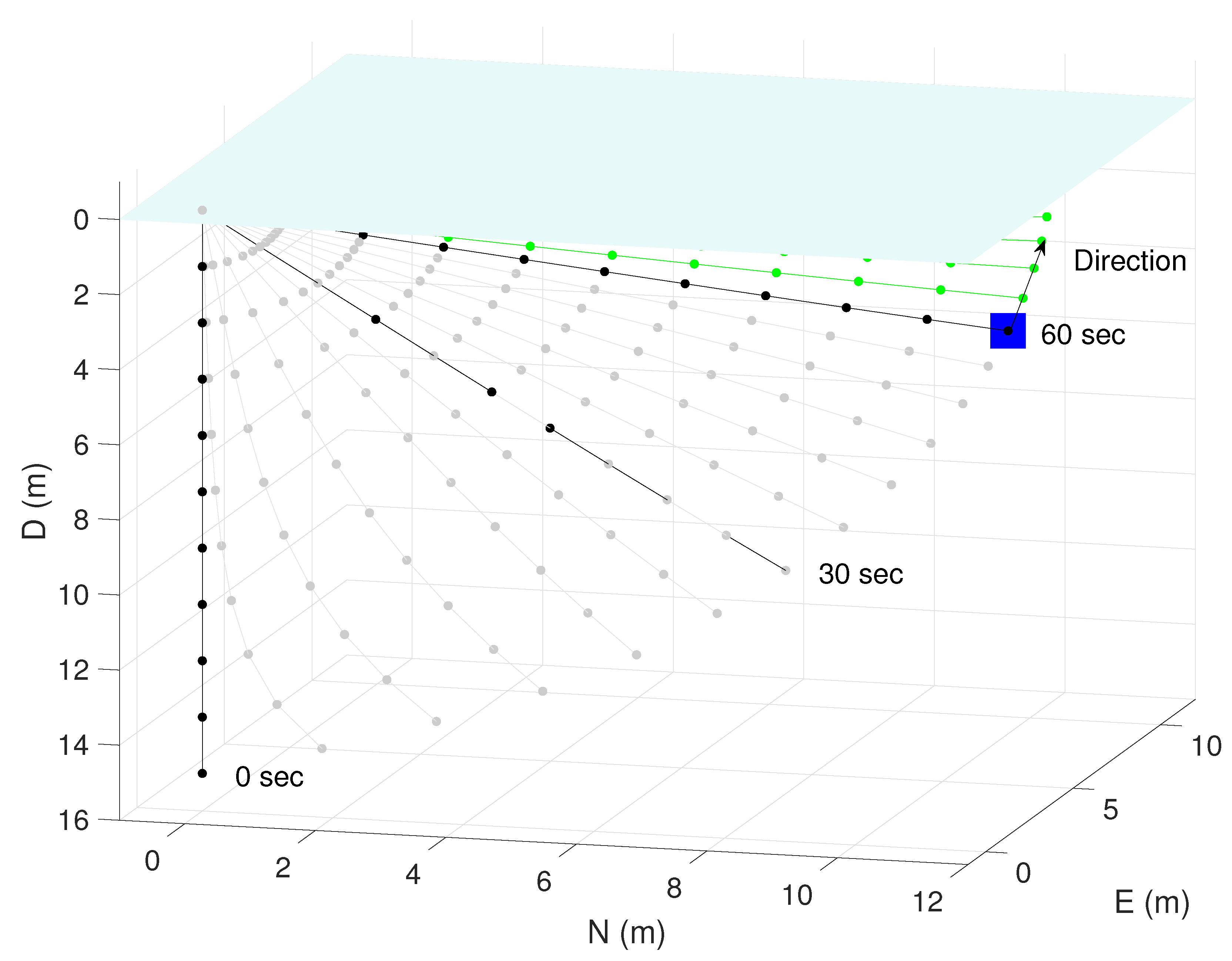
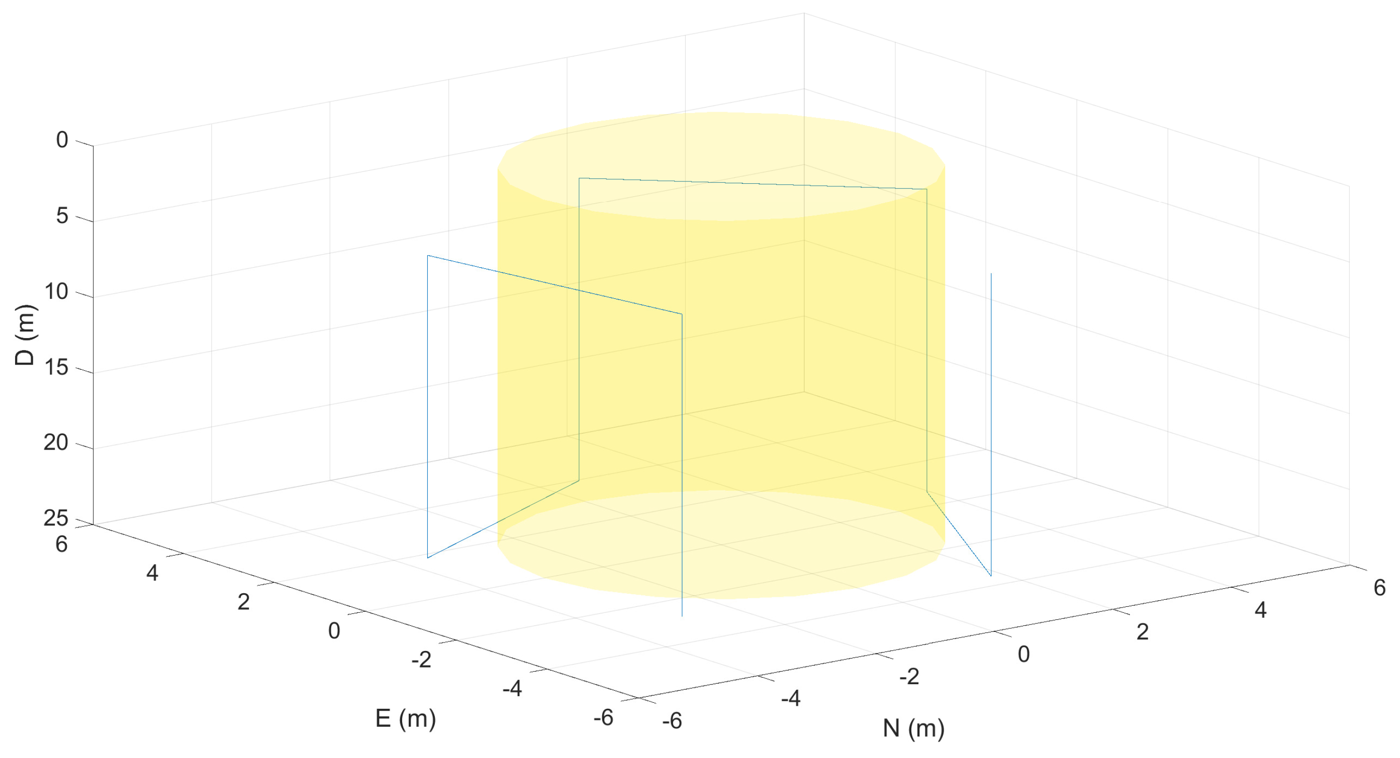
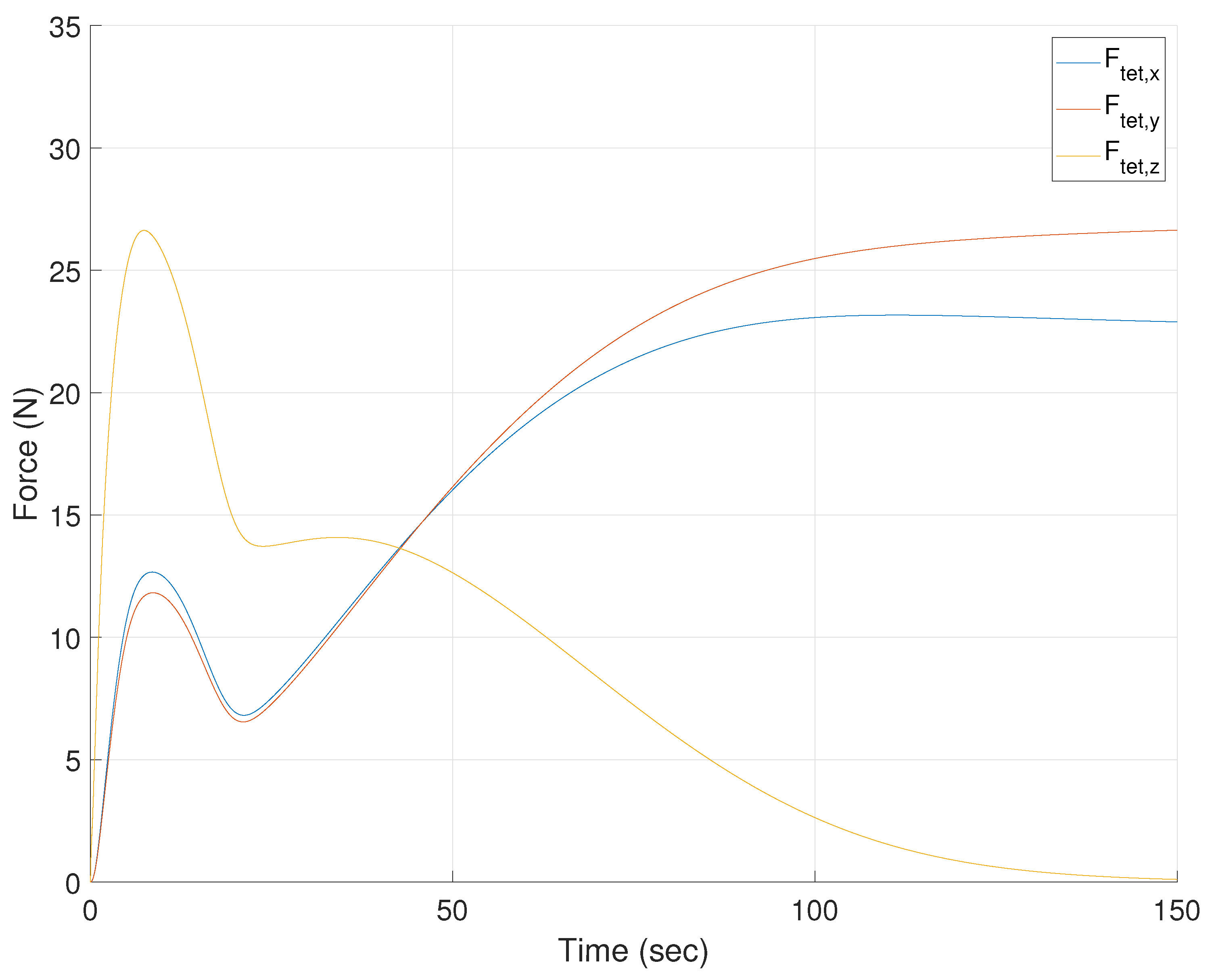
In the following, the ROV and tether interaction is demonstrated by letting the tethered ROV be free floating with a current velocity of $[0.3536,0.3536,0]$ in the n-frame and initialized at $[0,0,15]$. The tether is 15 m in length and with the tether parameters from Table A1. In Figure 8, a 3D plot of the ROV and tether is shown. This shows that the tether is initially lagging behind the ROV, but straightens out after 30 s. After 100 s, the ROV is approximately at the surface, and after 150 s, the force in x,y,z is constant, which is shown in Figure 9. 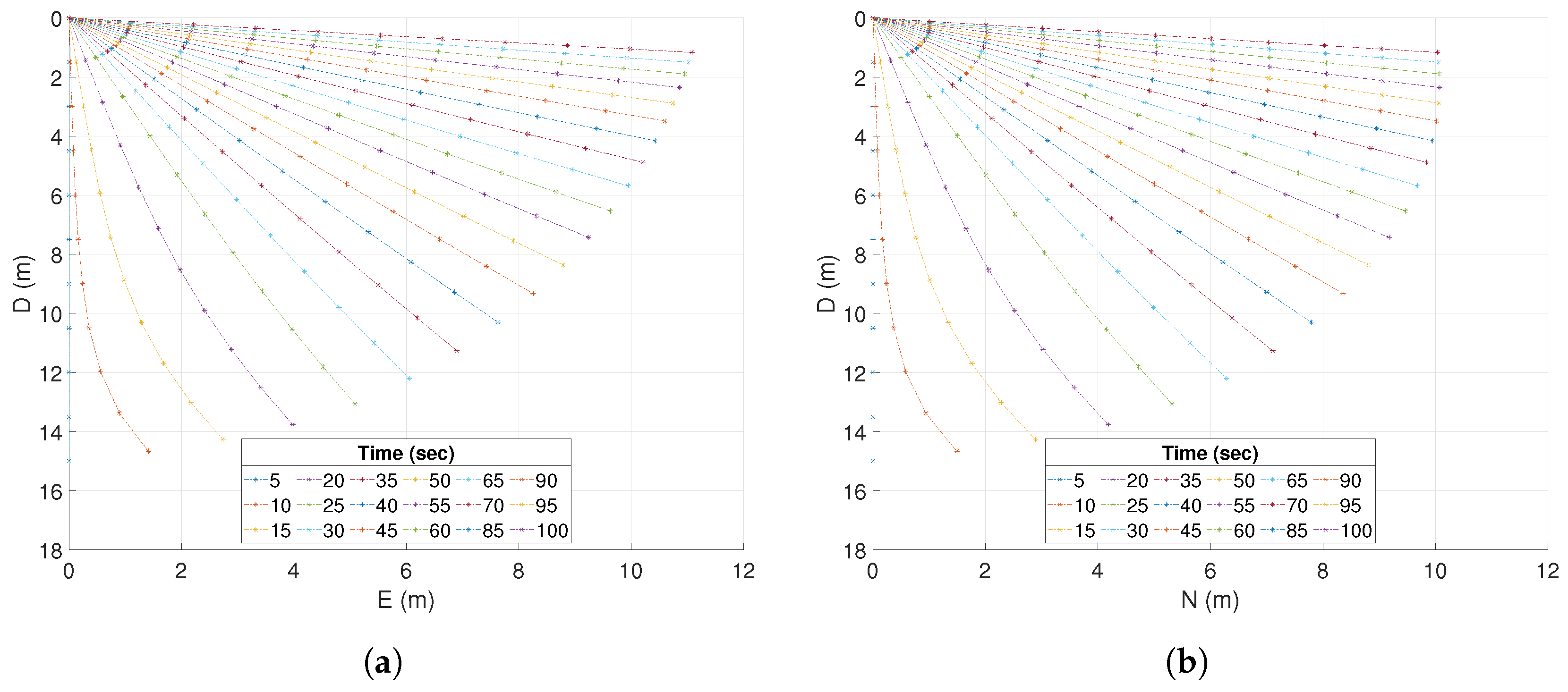When comparing the forces from Figure 9 to the maximum thrust force of the ROV seen in Table 4, it is clear that the tether has a large effect on the ROV. The movement in the Down-North and Down-East directions are shown in Figure 10. The range from 100–150 s is left out due to the change in position being minor. From Figure 10, it can be seen that the ROV moves further East compared to North, which is due to the drag force being larger.

A video of the free floating ROV and tether with a constant current velocity of $[0.3536,0.3536,0]$ in the n-frame can be found in the attached video named “Tether-ROV interaction” or at Github in Supplementary Materials.

7. Control Algorithms for Benchmarking

7.1. Sliding Mode Control

Sliding mode control (SMC) is a popular choice for control of underwater vehicles due to its ability to deal with nonlinear systems subject to uncertainties and bounded disturbances [38]. Moreover, it requires relatively low computer power to compute. The objective, for the sliding-mode controllers implemented on the BlueROV2 (one for each DOF), is to follow a pre-defined reference path given as

$${\mathit{\eta }}_r={[x_r,y_r,z_r,{\varphi }_r,{\theta }_r,{\psi }_r]}^T,$$

(37)

where we assume that the time-derivatives of ${\mathit{\eta }}_r$ exist and are bounded.

In the following, we design 6 sliding-mode controllers, one for each DOF, where ${\eta }_i$ is the i-th component of earth-fixed vector $\mathit{\eta }$. Then, we rewrite in component-form the system described by Equations (1) and (2) so that we have, for each component ${\eta }_i$,

$${\ddot{\eta }}_i=f_i({\eta }_i,{\dot{\eta }}_i,t)+{\overline{\tau }}_i,$$

(38)

where $f_i({\eta }_i,{\dot{\eta }}_i,t)$ is an unknown but bounded time-varying nonlinear function, with the explicit time dependence representing the coupling between the different DOFs. Control input ${\overline{\tau }}_i$ is the i-th component of vector $\overline{\mathit{\tau }}$, which is in turn given by $\overline{\mathit{\tau }}={\left[{\mathbf{J}}^{-T}\left(\mathit{\eta }\right)\mathbf{M}{\mathbf{J}}^{-1}\left(\mathit{\eta }\right)\right]}^{-1}{\mathbf{J}}^{-T}\left(\mathit{\eta }\right)\tau$. Defining now the tracking error of each of the 6 DOF as $e_i:={\eta }_i-{\eta }_{r,i}$ (with ${\eta }_{r,i}$ being the i-th component of vector ${\mathit{\eta }}_r$ in Equation (37)), the tracking error dynamics for each DOF is given by

$${\ddot{e}}_i=f_i({\eta }_i,{\dot{\eta }}_i,t)-{\ddot{\eta }}_{r,i}+{\overline{\tau }}_i.$$

(39)

From there, define first, for each DOF, the sliding variable

$${\sigma }_i:={\dot{e}}_i+c_{0,i}{e}_i,$$

(40)

where $c_{0,i}$ is a strictly positive constant.

Computing the time-derivative of ${\sigma }_i$ and using expression from Equation (39), we obtain

$${\dot{\sigma }}_i={\ddot{e}}_i+c_{0,i}{\dot{e}}_i=f_i({\eta }_i,{\dot{\eta }}_i,t)-{\ddot{\eta }}_{r,i}+{\overline{\tau }}_i+c_{0,i}{\dot{e}}_i.$$

(41)

Choose then the following sliding-mode control law:

$${\overline{\tau }}_i={\overline{\tau }}_{i,nom}+{\overline{\tau }}_{i,dis},$$

(42)

where the role of the so-called nominal control law ${\overline{\tau }}_{i,nom}$ is to cancel the known terms in Equation (41) and is given by

$${\overline{\tau }}_{i,nom}={\ddot{\eta }}_{r,i}-c_{0,i}{\dot{e}}_i,$$

(43)

so that Equation (41) is transformed into

$${\dot{\sigma }}_i={\sigma }_{i,dis}+f_i({\eta }_i,{\dot{\eta }}_i,t).$$

(44)

Finally, given the bound on unknown dynamics $f_i$,

$$|f_i({\eta }_i,{\dot{\eta }}_i,t)|\le {\overline{f}}_i,$$

(45)

where ${\overline{f}}_i$ is a strictly positive constant, the discontinuous control law ${\overline{\tau }}_{i,dis}$ reads

$${\overline{\tau }}_{i,dis}=-k_{i}sgn\left({\sigma }_i\right),$$

(46)

where $k_i$ is a strictly positive tuning gain, and where $sgn\left({\sigma }_i\right)$ is the signum function. Using standard Lyapunov analysis, the sliding-mode controller in Equations (40), (42), (43) and (46) can be proven to make the sliding variable ${\sigma }_i$ converge to the so-called sliding surface ${\sigma }_i=0$ in finite time as long as tuning gain $k_i$ is chosen such that $k_i>{\overline{f}}_i$. Note that having the bound ${\overline{f}}_i$ is a mild but realistic assumption, as the vehicle is generally assumed to evolve in a constraint set of operations, with limited velocities.

To avoid the well-known chattering phenomenon caused by the use of the signum function in the discontinuous control law, one typically uses continuous approximations such as a sigmoid function, i.e., we have

$$sgn\left({\sigma }_i\right)\approx \frac{{\sigma }_i}{|{\sigma }_i|+{ϵ}_i},$$

(47)

where ${ϵ}_i$ is a strictly positive tuning parameter. Note that the right-hand side term of Equation (47) approaches the signum function as parameter ${ϵ}_i$ goes to 0. Whenever the signum function in Equation (46) is replaced by the sigmoid function of Equation (47), the sliding variable does not reach 0 in finite time, but a so-called boundary layer of thickness ${ϵ}_i$ around 0, i.e., after a finite time $t_r$, we have $|{\sigma }_i\left(t\right)|\le {ϵ}_i$ for all $t\ge t_r$.

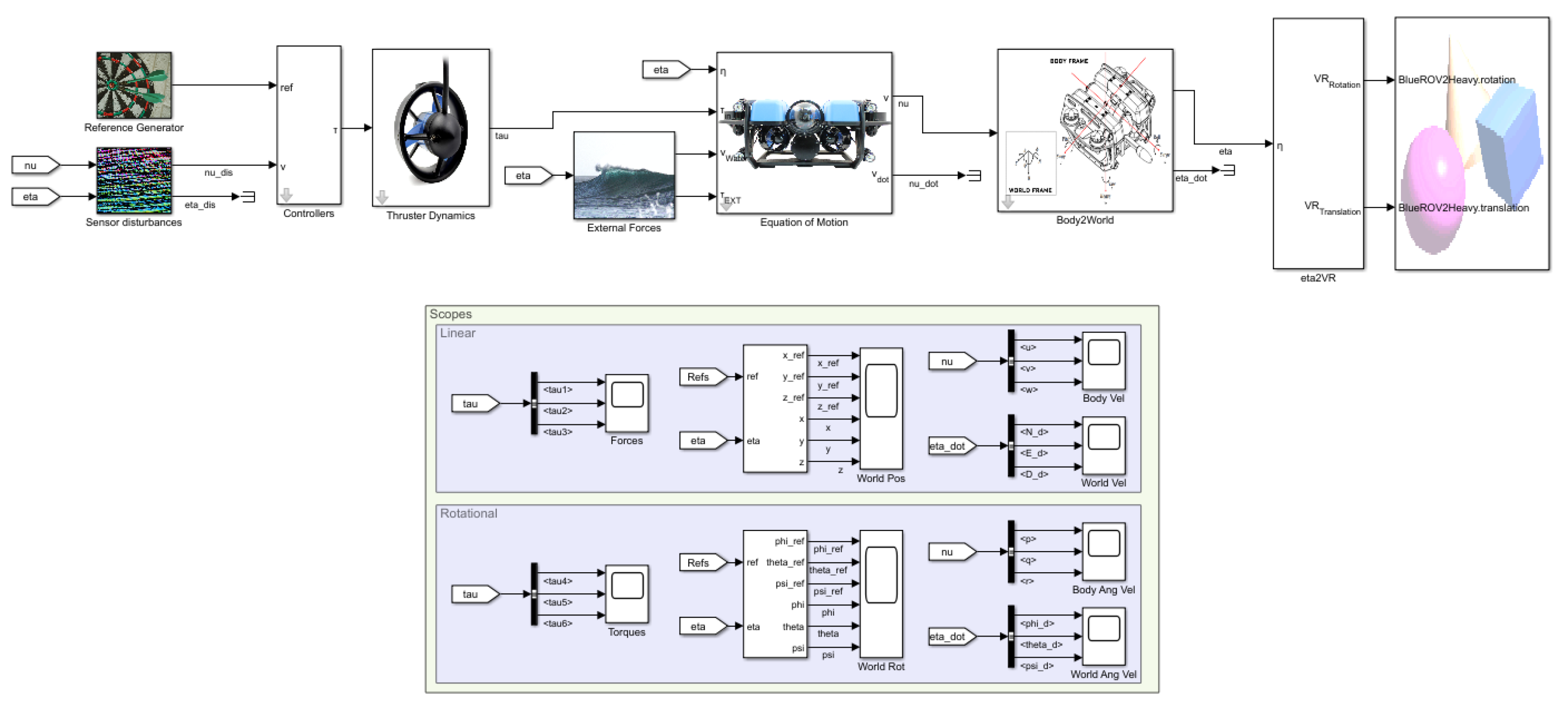
8. Simulator

The model of the BlueROV2 is found in Section 2, and together with the parameters found in Section 4 and the tether model found in Section 6 is implemented in a MATLAB™ and Simulink™ model. The controllers from Section 7 are also implemented for all six degrees of freedom. The behavior of the BlueROV2 is visualized with a simple 3D graphic environment, which is implemented in the simulator. 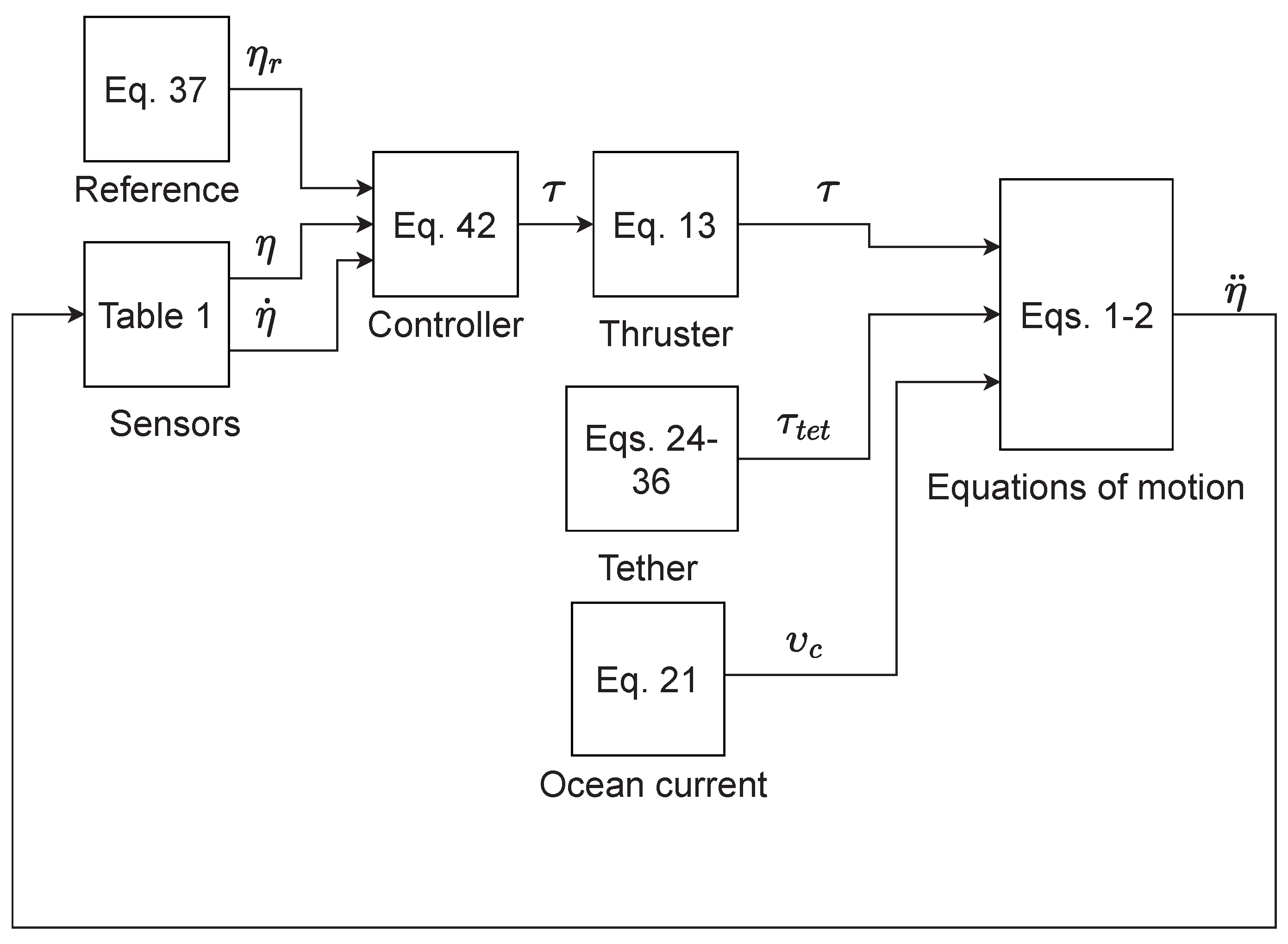The simulator will be demonstrated in a case study in Section 9. A simple block diagram of the simulator is shown in Figure 11, it shows how the equations of this paper are implemented in the simulator. 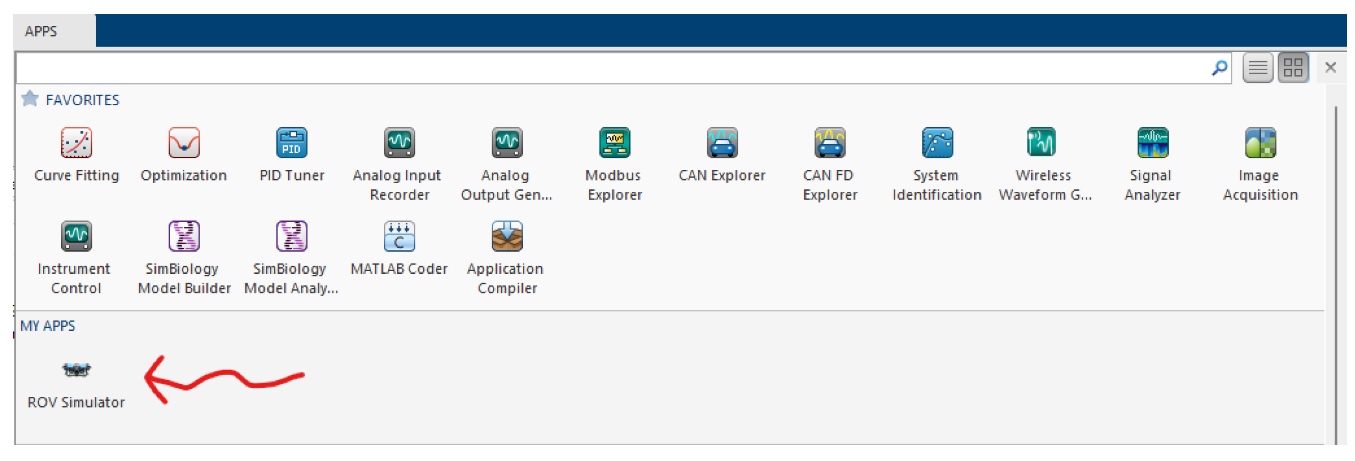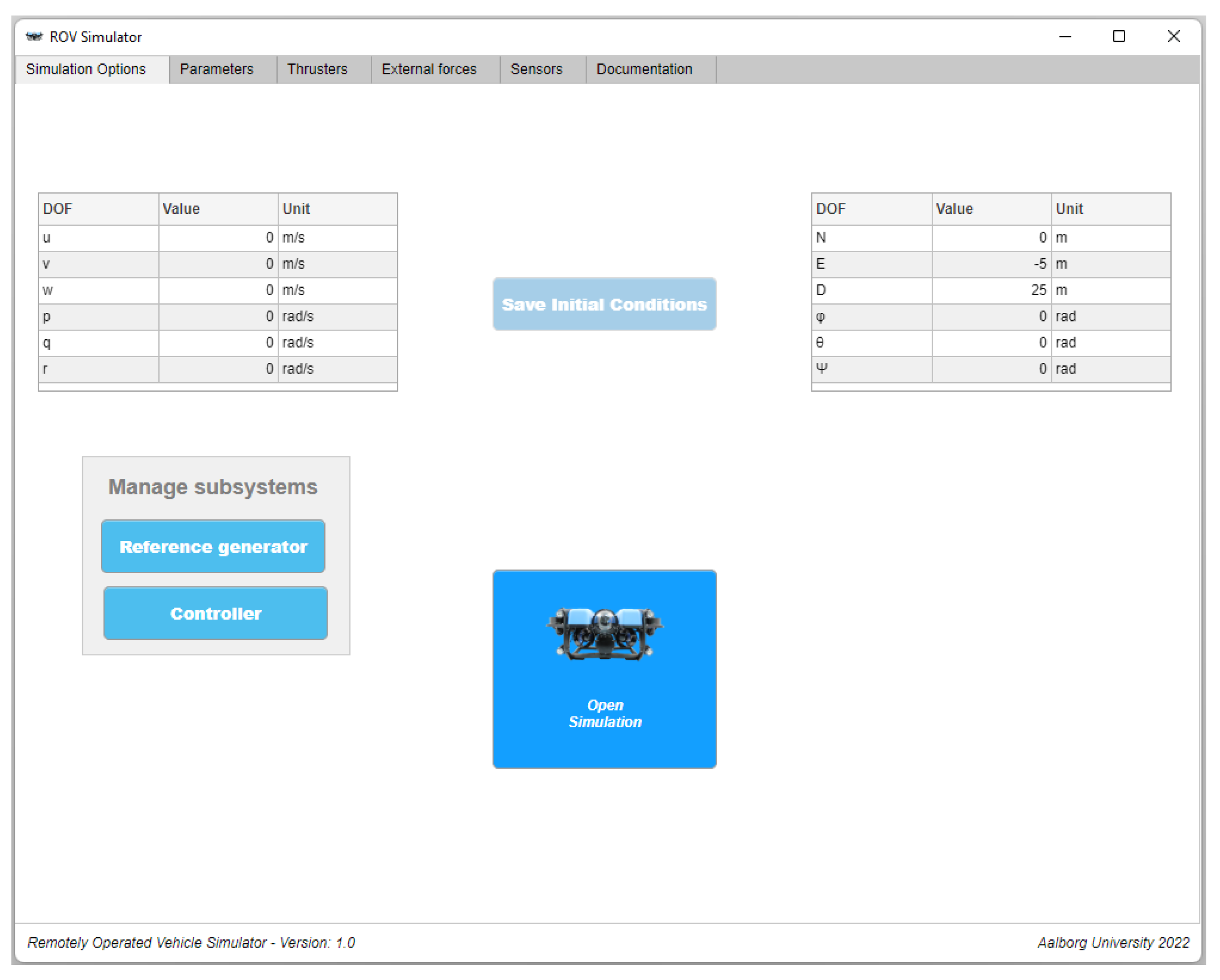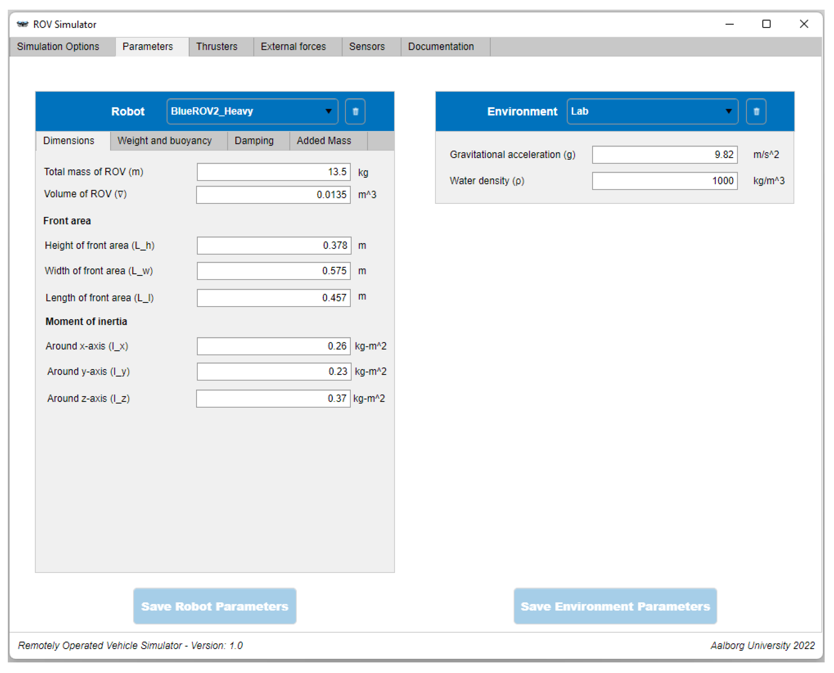A video of the simulator can be found in the attached files “Case study of simulator” or at Github in Supplementary Materials. The simulator will be updated occasionally. An implicit solver is recommended due to stiffness in the system of equations, e.g., ode15s in Simulink™. A detailed guide going through each step of setting up the simulator can be found in Appendix B.

9. Case Study-Offshore Mono Pile Inspection

In the this section, a case study will be carried out to demonstrate the simulator. Subsea inspections are a necessity in a variety of applications, such as in the oil and gas industry and the offshore wind industry. The case study will be based on an inspection of a monopile. The monopile is based on a realistic offshore wind turbine foundation of 6 m in diameter placed at depth of 25 m [39].

Offshore wind turbine operators have to account for a layer of marine growth when designing foundations for the offshore wind turbines, this increases the amount of steel used per installation [19]. An alternative to over-sizing the foundation is to remove the marine growth, so that it does not reach a thickness that is damaging to the structural integrity. The oil and gas operators to avoid an increase in surface area, which would decrease the fatigue life of the structure by cleaning the offshore structures periodically. However, cleaning requires annual inspections of the structure both before and after a cleaning job [40]. Before a cleaning job, inspections are needed to estimate the thickness of the marine growth to determine if it has reached a critical level, after a cleaning job inspections are carried out to verify that the marine growth has been removed and to inspect the structure for cracks to determine the structural integrity [19]. Wind turbine foundations that have been designed to withstand the marine growth layer must also be inspected for cracks, which in some cases also requires cleaning [40].

9.1. Design Criteria

The criteria for a successful inspection is for the ROV to take a picture at steps of one meter along the depth of the monopile with a relative distance of one meter between the camera and the monopile. The camera will be mounted along the surge direction in the ROV’s b-frame. The control parameters for the SMC has been designed according to Section 7.1, and can be seen in

Table 6. Tuned control parameters for SMC.

Controller	$\mathit{\alpha }$	${\mathbf{C}}_0$	${\mathit{ϵ}}_{\mathit{s}}$	${\mathbf{L}}_{\mathbf{b}}$
Surge	0.5	3	0.03	1.17
Sway	0.5	3	0.03	1.04
Heave	0.1	2	0.05	0.70
Roll	0.1	0.4	0.1	2.01
Pitch	0.1	0.4	0.1	1.83
Yaw	0.1	2	0.1	2.05

. The control parameters has been tuned initially based on simulations and then re-tuned from experimental data [3]. The noise variances and time delays in the feedback of the simulation will based on a DVL (u,v,w), a laser and camera (x,y), an IMU ($\varphi ,\theta$,p,q), a magnetometer ($\psi$,r) and a pressure sensor (z), see Table 1. The thruster allocation matrix in Section 3 is implemented in the simulation, but has not been considered in the control design.

The trajectory that the ROV will follow is shown in Figure 12. It is calculated based on

Table 7. Parameters for planning the campaign.

Description	Value	Unit
Diameter of the monopile	6	m
Distance to monopile	1	m
Camera angle	$2.09$	rad
Height of monopile	25	m
Inspection range	5–25	m
Velocity of the ROV	$0.2$	ms${}^{-1}$

. The initial conditions of the ROV, water current, and tether length can be seen in

Table 8. Tether and ROV parameters.

Description	Value	Unit
Initial position $(x_i,y_i,z_i)$	$[0,-5,25]$	m
Initial orientation (${\varphi }_i,{\theta }_i,{\psi }_i)$	$[0,0,0]$	rad
Current velocity	$[0.21,0.21,0]$	ms${}^{-1}$
Initial velocity of the ROV	$[0,0,0]$	ms${}^{-1}$
Initial angular velocity of the ROV	$[0,0,0]$	rads${}^{-1}$
Length of tether	35	m

. Note that the trajectory is not optimally designed, thus the ROV will not follow the shortest path.

9.2. Simulation Results

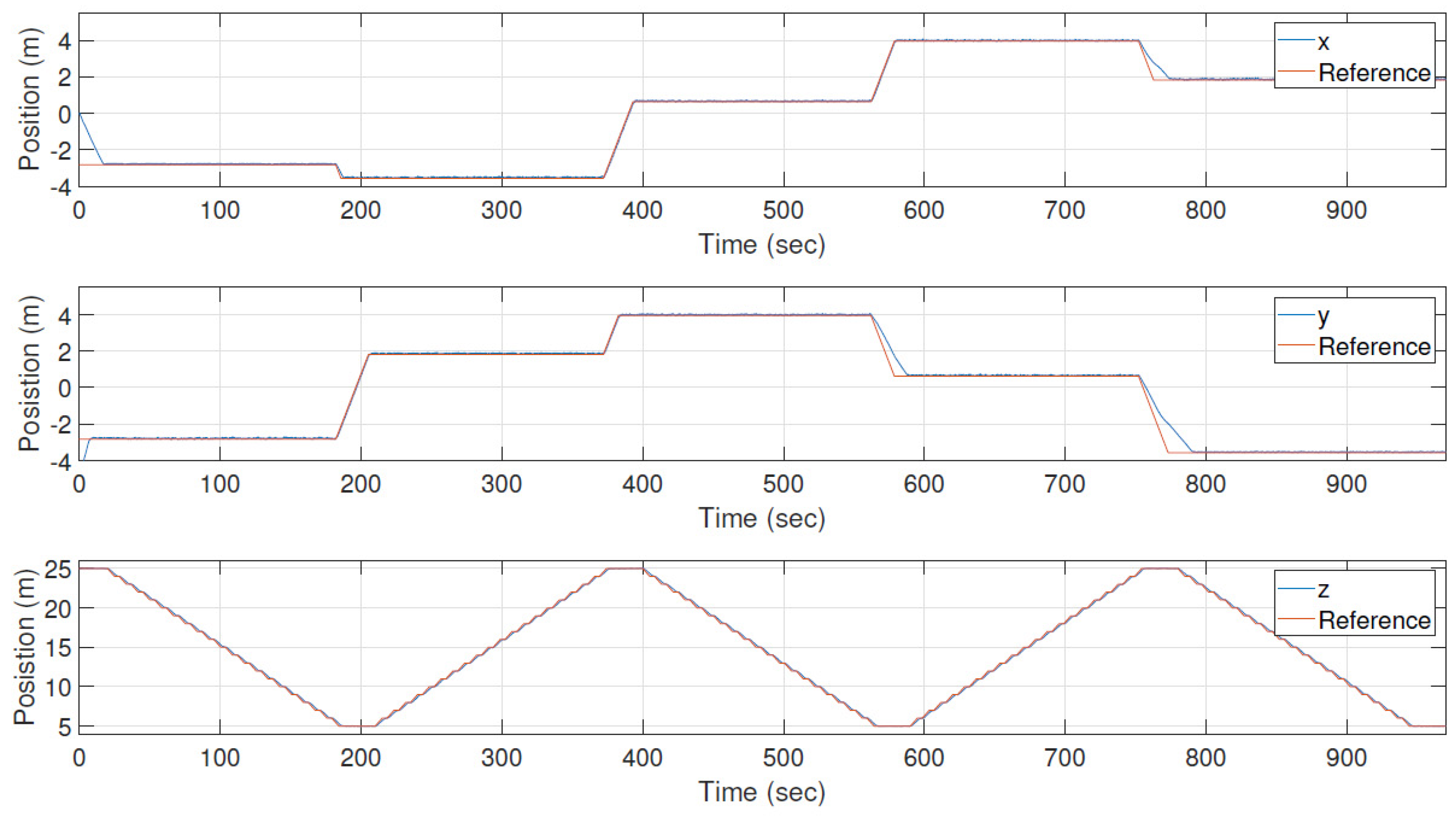
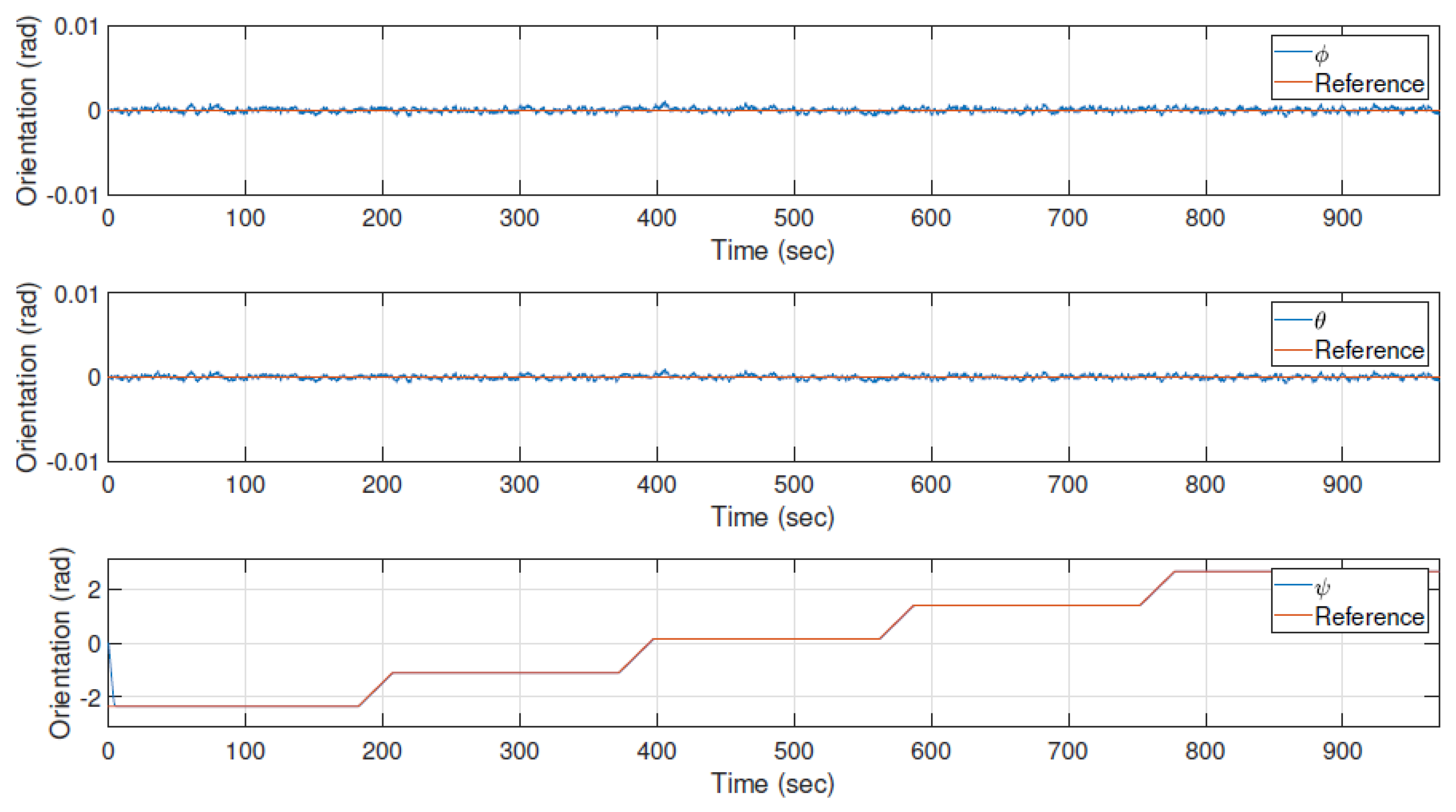
In this section, a brief overview of the simulation results from the case study will be presented. The pose, $\mathbf{\eta }$, of the ROV is seen in Figure 13 and Figure 14. The controller is able follow the trajectory with a low error, even though the ROV is influenced by the tether forces shown in Figure 15, the water current, a delay of 0.1 s in x and y from the DVL and the sensor noises. The ROV is initialized away from the trajectory to show that the controller is able to stabilize the ROV on the trajectory before it starts the mission. The starting point of the trajectory is at [$-2.83,-2.83,25,0,0,-0.75$ pi] with respect to the n-frame. The controller stabilizes the ROV at the reference within 20 s. Afterwards the ROV follows the trajectory, where it takes a picture at an interval of one meter in depth, from the bottom of the structure to 5 m below the surface. 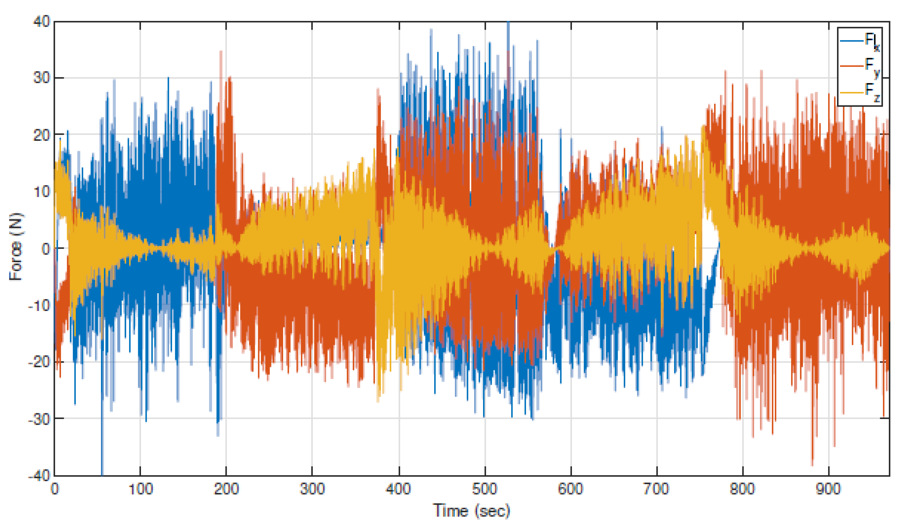From Figure 13, it can be noted that the controller has a difficulty following the trajectory when the ROV is moving in the negative x and y directions, this is caused by the ocean current pushing the ROV and tether in the opposite direction. There is a similar helping effect when the ROV moves in the positive x and y direction. In Figure 15, the tether force is shown, and it should be noted that the force fluctuates due to the interaction between the actively controlled ROV and the tether. Similar fluctuations are not seen in Figure 9, where the ROV is only acting as a passive weight. In

Table 9. Average and maximum tether forces during the inspection campaign. The number in parentheses is the percentage of the maximum thrust force.

Motion	Average of the	Average of the 5% Largest
	Absolute Forces	Absolute Forces
x	21.1 N (25%)	31.9 N (38%)
y	19.3 N (23%)	28.7 N (34%)
z	12.2 N (10%)	21.2 N (18%)

, an average of the absolute force and an average of the 5% largest forces are displayed. The impact from the tether is analyzed as statistical forces for each direction and given as a percentage of the maximum thrust force in that direction. For example, the ROV uses 38% of the thrust power to compensate for the 5% largest forces. It should be noted that this percentage is the ideal case since the ROV uses the same thrusters to surge and sway.

10. Concluding Remarks

This paper presented a dynamic BlueROV2 Simulator including a model of the tether connecting the ROV to the surface. The simulator is published in a MATLAB™ and Simulink™ environment. The simulator is designed to be used by the control community as a digital platform to implement control algorithms on and benchmark control algorithms. The dynamic model of the BlueROV2 is built on Fossens equations for underwater vehicles, which are widely used to model similar robotic platforms. The parameters have been found and validated using a combination of CAD software and physical experiments. The tether has been modeled using a lumped-mass approach which is an approximation of the standard finite element method. The tether model is included as it has a large impact on the dynamics of the ROV and is a necessity to do missions requiring large data transmissions, such as video feedback. A case study is presented where the ROV is deployed to inspect a monopile structure, and sliding mode control is implemented in the simulator to fulfill the task. The case study demonstrates the usefulness of the BlueROV2 simulator and the results establish a benchmark for future control schemes for positioning and orientation trajectory tracking. The simulator has been designed to be general purpose and all parameters can be changed in the App in MATLAB™ to fit a specific vehicle. It is possible to add additional blocks in the simulator for more advanced missions such as obstacle avoidance, optimal trajectory tracing, etc. Furthermore, additional disturbances can be added by applying the force to Equation (2), this could be water waves for vehicles working close to the surface or a reaction force from a tool.