Assessment of Ship Fuel Consumption for Different Hull Roughness in Realistic Weather Conditions

Abstract

This paper presents the effect of hull roughness over 10 years of operation on ship performance. The numerical model is developed by coupling NavCad and Matlab to perform the computation and the data processing. On the basis of a given hull, an engine, and an optimized propeller, the performance of the ship is computed for eight cases of hull roughness according to the ITTC recommendations in both calm waters and different weather conditions along the ship route. The effect of both wind and waves is considered for computing the added ship resistance along the route, thus requiring more power than just only the added resistance in waves. This provides a more accurate estimation of the ship’s performance along the different sea states. Lastly, a weighted average of the main ship parameters is estimated to evaluate better the ship’s performance. According to this study, the fuel consumption in calm water can be increased by around 20% after 10 years of ship operation based on the level of hull roughness. However, in the same weather conditions along the ship route, the ship’s fuel consumption can be increased by 10% compared to the same trip with a clean hull.

1. Introduction

The concept of green shipping has been applied to ensure a reduction in emissions along the ship route while using different types of resources and energy during the process of transportation [1,2,3]. This concept covers different aspects of the ship’s life, starting from the design procedure until reaching the ship’s operation to reduce the amount of fuel consumption significantly and, thus, increase the ship’s energy efficiency [4,5,6,7,8]. Therefore, the International Maritime Organization (IMO) has made an effort to stimulate the transition toward green shipping by applying stringent regulations to reduce the total annual greenhouse gas (GHG) by at least 50% by 2050 [9].

The ship hull form is one of the main aspects that need more attention when generating the hull lines to reduce the ship’s total resistance [10,11,12]. The starting point is to reduce ship resistance in calm water [10,13,14,15], but ship performance needs to account for the added resistance in waves [12,16,17,18] which is another major aspect in the design of the hull form.

More recently, computational fluid dynamics (CFD) methods have been used to determine ship resistance, which allows a detailed assessment of the effect of hull form, but also requires that the uncertainty in the predictions be properly accounted for [19,20,21].

Therefore, operation research techniques have been coupled to 3D software to benefit from the accuracy of the machine to predict the optimal solutions. For instance, Tezdogan et al. [22] developed a model coupling CFD and a nonlinear optimizer to reduce the ship resistance for a constant displacement and at a defined speed by finding the optimal parameters of a fishing boat. Seok et al. [23] used the design of experiments (DoE) and CFD methods to improve the bow shape of a tanker. As a result, the added resistance was reduced by 52% when compared to the original hull.

When predicting the resistance and propulsion of ships in seaways, both components of resistance need to be considered [24,25,26,27,28]. The effect of performance in seaways is very much related to fuel consumption [29,30], but also has consequences related to emissions [11,31,32] which are important not to avoid.

The performance of ships in seaways is also related to other operational aspects, such as the draught and trim of the ships [33,34,35] and the influence of wind [36,37]. As it is very difficult to properly account for all factors in a predictive model, many approaches have opted to address voyage data to derive global properties [38,39]. Furthermore, improving performance in voyages depends on avoiding heavy weather, which requires more power from the engines and leads to higher fuel consumption and emissions, which has promoted the wider use of weather routing approaches [40,41,42].

In addition to the optimized hull form, as the main concern of the ship designers during the design and building stages, the cleanliness and maintenance of the hull along the ship life are essential to keep the ship within the limits of consumption during operation. A 100,000 DWT tanker was studied by Smith and Colvin as an example [43], showing an increase in ship resistance by 30% due to biofouling, which leads to an increase in fuel consumption of 12 tons/day. Daidola [44] reported the causes of hull roughness, such as fouling, plate roughness, coating type, corrosion, and mechanical damage. The level of hull roughness can be determined using a hull roughness analyzer or by performing speed trials according to the material of coatings [45]. The level of average hull roughness (AHR) can increase by 2.3 to 12.8 μm per year according to the analysis of statistics vessel data for each dry dock event [46]. Therefore, the hull-cleaning process will be cost-effective and robust in the future using unmanned underwater vehicles, as reported by Song and Cui [47].

Several papers have simulated the performance of the ship in several roughness levels. Two methods have been used; the common one is CFD, although it has some uncertainties in the computed results [19], while the other is based on empirical formulas.

Regarding CFD methods, Haase et al. [48] predicted ship resistance by comparing CFD with experimental tests. They considered the hull roughness during the computation and reported higher values than the standard values reported by the International Towing Tank Conference (ITTC). Demirel et al. [49] used CFD to predict the effect of biofouling on ship resistance and power. According to the level of slime, they reported an increase in ship power by 18% to 38%. Yuan et al. [50] found that the viscous pressure and wave-making resistance are increasing more than the frictional resistance due to the roughness of the hull. Therefore, they suggested that the ship operates at lower speeds to reduce drag until it is cleaned. Song et al. [51] investigated the effect of biofouling on ship resistance and propulsive coefficient. They found that the frictional resistance was increased by up to 93%, while the wake fraction was increased by up to 47%, and both terms directly affected the ship speed.

Farkas et al. [52] demonstrated that the effect of biofilm could not be ignored as the ship speed was reduced by 2 knots, and the delivered power was increased by 36.3%. Song et al. [53] studied the effect of roughness on the hull and propeller and found that the total resistance coefficient can be increased by 52%, while the relative rotative efficiency and open water efficiency can be decreased by up to 2.6% and 20.1%, respectively. García et al. [54] used CFD to predict the total ship resistance of the ship for several years after validating the model used. They concluded that using CFD is an effective tool for studying biofouling’s effect on the ship hull. Sanz et al. [55] suggested that ceramic glaze can reduce the effect of biofouling and the resistance coefficient after 1 year by 80% compared to conventional paints. Islam et al. [36] used OpenFoam as a CFD tool to simulate the aerodynamic load of a fast ship, showing good agreement with the experimental data.

Regarding empirical equations and using the generated diagrams to compute the added resistance due to fouling, as well as the power losses, Demirel et al. [56] estimated the new resistance for different types of ships, and the method showed its ability to be applied to any kind of ships with length varying from 10 m to 400 m. Uzun et al. [57] used a time-dependent model to predict the level of biofouling while analyzing the ship’s performance during operation. The model developed can predict the optimal time to perform the ship’s maintenance.

According to the literature review, this paper contributes to computing the ship performance, engine loading, and fuel consumption along a specific route, comparing the results over 10 years of operation due to the different levels of hull roughness. First, on the basis of an optimized propeller geometry previously predicted by Tadros et al. [58], the ship’s performance is computed in calm water for a different level of roughness based on ITTC equations. Then, the weighted average of ship performance is simulated along the ship route from the European Union (EU) to the United States (USA) for different weather conditions and according to the occurrence of the sea state, where the added resistance due to wind and wave is considered during the simulation.

The remainder of this paper is organized as follows: first, the numerical model used to perform the simulation is presented in detail in Section 2. Next, the computed results and the evaluation of the ship, engine, and propeller performance in both calm water and different weather conditions are presented in Section 3. Lastly, a summary of the main findings and recommendations for future work are presented in Section 4.

2. Numerical Model

The ship selected to perform the computation is a bulk carrier operating between EU and USA through the Atlantic ocean [59]. This ship has 154 m in length and is equipped with a four-stroke marine diesel engine at 7140 kW to allow the ship to sail at 14.5 knots. The ship can reach up to 16 knots at maximum power. The ship is equipped with a single fixed-pitch propeller (FPP) with a 6 m diameter. This propeller was selected using an optimization procedure previously developed in [58], coupling NavCad from HydroComp [60] and a nonlinear optimizer integrated into Matlab to design the propeller at the engine operating point with minimum fuel consumption. This model has shown its effectiveness in computing the propeller performance in different applications [61,62,63]. For instance, the contra-rotating propeller can lead to a more than 10% reduction in fuel consumption [64]. The propeller was selected by considering the smooth hull (zero roughness) as commonly known in the design procedures. The propeller was selected after computing the total resistance of the ship hull using the methods presented in [65,66] that showed effectiveness compared with CFD [67], and then the wake fraction (w), thrust deduction factor (t), and relative rotative efficiency (η_RR) as propulsive coefficients were computed using the methods presented in [68]. The main characteristics of the ship, engine, and propeller are given in Table 1.

The total resistance of the ship is composed of the total resistance in calm water, the added resistance due to waves and wind, and a specific margin depending on the design stage. The last element is a percentage of the total hull drag and the added drag. In this study, 10% was selected as a feasible design margin. The total resistance in calm water was computed using the following expression based on the methods presented in ITTC-78 [69].

$${\mathrm{C}}_{\mathrm{T}}{=(1+\mathrm{k})\mathrm{C}}_{\mathrm{F}}{+\mathrm{C}}_{\mathrm{R}}{+\mathrm{C}}_{\mathrm{A}}{+\mathsf{\Delta }\mathrm{C}}_{\mathrm{F}}$$

(1)

where C_T is the total resistance coefficient, k is the hull form factor computed using the Holtrop method as mentioned in ITTC-57 [70], C_R is the residuary resistance coefficient, C_A is the correlation allowance, and ∆C_F is the roughness allowance computed using the following expression:

$${\mathsf{\Delta }\mathrm{C}}_{\mathrm{F}}=0.044\left[{\left(\frac{{\mathrm{k}}_{\mathrm{s}}}{\mathrm{LWL}}\right)}^{\frac{1}{3}}{–10\mathrm{Re}}^{\frac{–1}{3}}\right]+0.000125$$

(2)

where k_s is the roughness of the hull surface as defined by the designer, LWL is the ship length at the water line, and Re is the Reynolds number.

The added resistance was computed on the basis of realistic weather conditions along the ship route, consisting of the added resistances due to waves and wind; each component was computed separately.

Table 1. Main characteristics of the bulk carrier.

	Characteristics	Symbol	Unit	Value
Ship characteristics	Length at waterline	LWL	m	154.00
	Breadth	B	m	23.11
	Draft	T	m	10.00
	Displacement	∆	tonne	27,690
	Service speed	Vs	knot	14.5
	Maximum speed	Vs-max	knot	16.0
	Number of propellers	-	-	1
	Type of propellers	-	-	FPP
	Rated power	Pmax	kW	7140
Engine characteristics	Engine builder	-	-	MAN Energy Solutions [71]
	Brand name	-	-	MAN
	Bore	B	mm	320
	Stroke	S	mm	440
	Displacement	V	liter	4954
	Number of cylinders	nc	-	14
	Rated speed	RPMmax	rpm	750
	Rated power	Pmax	kW	7140
	Speed at 14.5 knots	RPM	rpm	714
Propeller characteristics	Series	-	-	Wageningen B-series
	Diameter	D	m	6
	Expanded area ratio	EAR	-	0.47
	Pitch diameter ratio	P/D	-	1.097
	Gearbox ratio	GBR	-	9.5
	Number of blades	Z	-	5
	Speed at 14.5 knots	N	rpm	75

Table 1. Main characteristics of the bulk carrier.

	Characteristics	Symbol	Unit	Value
Ship characteristics	Length at waterline	LWL	m	154.00
	Breadth	B	m	23.11
	Draft	T	m	10.00
	Displacement	∆	tonne	27,690
	Service speed	Vs	knot	14.5
	Maximum speed	Vs-max	knot	16.0
	Number of propellers	-	-	1
	Type of propellers	-	-	FPP
	Rated power	Pmax	kW	7140
Engine characteristics	Engine builder	-	-	MAN Energy Solutions [71]
	Brand name	-	-	MAN
	Bore	B	mm	320
	Stroke	S	mm	440
	Displacement	V	liter	4954
	Number of cylinders	nc	-	14
	Rated speed	RPMmax	rpm	750
	Rated power	Pmax	kW	7140
	Speed at 14.5 knots	RPM	rpm	714
Propeller characteristics	Series	-	-	Wageningen B-series
	Diameter	D	m	6
	Expanded area ratio	EAR	-	0.47
	Pitch diameter ratio	P/D	-	1.097
	Gearbox ratio	GBR	-	9.5
	Number of blades	Z	-	5
	Speed at 14.5 knots	N	rpm	75

The added resistance due to waves was computed on the basis of the defined significant wave height (H_W) and the modal wave period (T_P) according to the position of the ship along the route, following Aertssen’s [72] method. This method is integrated into NavCad and is based on the ship’s volume and the characteristics of the sea state. The main advantage of this method is that it does not account for ship type and the method in NavCad is modified from the original one to extract the added resistance due to wind from the computation and compute only the added resistance due to the waves.

The added resistance due to wind was computed by defining the characteristics of the wind to which the ship is subjected, such as speed and direction. Furthermore, the total areas of the exposed hull and the superstructure were defined from the 3D model of the selected ship. The method proposed by Taylor [73] was used in this study as it is based on tanker, cargo ship, and passenger liner models where the pseudo-drag coefficients are considered according to empirical testing, and the total added resistance due to wind (R_wind) was computed using the following expression.

$${\mathrm{R}}_{\mathrm{Wind}}=\frac{1}{2}\mathrm{CA}{\rho }_{air}{\mathrm{V}}^2$$

(3)

where C is the drag coefficient, A is the affected area of the hull and superstructure, ρ_air is the mass density of the air, and V is the ship speed.

The propeller performance was computed on the basis of the advance coefficient (J_A), thrust coefficient (K_T), torque coefficient (K_Q), and the propeller efficiency (η_o), as presented in the following expressions [74]:

$${\mathrm{J}}_{\mathrm{A}}=\frac{{\mathrm{V}}_{\mathrm{A}}}{\mathrm{nD}}$$

(4)

$${\mathrm{K}}_{\mathrm{T}}=\frac{\mathrm{T}}{{\rho }_w{\mathrm{n}}^2{\mathrm{D}}^4}$$

(5)

$${\mathrm{K}}_{\mathrm{Q}}=\frac{\mathrm{Q}}{{\rho }_w{\mathrm{n}}^2{\mathrm{D}}^5}$$

(6)

$${\mathsf{\eta }}_{\mathrm{o}}=\frac{{\mathrm{K}}_{\mathrm{T}}}{{\mathrm{K}}_{\mathrm{Q}}}\frac{{\mathrm{J}}_{\mathrm{A}}}{2\mathsf{\pi }}$$

(7)

where V_A is the advance speed, n is the propeller speed, ρ_w is the water density, T is the propeller thrust, and Q is the propeller torque.

The cavitation was evaluated on the basis of several criteria showing a good combination to ensure the reliability of the propulsion system. The first was the method proposed by Keller [75], where the expanded area ratio is to be greater than the minimum one computed from the developed equation. Second, the average loading pressure must be less than 65 kPa, as computed from the Burrill chart [76]. Third, the average predicted back cavitation percentage must be less than 15%, according to Blount and Fox [77]. Fourth, the propeller pitch must be greater than the minimum pitch computed by MacPherson [78], avoiding face cavitation. Lastly, the tip speed must be less than 46 m/s for this five-blade propeller [60].

The propeller geometry was selected along with the GBR, which was kept constant and selected depending on the engine’s speed and the propeller’s speed. The efficiencies of the gearbox and propeller shaft were taken into account, assumed as 97%.

Subsequently, the propeller performance was implemented into the engine load diagram, and the fuel consumption was computed as a function of the brake specific fuel consumption (BSFC) according to the computed results of engine performance shown in [79,80].

$${\mathrm{FC}}_{\mathrm{kg}/\mathrm{nm}}=\frac{\mathrm{BSFC} \times { \mathrm{P}}_{\mathrm{B}}\times 1000}{{\mathrm{V}}_{\mathrm{S}}}$$

(8)

where P_B is the brake power.

Following the concept presented in [81], the engine power limitation technique was applied. A correction procedure of the operating point along the propeller curve was performed when the propeller operating point exceeded 90% of the rated engine power, and speed losses were calculated. Moreover, a weighted average technique was applied to evaluate the performance of the ship and the amount of fuel consumption along the route by considering the number of occurrences of each sea state along the trip. The weighted average of each parameter was computed using the following expression:

$${\mathrm{P}}_{\mathrm{W}}=\frac{{\displaystyle \sum _{\mathrm{i}=1}^{\mathrm{n}}{\mathrm{P}}_{\mathrm{i}}\times \hspace{0.17em}{\mathrm{SS}}_{\mathrm{Occ},\mathrm{i}}}}{{\displaystyle \sum _{\mathrm{i}=1}^{\mathrm{n}}{\mathrm{SS}}_{\mathrm{Occ},\mathrm{i}}}}$$

(9)

where P_W is the weighted average parameter, P is the specific parameter, SS_Occ is the occurrence of the sea state, and n is the number of sea states.

The simulation process along the ship route is very complex when performed manually due to the large number of simulations; however, due to the application programming interface (API), the processing of data and computation of the model become easier and faster. After the optimization procedures of the propeller selection in the engine load diagram were performed by minimizing the fuel consumption in calm water conditions, the ship’s performance was processed in the weather conditions (wave only; wave and wind).

This process was performed in two steps for comparison of the methods used; the first step was to compute the added resistance due to waves only, and then the second step was to compute the added resistance due to wind while keeping the added resistance due to waves computed in the previous step. This process allows data extraction at a suitable time according to the selected method of added resistance. The simulation process is detailed in the schematic diagram in Figure 1.

3. Results

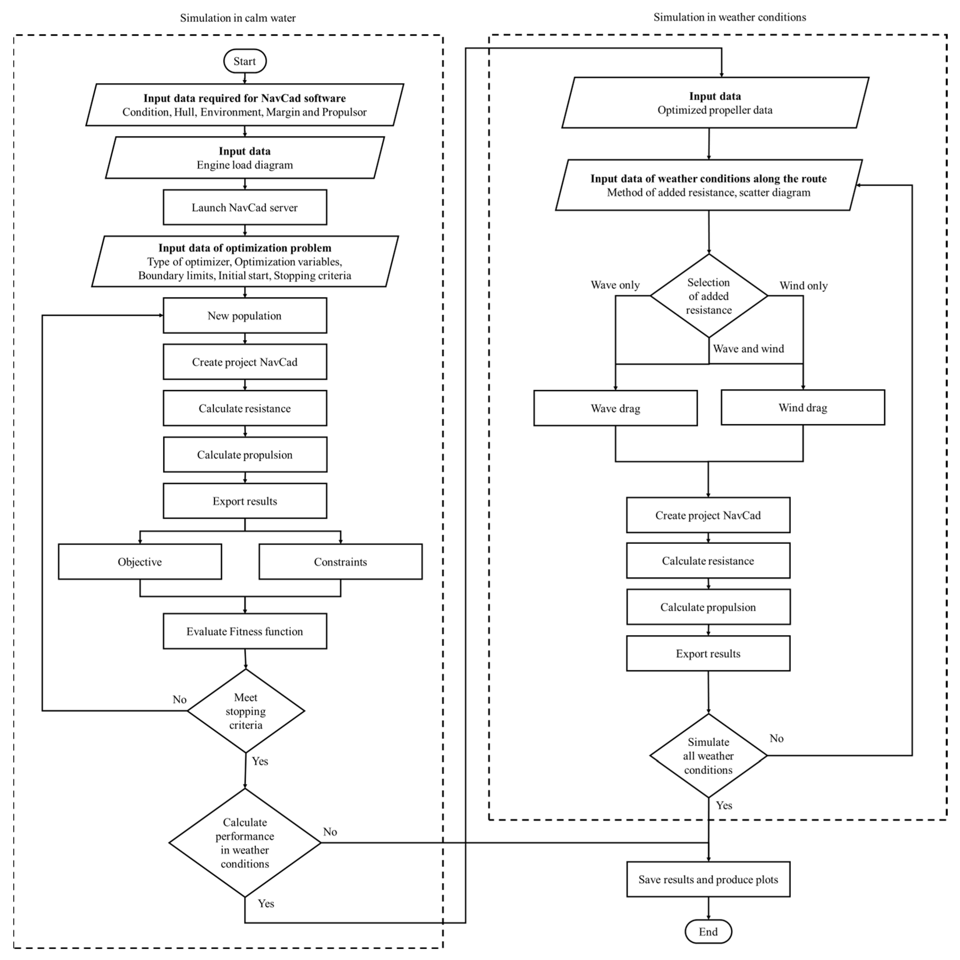
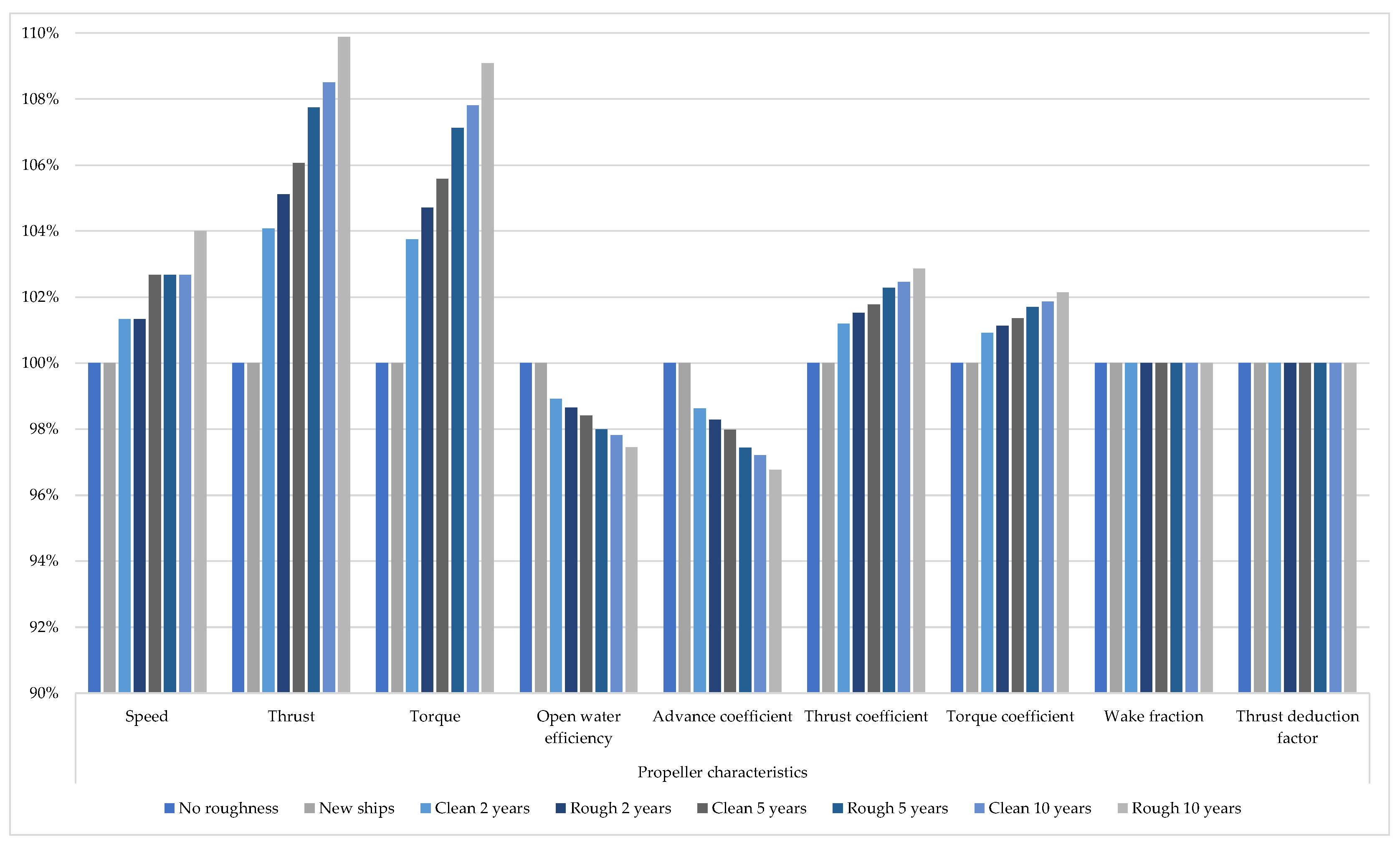
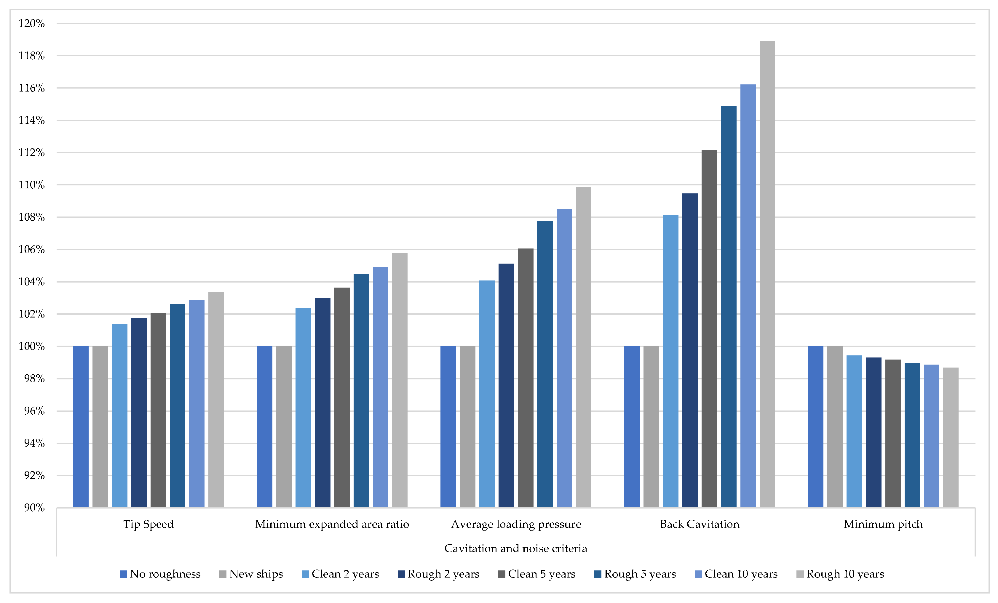
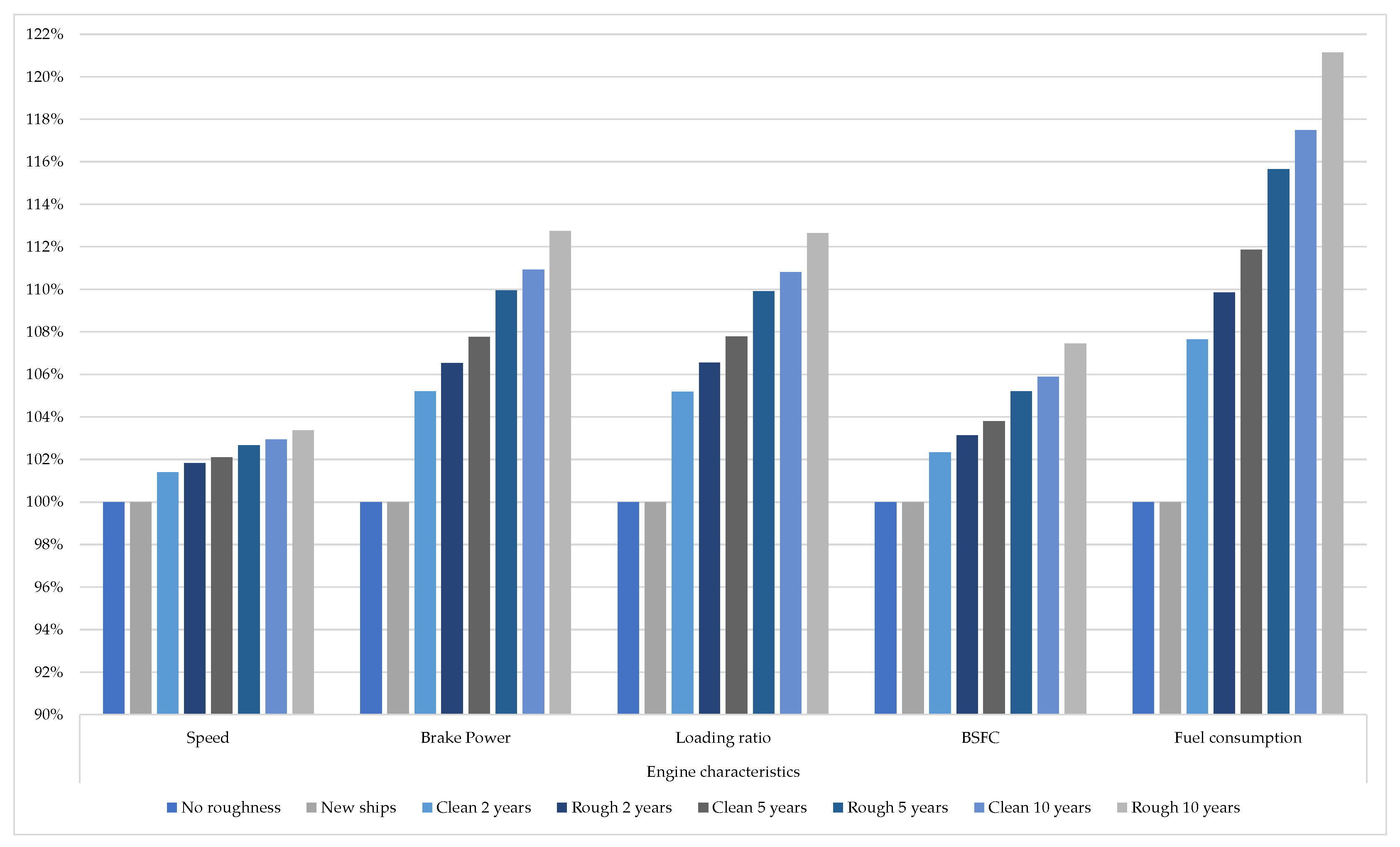
3.1. Simulation in Calm Water

After the establishment of the model and the optimization procedure were performed, the propeller geometry and the gearbox ratio were selected for zero roughness. Then, on the basis of the optimized parameters, the propeller and engine performance were simulated while changing the value of the hull roughness. Eight cases were computed for performing the comparison and predicting the change in system performance as follows: (1) no roughness (0 mm), (2) new ships (0.15 mm), (3) clean ship after 2 years (0.3 mm), (4) rough ship after 2 years (0.35 mm), (5) clean ship after 5 years (0.4 mm), (6) rough ship after 5 years (0.5 mm), (7) clean ship after 10 years (0.55 mm), (8) rough ship after 10 years (0.65 mm). The roughness values were selected according to the recommendations of the ITTC [82] due to the fouling and deterioration of the hull over the years. The chosen roughness values show that there was no escape from the increment in the roughness values over the years, which would affect the ship’s performance. The actual data are presented in

Table A1. Optimum results for different configurations.

Main Characteristics	Parameters	Unit
Level of Roughness			No roughness	New ships	Clean 2 years	Rough 2 years	Clean 5 years	Rough 5 years	Clean 10 years	Rough 10 years
Roughness		[mm]	0.00	0.15	0.30	0.35	0.40	0.50	0.55	0.65
Ship characteristics	Ship speed	[kn]	14.5	14.5	14.5	14.5	14.5	14.5	14.5	14.5
Propeller characteristics	Series	[-]	Wageningen B-series
	Cup	[%]	0.00	0.00	0.00	0.00	0.00	0.00	0.00	0.00
	Diameter	[m]	6.00	6.00	6.00	6.00	6.00	6.00	6.00	6.00
	Expanded area ratio	[-]	0.47	0.47	0.47	0.47	0.47	0.47	0.47	0.47
	Pitch	[m]	6.58	6.58	6.58	6.58	6.58	6.58	6.58	6.58
	Speed	[RPM]	75.00	75.00	76.00	76.00	77.00	77.00	77.00	78.00
	Thrust	[kN]	576.5	576.5	599.9	605.9	611.5	621.1	625.5	633.5
	Torque	[kN.m]	573.3	573.3	594.8	600.3	605.3	614.1	618.1	625.4
	Open water efficiency	[%]	59.32	59.32	58.68	58.52	58.38	58.13	58.02	57.81
	Advance coefficient	[-]	0.62	0.62	0.61	0.61	0.61	0.60	0.60	0.60
	Thrust coefficient	[-]	0.28	0.28	0.28	0.28	0.28	0.28	0.28	0.28
	Torque coefficient	[-]	0.05	0.05	0.05	0.05	0.05	0.05	0.05	0.05
	Wake fraction	[-]	0.38	0.38	0.38	0.38	0.38	0.38	0.38	0.38
	Thrust deduction factor	[-]	0.19	0.19	0.19	0.19	0.19	0.19	0.19	0.19
Cavitation and noise criteria	Tip Speed	[m/s]	23.61	23.61	23.94	24.02	24.10	24.23	24.29	24.40
	Minimum expanded area ratio	[-]	0.47	0.47	0.48	0.48	0.49	0.49	0.49	0.50
	Average loading pressure	[kPa]	43.57	43.57	45.34	45.80	46.21	46.94	47.27	47.87
	Back cavitation	[%]	7.40	7.40	8.00	8.10	8.30	8.50	8.60	8.80
	Minimum pitch	[m]	4978.5	4978.5	4950.4	4943.4	4937.1	4926.2	4921.3	4912.5
Gearbox characteristics	Gearbox ratio	[-]	9.5	9.5	9.5	9.5	9.5	9.5	9.5	9.5
Engine characteristics	Speed	[RPM]	714	714	724	727	729	733	735	738
	Brake power	[kW]	4682.3	4682.3	4925.8	4988.6	5045.9	5147.9	5194.1	5278.9
	Loading ratio	[%]	65.6	65.6	69	69.9	70.7	72.1	72.7	73.9
	BSFC	[g/kW.h]	191.8	191.8	196.3	197.8	199.1	201.8	203.1	206.1
	Fuel consumption	[kg/nm]	61.93	61.93	66.67	68.04	69.29	71.64	72.77	75.02

, Appendix A for more information, while the percentage change for different parameters is presented in Figure 2, Figure 3 and Figure 4. The percentage change was calculated on the basis of the first case with zero roughness as a reference value.

Regarding the propeller characteristics, as presented in Figure 2, an increase in propeller speed along the simulated cases showed a maximum increment of 4% comparing the same ship in new conditions and rough conditions after 10 years. This increment in propeller speed was due to the increase in the thrust required to achieve the same ship speed (14.5 knots), which was increased by up to 10% comparing the first and the last cases. The propeller torque exhibited the same behavior, which increased with the increase in the level of roughness by up to 9% to provide the required thrust to the ship with a slight reduction in torque, while the advance coefficient was reduced when the propeller speed increased by around 3% comparing the same two cases.

This increment in thrust and torque directly affects the propeller coefficient, leading to increases the thrust and torque coefficients by 3% and 2%, respectively. According to these changes in propeller coefficients, the open water efficiency followed the same advance coefficient behavior and was reduced by about 2.5% over the 10 years. However, the wake fraction and thrust deduction factor were kept constant throughout the cases due to some limitations in the empirical formulas. These two factors required more detailed simulation-based CFD to be able to predict the accurate changes according to the hull roughness; however, there was no big difference detected in previous studies [83].

From the full results, the first and second cases presented similar results, showing that there was no effect when the roughness increased from 0 to 0.15 mm.

Regarding the cavitation and noise criteria, as presented in Figure 3, all criteria, except the minimum pitch, increased upon raising the level of roughness due to the increase in propeller speed and propeller thrust, which increased the pressure along the propeller blades. A 3.5% difference in tip speed was detected comparing the first and the last cases; however, this value increased for the other criteria, showing a maximum value of 19% in the back cavitation criterion.

The last criterion was reduced by up to 1.5% as a function of the advance coefficient, as presented in Equation 10, which was reduced due to the increase in propeller speed.

$${\left(\frac{\mathrm{P}}{\mathrm{D}}\right)}_{\min }=\frac{{\mathrm{J}}_{\mathrm{A}}{+\mathrm{J}}_{\mathrm{A}}\sqrt{\frac{2{.55\mathrm{K}}_{\mathrm{T}}}{{\mathrm{J}}_{\mathrm{A}}{}^2}+1}}{2}$$

(10)

While there was a big change in the values when the level of roughness increased, all the computed results were under the limits of cavitation except the minimum EAR, as detailed in Table A1 in Appendix A. However, it is essential to keep the hull clean, ensuring the safety of the ship and avoiding any kidding of corrosion over the years.

Regarding the engine performance, as presented in Figure 4, the engine speed increased proportionally to the propeller speed, where there was no change in the value of the gearbox ratio, in order to provide sufficient power to operate the ship at the same speed. The engine speed increased by around 3% over the 10 years.

Moreover, the brake power and the loading ratio increased by about 13% when the hull roughness increased over the 10 years. On the basis of these changes, the BSFC also increased according to the data provided from the engine load diagram, thus increasing the fuel consumption per nautical mile as the main parameter of interest in the maritime field. The fuel consumption increased by around 7.5% after 2 years for a clean hull, reaching 10% in a rough hull compared to a new hull. The fuel consumption increased by 12% for a clean hull and 15.5% for a rough hull after 5 years, while these values could reach 17.5% and 21% after 10 years for a clean and rough hull, respectively. Therefore, it is important to keep an eye on the maintenance of the submerged part of the hull.

3.2. Simulation in Weather Conditions (Wave and Wind)

After the ship’s performance was computed and the operational point of the propeller was defined inside the engine load diagram for different surface roughness, the next step was to compute the ship’s performance along the ship route in different wave conditions, followed by the corresponding wind conditions. The characteristics of the sea states along the ship route from the British Channel to the east coast of the USA were defined according to the H_W, which varied between 0 and 10 m, and the T_P, which varied between 4 and 18 s [59,84], while the variation of wind direction was computed on the basis of H_W, as presented in [85] in the winter season (DJF). The wind direction varied between 22° and 53° relative to the bow of the ship. Lastly, the wind speed was computed as an average value according to the Beaufort number as defined in the software.

The defined route is presented in Figure 5, and the scatter diagram of the selected route is shown in Figure 6.

On the basis of the computation procedure carried out, the percentage of added resistance due to waves and wind was computed for different surface roughness and sea state values along the ship route. The computed results revealed the amount of added resistance to operate the ship at the same speed (14.5 kn).

The percentage of each added resistance is presented as a percentage of the total resistance for each sea state in Figure 7. In this paper, the behavior of the added resistance of the ship was indicated in the case of a new ship, where the roughness was equal to 0.15 mm, and after 10 years of operation with a clean hull, where the roughness was equal to 0.55 mm.

The results show that the added resistance due to waves and wind had a big share of the total resistance in weather conditions, and the wind resistance must not be neglected during the computation to achieve an accurate result. It was shown that the added resistance due to waves and wind increased significantly with higher sea states and could reach around 45% of the total resistance. In lower sea states, the added resistance due to wind was dominant and slightly higher than that due to waves caused by the large area of the superstructure and hull profile above the water line. Furthermore, the wind speed was almost relative to the ship from the bow, which directly increased the wind resistance. This percentage was reduced for higher sea states with a significant wave height of more than 3.5 m, and the added resistance due to the wave became dominant. The percentage of added resistance due to the wave increased until reaching double the value in higher sea states than the wind resistance to achieve the required speed.

The same behavior of ship resistance was detected after 10 years of ship operation, where there was an increase in ship roughness. While there was an increase in ship resistance over the years, the percentages of added resistance due to waves and wind from the computed total resistance were almost the same.

The same behavior was detected when computing the amount of brake power required to operate the ship and achieve the required speed. The amount of variation in the increase in brake power is presented in Figure 8, where the increase in brake power was computed in relation to the computed brake power in calm water. The increase in computed brake power was calculated for the ship as a new hull and after 10 years of operation. This brake power increment was to achieve the design speed, whereas, in real operation, there is always a reduction in sailing speed to ensure the safety of the propulsion engine from overloading.

The same behavior was detected for both cases, with a slight difference in brake power percentage. For instance, in lower sea states, the increase in brake power due to wind was slightly higher than due to wave, and this value was reduced with higher sea states, where the amount of brake power required for wave resistance was double that for wind resistance. These computations were performed without any engine power limitation or speed reduction to study the ship’s behavior in the different sea states. These types of analyses show the percentage increase in ship resistance and the brake power required for both components to achieve the same speed, showing that the brake power could be increased by 100% in lower sea states and by 50% in higher sea states to achieve the design speed.

By applying a speed reduction technique in real operation to prevent the engine from overloading, thereby reducing the level of exhaust emissions from the ship during operation in high weather conditions and ensuring the safety of the ship, any operational point of the ship that exceeded 90% of the rated engine power was corrected, and the propeller point operated at 90% of the rated power. All the corrections regarding the ship speed were recalculated, and the speed losses were predicted, as shown in Figure 9 and Figure 10 for the new and 10 year old ships, respectively. It was detected that the ship began losing speed in the sea state with a significant wave height of more than 3.5 m and a modal wave period higher than 9 s. In the case of the new ship, the percentage of ship losses could reach up to 18% of the design speed in high weather conditions, whereas, after 10 years, the speed losses could reach 21% of the design speed.

After computing the speed losses along the trip for different sea states, the cavitation of the propeller was evaluated on the basis of the various criteria mentioned previously.

Figure 11 shows the minimum EAR required to avoid cavitation. While the designed propeller complied with the limitations of the Keller method, it is shown that the propeller was exposed to cavitation along the ship route for the different weather conditions due to the increase in propeller thrust in sea states to achieve the ship speed. Furthermore, there was no margin between the EAR of the propeller and the required minimum EAR, as they were equal. A slight increase in the minimum EAR of the 10 year old ship was detected compared to the new hull. This was due to the increase in ship resistance over the years, which needed more thrust than the new hull.

Considering the average predicted back cavitation based on the Burrill method, as shown in Figure 12, the propeller had a lower probability of being exposed to the cavitation problem in lower sea states as the computed percentage was lower than the limits of cavitation. However, in higher weather conditions, particularly with a 5.5 m significant wave height or more, the percentage cavitation exceeded the limits, and propeller cavitation could occur. These values showed an increment for the 10 year old ship but still followed the same behavior, and propeller cavitation could occur in the same sea states.

Considering the average loading pressure shown in Figure 13, the same behavior as in the previous criteria was detected, where propeller cavitation could occur starting from the sea states with 5.5 m significant wave height or more. A slight increase in the value of this criterion was detected for the old ship.

Regarding the tip speed, as shown in Figure 14, the noise level produced by the propeller was under the maximum limits for the weather conditions along the ship route. Therefore, the ship could easily comply with this criterion whether the hull was new or old.

Lastly, the performance of the ship along the route was evaluated using the weighted average parameters as a function of the percentage of occurrence of each sea state. Figure 15 presents the variation of the main parameters of the ship, engine, and propeller for the different levels of hull roughness. Engine speed and power, ship speed, and the amount of fuel consumption were the main parameters used to evaluate the total performance of the ship. The actual data are presented in

Table A2. Comparison of the weighted average results for different roughness along the route.

Item (Weighted Average)	Unit
Level of Roughness	[-]	No roughness	New ships	Clean 2 years	Rough 2 years	Clean 5 years	Rough 5 years	Clean 10 years	Rough 10 years
Roughness	[mm]	0.00	0.15	0.30	0.35	0.40	0.50	0.55	0.65
Engine speed	[RPM]	755.22	755.22	761.18	762.37	763.70	765.83	766.96	768.66
Engine power	[kW]	5800.6	5800.6	5974.9	6016.4	6054.3	6121.7	6152.2	6208.2
Ship speed	[kn]	14.33	14.33	14.26	14.24	14.23	14.20	14.18	14.16
Fuel consumption	[kg/nm]	86.35	86.35	88.73	89.41	90.28	92.62	93.47	95.09

.

As previously mentioned, neglecting the effect of roughness and the new clean hull resulted in the same behavior regarding the main parameters, which can be considered the main reference compared to the other roughness levels. On the basis of the simulation of the whole trip, the weighted average engine speed was slightly increased in the considered cases, reaching 2% in the last case compared to the reference case.

The weighted average engine brake power increased along the cases, and a 7% increment was reached after 10 years of operation compared to the new hull. The weighted average ship speed was slightly reduced, and the speed loss was around 1.5% after 10 years of operation compared to the new ship.

The last main parameter, the fuel consumption presented in kg per nautical mile, showed an increase of 10% after 10 years of operation compared to the new ships. This increment in fuel consumption due to the level of roughness would negatively affect the amount of profit, especially with the increase in fuel prices, as well as the increment in CO₂ emissions with the same percentage after 10 years, which would of course affect the value of energy efficiency at this time.

4. Conclusions

This paper presented the effect of hull roughness over 10 years of operation on the ship’s performance. On the basis of a given hull and engine as well as an optimized propeller, the performance of the ship was computed for eight cases of hull roughness according to the ITTC recommendations in both calm water and different weather conditions along the ship route. The effect of both wind and waves was considered to compute the added ship resistance along the route, thus requiring more power than when only computing the added resistance due to wave. This allowed providing a more accurate estimation of the ship’s performance along the different sea states. Lastly, a weighted average of the main ship parameters was estimated to better evaluate the ship’s performance. From this study, it was concluded that the numerical model developed can easily estimate the ship’s performance in calm water and weather conditions.

In calm water, the ship’s performance was affected over the years, with the brake power and the amount of fuel consumption increasing by 12% and 21%, respectively, after 10 years of operation. Furthermore, the propeller could be exposed to cavitation problems with the increase in hull roughness due to the increment in the required thrust to achieve the same design speed.

In weather conditions, the added ship resistance presented 6% to 13% of the total ship resistance in lower sea states, while this value increased to 45% of the total ship resistance in higher sea states. Therefore, the added resistance due to wind must be considered during simulations, as it showed a large dominance of the total added resistance. At the same time, the brake power required for the propulsion of the ship increased due to the added resistance. This increment in brake power could vary between 9% and 25% in lower sea states, while the brake power could increase by up to 150% in higher sea states. The last value of brake power exceeded the limits of the engine and would not be feasible from the operational point of view; therefore, more control was provided, ensuring operation within the engine load diagram.

By applying the engine limitation technique to avoid engine overloading and reduce the amount of fuel consumption, the ship speed could be reduced by up to 20% compared to the reference design speed. It is also important to select a better propeller geometry trying to avoid the level of cavitation from the different criteria presented to ensure the safety and the reliability of the ship throughout its life.

Lastly, the weighted average fuel consumption was computed for the different proposed levels of roughness. It was shown that the ship would consume 10% more fuel after 10 years of operation compared to the new ship.

References

1. Wang, H.; Zhou, P.; Wang, Z. Reviews on current carbon emission reduction technologies and projects and their feasibilities on ships. J. Mar. Sci. Appl. 2017, 16, 129–136. [Google Scholar] [CrossRef]
2. Karatuğ, Ç.; Arslanoğlu, Y.; Guedes Soares, C. Evaluation of decarbonization strategies for existing ships. In Trends in Maritime Technology and Engineering; Guedes Soares, C., Santos, T.A., Eds.; Taylor & Francis Group: London, UK, 2022; pp. 45–54. [Google Scholar]
3. Mallouppas, G.; Yfantis, E.A. Decarbonization in Shipping Industry: A Review of Research, Technology Development, and Innovation Proposals. J. Mar. Sci. Eng. 2021, 9, 415. [Google Scholar] [CrossRef]
4. Han, S.; Lee, Y.-S.; Choi, Y.B. Hydrodynamic hull form optimization using parametric models. J. Mar. Sci. Technol. 2012, 17, 1–17. [Google Scholar] [CrossRef] [Green Version]
5. Ventura, M.; Guedes Soares, C. Integration of a voyage model concept into a ship design optimization procedure. In Towards Green Marine Technology and Transport; Guedes Soares, C., Dejhalla, R., Pavletic, D., Eds.; Taylor & Francis Group: London, UK, 2015; pp. 539–548. [Google Scholar]
6. Huang, F.; Yang, C. Hull form optimization of a cargo ship for reduced drag. J. Hydrodynam. B 2016, 28, 173–183. [Google Scholar] [CrossRef]
7. Cheng, X.; Feng, B.; Liu, Z.; Chang, H. Hull surface modification for ship resistance performance optimization based on Delaunay triangulation. Ocean Eng. 2018, 153, 333–344. [Google Scholar] [CrossRef]
8. Tadros, M. Optimization Procedures to Minimize the Fuel Consumption of Marine Diesel Propulsion Systems. Ph.D. Thesis, Naval Architecture and Ocean Engineering, Instituto Superior Tecnico, University of Lisbon, Lisbon, Portugal, 2020. [Google Scholar]
9. IMO—MEPC. Reduction of GHG emissions from ships. In Fourth IMO GHG Study 2020; IMO: London, UK, 2020; Volume 53, pp. 1689–1699. [Google Scholar]
10. Abbasnia, A.; Guedes Soares, C. Fully nonlinear and linear ship waves modelling using the potential numerical towing tank and NURBS. Eng. Anal. Bound Elem. 2019, 103, 137–144. [Google Scholar] [CrossRef]
11. Prpić-Oršić, J.; Vettor, R.; Faltinsen, O.M.; Guedes Soares, C. The influence of route choice and operating conditions on fuel consumption and CO2 emission of ships. J. Mar. Sci. Technol. 2016, 21, 434–457. [Google Scholar] [CrossRef] [Green Version]
12. Liu, S.; Papanikolaou, A. Regression analysis of experimental data for added resistance in waves of arbitrary heading and development of a semi-empirical formula. Ocean Eng. 2020, 206, 107357. [Google Scholar] [CrossRef]
13. Liu, X.; Zhao, W.; Wan, D. Hull form optimization based on calm-water wave drag with or without generating bulbous bow. Appl. Ocean Res. 2021, 116, 102861. [Google Scholar] [CrossRef]
14. Zha, L.; Zhu, R.; Hong, L.; Huang, S. Hull form optimization for reduced calm-water resistance and improved vertical motion performance in irregular head waves. Ocean Eng. 2021, 233, 109208. [Google Scholar] [CrossRef]
15. Wang, S.M.; Duan, F.; Li, Y.; Xia, Y.K.; Li, Z.S. An improved radial basis function for marine vehicle hull form representation and optimization. Ocean Eng. 2022, 260, 112000. [Google Scholar] [CrossRef]
16. Duan, W.; Li, C. Estimation of added resistance for large blunt ship in waves. J. Mar. Sci. Appl. 2013, 12, 1–12. [Google Scholar] [CrossRef]
17. Liu, S.; Shang, B.; Papanikolaou, A.; Bolbot, V. Improved formula for estimating added resistance of ships in engineering applications. J. Mar. Sci. Appl. 2016, 15, 442–451. [Google Scholar] [CrossRef]
18. Park, D.-M.; Lee, J.-H.; Jung, Y.-W.; Lee, J.; Kim, Y.; Gerhardt, F. Experimental and numerical studies on added resistance of ship in oblique sea conditions. Ocean Eng. 2019, 186, 106070. [Google Scholar] [CrossRef]
19. Islam, H.; Guedes Soares, C. Uncertainty analysis in ship resistance prediction using OpenFOAM. Ocean Eng. 2019, 191, 105805. [Google Scholar] [CrossRef]
20. Park, D.-M.; Lee, J.; Kim, Y. Uncertainty analysis for added resistance experiment of KVLCC2 ship. Ocean Eng. 2015, 95, 143–156. [Google Scholar] [CrossRef]
21. Sogihara, N.; Tsujimoto, M.; Fukasawa, R.; Hamada, T. Uncertainty analysis for measurement of added resistance in short regular waves: Its application and evaluation. Ocean Eng. 2020, 216, 107823. [Google Scholar] [CrossRef]
22. Tezdogan, T.; Shenglong, Z.; Demirel, Y.K.; Liu, W.; Leping, X.; Yuyang, L.; Kurt, R.E.; Djatmiko, E.B.; Incecik, A. An investigation into fishing boat optimisation using a hybrid algorithm. Ocean Eng. 2018, 167, 204–220. [Google Scholar] [CrossRef] [Green Version]
23. Seok, W.; Kim, G.H.; Seo, J.; Rhee, S.H. Application of the Design of Experiments and Computational Fluid Dynamics to Bow Design Improvement. J. Mar. Sci. Eng. 2019, 7, 226. [Google Scholar] [CrossRef] [Green Version]
24. Faltinsen, O.M.; Minsaas, K.J.; Liapis, N.; Skjørdal, S.O. Prediction of resistance and propulsion of a ship in a seaway. In Proceedings of the 13th Symposium on Naval Hydrodynamics, Tokyo, Japan, 6–10 October 1980; pp. 505–529. [Google Scholar]
25. Taskar, B.; Yum, K.K.; Steen, S.; Pedersen, E. The effect of waves on engine-propeller dynamics and propulsion performance of ships. Ocean Eng. 2016, 122, 262–277. [Google Scholar] [CrossRef]
26. Duan, W.Y.; Tang, S.X.; Chen, J.K. Power and speed prediction of KVLCC2 in head waves based on TEBEM. Ocean Eng. 2022, 249, 110811. [Google Scholar] [CrossRef]
27. Islam, H.; Guedes Soares, C.; Liu, J.; Wang, X. Propulsion power prediction for an inland container vessel in open and restricted channel from model and full-scale simulations. Ocean Eng. 2021, 229, 108621. [Google Scholar] [CrossRef]
28. Taskar, B.; Andersen, P. Comparison of added resistance methods using digital twin and full-scale data. Ocean Eng. 2021, 229, 108710. [Google Scholar] [CrossRef]
29. Moreira, L.; Vettor, R.; Guedes Soares, C. Neural Network Approach for Predicting Ship Speed and Fuel Consumption. J. Mar. Sci. Eng 2021, 9, 119. [Google Scholar] [CrossRef]
30. Gkerekos, C.; Lazakis, I.; Theotokatos, G. Machine learning models for predicting ship main engine Fuel Oil Consumption: A comparative study. Ocean Eng. 2019, 188, 106282. [Google Scholar] [CrossRef]
31. Tadros, M.; Ventura, M.; Guedes Soares, C. Optimization of the performance of marine diesel engines to minimize the formation of SOx emissions. J. Mar. Sci. Appl. 2020, 19, 473–484. [Google Scholar] [CrossRef]
32. Mocerino, L.; Guedes Soares, C.; Rizzuto, E.; Balsamo, F.; Quaranta, F. Validation of an Emission Model for a Marine Diesel Engine with Data from Sea Operations. J. Marine. Sci. Appl. 2021, 20, 534–545. [Google Scholar] [CrossRef]
33. Islam, H.; Guedes Soares, C. Effect of trim on container ship resistance at different ship speeds and drafts. Ocean Eng. 2019, 183, 106–115. [Google Scholar] [CrossRef]
34. Shivachev, E.; Khorasanchi, M.; Day, S.; Turan, O. Impact of trim on added resistance of KRISO container ship (KCS) in head waves: An experimental and numerical study. Ocean Eng. 2020, 211, 107594. [Google Scholar] [CrossRef]
35. Li, J.; Duan, W.; Chen, J.; Ma, S.; Zhang, Y. A study on dynamic trim optimization of VLCC oil tanker in wind and waves. Ocean Eng. 2022, 253, 111270. [Google Scholar] [CrossRef]
36. Islam, H.; Sutulo, S.; Guedes Soares, C. Aerodynamic Load Prediction on a Patrol Vessel Using Computational Fluid Dynamics. J. Mar. Sci. Eng. 2022, 10, 935. [Google Scholar] [CrossRef]
37. Vettor, R.; Prpiæ-Oršiæ, J.; Guedes Soares, C. Impact of wind loads on long-term fuel consumption and emissions in trans-oceanic shipping. Brodogradnja 2018, 69, 15–28. [Google Scholar] [CrossRef]
38. Vitali, N.; Prpić-Oršić, J.; Guedes Soares, C. Coupling voyage and weather data to estimate speed loss of container ships in realistic conditions. Ocean Eng. 2020, 210, 106758. [Google Scholar] [CrossRef]
39. Liu, S.; Loh, M.; Leow, W.; Chen, H.; Shang, B.; Papanikolaou, A. Rational processing of monitored ship voyage data for improved operation. Appl. Ocean Res. 2020, 104, 102363. [Google Scholar] [CrossRef]
40. Vettor, R.; Guedes Soares, C. Development of a ship weather routing system. Ocean Eng. 2016, 123, 1–14. [Google Scholar] [CrossRef]
41. Vettor, R.; Tadros, M.; Ventura, M.; Guedes Soares, C. Route planning of a fishing vessel in coastal waters with fuel consumption restraint. In Maritime Technology and Engineering 3; Guedes Soares, C., Santos, T.A., Eds.; Taylor & Francis Group: London, UK, 2016; pp. 167–173. [Google Scholar]
42. Vettor, R.; Tadros, M.; Ventura, M.; Guedes Soares, C. Influence of main engine control strategies on fuel consumption and emissions. In Progress in Maritime Technology and Engineering; Guedes Soares, C., Santos, T.A., Eds.; Taylor & Francis Group: London, UK, 2018; pp. 157–163. [Google Scholar]
43. Smith, F.; Colvin, G. Magnetic Track. U.S. Patent Application No. 2014/0077.587; U.S. Patent and Trademark Office: Washington, DC, USA, 6–7, 20 March 2014. [Google Scholar]
44. Daidola, J.C. Effects of Hull and Control Surface Roughness on Ship Maneuvering. In SNAME Maritime Convention, SNAME-SMC-2019-2004; SNAME: Tacoma, WA, USA, 2019. [Google Scholar]
45. Anish. What Is a Hull Roughness Analyzer and How is a Ship’s Hull Roughness Measured? Available online: https://www.marineinsight.com/guidelines/what-is-a-hull-roughness-analyzer-and-how-is-a-ships-hull-roughness-measured/ (accessed on 5 March 2022).
46. Stenson, P.A.; Kidd, B.; Chen, H.L.; Finnie, A.A.; Ramsden, R. Predicting the impact of hull roughness on the frictional resistance of ships. In Proceedings of the International Conference on Computational and Experimental Marine Hydrodynamics (MARHY 2014), Chennai, India, 3–4 December 2014. [Google Scholar]
47. Song, C.; Cui, W. Review of Underwater Ship Hull Cleaning Technologies. J. Mar. Sci. Appl. 2020, 19, 415–429. [Google Scholar] [CrossRef]
48. Haase, M.; Zurcher, K.; Davidson, G.; Binns, J.R.; Thomas, G.; Bose, N. Novel CFD-based full-scale resistance prediction for large medium-speed catamarans. Ocean Eng. 2016, 111, 198–208. [Google Scholar] [CrossRef] [Green Version]
49. Demirel, Y.K.; Turan, O.; Incecik, A. Predicting the effect of biofouling on ship resistance using CFD. Appl. Ocean Res. 2017, 62, 100–118. [Google Scholar] [CrossRef] [Green Version]
50. Yuan, C.; Yao, X.; Bai, X. Influence of surface roughness changes caused by fouling on ship resistance based on CFD analysis. In Proceedings of the International Offshore and Polar Engineering Conference, Sapporo, Japan, 10–15 June 2018. [Google Scholar]
51. Song, S.; Demirel, Y.K.; Atlar, M. An investigation into the effect of biofouling on the ship hydrodynamic characteristics using CFD. Ocean Eng. 2019, 175, 122–137. [Google Scholar] [CrossRef] [Green Version]
52. Farkas, A.; Song, S.; Degiuli, N.; Martić, I.; Demirel, Y.K. Impact of biofilm on the ship propulsion characteristics and the speed reduction. Ocean Eng. 2020, 199, 107033. [Google Scholar] [CrossRef]
53. Song, S.; Demirel, Y.K.; Atlar, M. Penalty of hull and propeller fouling on ship self-propulsion performance. Appl. Ocean Res. 2020, 94, 102006. [Google Scholar] [CrossRef]
54. García, S.; Trueba, A.; Boullosa-Falces, D.; Islam, H.; Guedes Soares, C. Predicting ship frictional resistance due to biofouling using Reynolds-averaged Navier-Stokes simulations. Appl. Ocean Res. 2020, 101, 102203. [Google Scholar] [CrossRef]
55. Sanz, D.; García, S.; Trueba, A.; Trueba-Castañeda, L.; Islam, H.; Guedes Soares, C.; Boullosa-Falces, D. Numeric analysis of the biofouling impact on the ship resistance with ceramic coating on the hull. In Trends in Maritime Technology and Engineering; Guedes Soares, C., Santos, T.A., Eds.; Taylor & Francis Group: London, UK, 2022; pp. 443–449. [Google Scholar]
56. Demirel, Y.K.; Song, S.; Turan, O.; Incecik, A. Practical added resistance diagrams to predict fouling impact on ship performance. Ocean Eng. 2019, 186, 106112. [Google Scholar] [CrossRef]
57. Uzun, D.; Demirel, Y.K.; Coraddu, A.; Turan, O. Time-dependent biofouling growth model for predicting the effects of biofouling on ship resistance and powering. Ocean Eng. 2019, 191, 106432. [Google Scholar] [CrossRef]
58. Tadros, M.; Vettor, R.; Ventura, M.; Guedes Soares, C. Effect of propeller cup on the reduction of fuel consumption in realistic weather conditions. J. Mar. Sci. Eng. 2022, 10, 1039. [Google Scholar] [CrossRef]
59. Vettor, R.; Guedes Soares, C. Detection and Analysis of the Main Routes of Voluntary Observing Ships in the North Atlantic. J. Navig. 2015, 68, 397–410. [Google Scholar] [CrossRef] [Green Version]
60. HydroComp. NavCad: Reliable and Confident Performance Prediction. HydroComp Inc.: NH, USA. Available online: https://www.hydrocompinc.com/solutions/navcad/ (accessed on 30 January 2019).
61. Tadros, M.; Ventura, M.; Guedes Soares, C. Design of Propeller Series Optimizing Fuel Consumption and Propeller Efficiency. J. Mar. Sci. Eng. 2021, 9, 1226. [Google Scholar] [CrossRef]
62. Tadros, M.; Ventura, M.; Guedes Soares, C. Optimization procedures for a twin controllable pitch propeller of a ROPAX ship at minimum fuel consumption. J. Mar. Eng. Technol. 2022. [Google Scholar] [CrossRef]
63. Tadros, M.; Ventura, M.; Guedes Soares, C. Optimum design of a container ship’s propeller from Wageningen B-series at the minimum BSFC. In Sustainable Development and Innovations in Marine Technologies; Georgiev, P., Guedes Soares, C., Eds.; Taylor & Francis Group: London, UK, 2020; pp. 269–274. [Google Scholar]
64. Tadros, M.; Ventura, M.; Guedes Soares, C. Towards Fuel Consumption Reduction Based on the Optimum Contra-Rotating Propeller. J. Mar. Sci. Eng. 2022, 10, 1657. [Google Scholar] [CrossRef]
65. Holtrop, J. A statistical re-analysis of resistance and propulsion data. Int. Shipbuild. Prog. 1984, 31, 272–276. [Google Scholar]
66. Holtrop, J. A Statistical Resistance Prediction Method With a Speed Dependent Form Factor. In Proceedings of the Scientific and Methodological Seminar on Ship Hydrodynamics (SMSSH ‘88), Varna, Bulgaria, 1 October 1988; Bulgarian Ship Hydrodynamics Centre: Varna, Bulgaria, 1988; pp. 1–7. [Google Scholar]
67. Islam, H.; Ventura, M.; Guedes Soares, C.; Tadros, M.; Abdelwahab, H.S. Comparison between empirical and CFD based methods for ship resistance and power prediction. In Trends in Maritime Technology and Engineering; Guedes Soares, C., Santos, T.A., Eds.; Taylor & Francis Group: London, UK, 2022; pp. 347–357. [Google Scholar]
68. Holtrop, J.; Mennen, G.G.J. An approximate power prediction method. Int. Shipbuild. Prog. 1982, 29, 166–170. [Google Scholar] [CrossRef]
69. ITTC. 1978 ITTC Performance Prediction Method. In Proceedings of the 28th ITTC, Wuxi, China, 17–22 September 2017. [Google Scholar]
70. ITTC. Skin Friction and Turbulence Stimulation. In Proceedings of the 8th ITTC, Madrid, Spain, 15–23 September 1957. [Google Scholar]
71. MAN Diesel & Turbo. 32/44CR Project Guide—Marine Four-Stroke Diesel Engines Compliant with IMO Tier II; MAN Diesel & Turbo: Augsburg, Germany, 2017. [Google Scholar]
72. Aertssen, G. The Effect of Weather on Two Classes of Container Ships in the North Atlantic. Nav. Archit. 1975, 1, 11–13. [Google Scholar]
73. Taylor, D.W. The Speed and Power of Ships: A Manual of Marine Propulsion; U.S. Government Printing Office: Washington, DC, USA, 1943. [Google Scholar]
74. Carlton, J. Marine Propellers and Propulsion, 2nd ed; Butterworth-Heinemann: Oxford, UK, 2012. [Google Scholar]
75. Oosterveld, M.; Van Oossanen, P. Further computer-analyzed data of the Wageningen B-screw series. Int. Shipbuild. Prog. 1975, 22, 251–262. [Google Scholar] [CrossRef] [Green Version]
76. Burrill, L.C.; Emerson, A. Propeller cavitation: Further tests on 16in. propeller models in the King’s College cavitation tunnel. Int. Shipbuild. Prog. 1963, 10, 119–131. [Google Scholar] [CrossRef]
77. Blount, D.L.; Fox, D.L. Design Considerations for Propellers in a Cavitating Environment. Mar. Technol. 1978, 15, 144–178. [Google Scholar] [CrossRef]
78. MacPherson, D.M. Reliable Propeller Selection for Work Boats and Pleasure Craft: Techniques Using a Personal Computer. Paper presented at the SNAME Fourth Biennial Power Boat Symposium, NJ, USA, 1991; Available online: https://repository.tudelft.nl/islandora/object/uuid:1f90a28f-a06a-4eea-bfd8-88f5258651f1?collection=research (accessed on 13 November 2022).
79. Tadros, M.; Ventura, M.; Guedes Soares, C. Surrogate models of the performance and exhaust emissions of marine diesel engines for ship conceptual design. In Maritime Transportation and Harvesting of Sea Resources; Guedes Soares, C., Teixeira, A.P., Eds.; Taylor & Francis Group: London, UK, 2018; pp. 105–112. [Google Scholar]
80. Tadros, M.; Ventura, M.; Guedes Soares, C. Optimization procedure to minimize fuel consumption of a four-stroke marine turbocharged diesel engine. Energy 2019, 168, 897–908. [Google Scholar] [CrossRef]
81. Tadros, M.; Vettor, R.; Ventura, M.; Guedes Soares, C. Effect of different speed reduction strategies on ship fuel consumption in realistic weather conditions. In Trends in Maritime Technology and Engineering; Guedes Soares, C., Santos, T.A., Eds.; Taylor & Francis Group: London, UK, 2022; pp. 553–561. [Google Scholar]
82. ITTC. Specialist Committee on Surface Treatment—Final report and recommendations to the 26th ITTC. In Proceedings of the 26th ITTC, Rio de Janeiro, Brazil, 28 August–3 September 2011; Volume II. [Google Scholar]
83. Andersson, J.; Oliveira, D.R.; Yeginbayeva, I.; Leer-Andersen, M.; Bensow, R.E. Review and comparison of methods to model ship hull roughness. Appl. Ocean Res. 2020, 99, 102119. [Google Scholar] [CrossRef]
84. Vettor, R.; Guedes Soares, C. Assessment of the storm avoidance effect on the wave climate along the main North Atlantic routes. J. Navig. 2016, 69, 127–144. [Google Scholar] [CrossRef] [Green Version]
85. Vettor, R.; Guedes Soares, C. A global view on bimodal wave spectra and crossing seas from ERA-interim. Ocean Eng. 2020, 210, 107439. [Google Scholar] [CrossRef]
Figure 1. Schematic diagram of the simulation process in different weather conditions.
Jmse 10 01891 g001
Figure 2. Percentage changing propeller characteristics for different hull roughness.
Jmse 10 01891 g002
Figure 3. Percentage of changing cavitation and noise criteria for different hull roughness.
Jmse 10 01891 g003
Figure 4. Percentage of change in engine characteristics for different hull roughness.
Jmse 10 01891 g004
Figure 5. Northern route from the British Channel to the east coast of the US [58].
Jmse 10 01891 g005
Figure 6. Scatter diagram of the northern route from the British Channel to the east coast of the USA [58].
Jmse 10 01891 g006
Figure 7. Percentage of added resistance from total resistance for different sea states. Hull roughness: (a) 0.15 mm; (b) 0.55 mm.
Jmse 10 01891 g007
Figure 8. Percentage increase in brake power for different sea states. Hull roughness: (a) 0.15 mm; (b) 0.55 mm.
Jmse 10 01891 g008
Figure 9. Variation of ship speed (a) and percentage of speed losses (b) for different sea states for new ship.
Jmse 10 01891 g009
Figure 10. Variation of ship speed (a) and percentage of speed losses (b) for different sea states for 10 year old ship.
Jmse 10 01891 g010
Figure 11. Variation of the minimum EAR for different sea states. Hull roughness: (a) 0.15 mm; (b) 0.55 mm.
Jmse 10 01891 g011
Figure 12. Variation of average predicted back cavitation percentage for different sea states. Hull roughness: (a) 0.15 mm; (b) 0.55 mm.
Jmse 10 01891 g012
Figure 13. Variation of the average pressure loading pressure for different sea states. Surface roughness: (a) 0.15 mm; (b) 0.55 mm.
Jmse 10 01891 g013
Figure 14. Variation of tip speed for different sea states. Hull roughness: (a) 0.15 mm; (b) 0.55 mm.
Jmse 10 01891 g014
Figure 15. Effect of surface roughness on the performance of the ship along the route.
Jmse 10 01891 g015
Publisher’s Note: MDPI stays neutral with regard to jurisdictional claims in published maps and institutional affiliations.