
Application of SWASH to Compute Wave Overtopping in Ericeira Harbour for Operational Purposes


Abstract
:1. Introduction
2. Materials and Methods
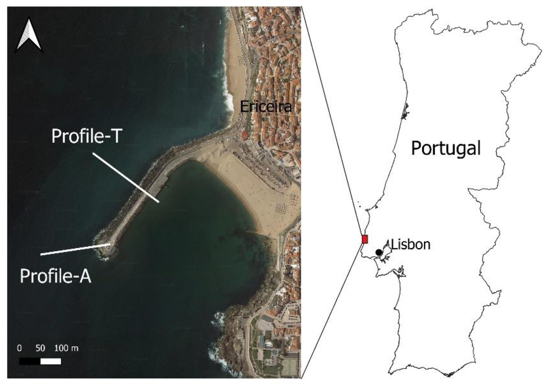
2.1. Study Site
2.2. SWASH Model Setup
2.3. Model Calibration
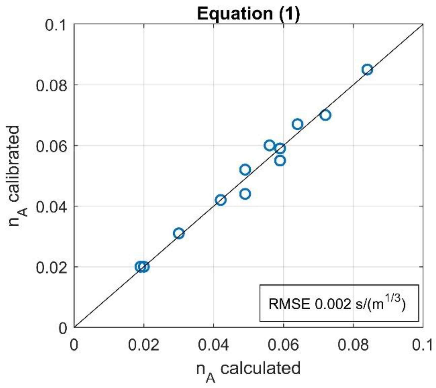
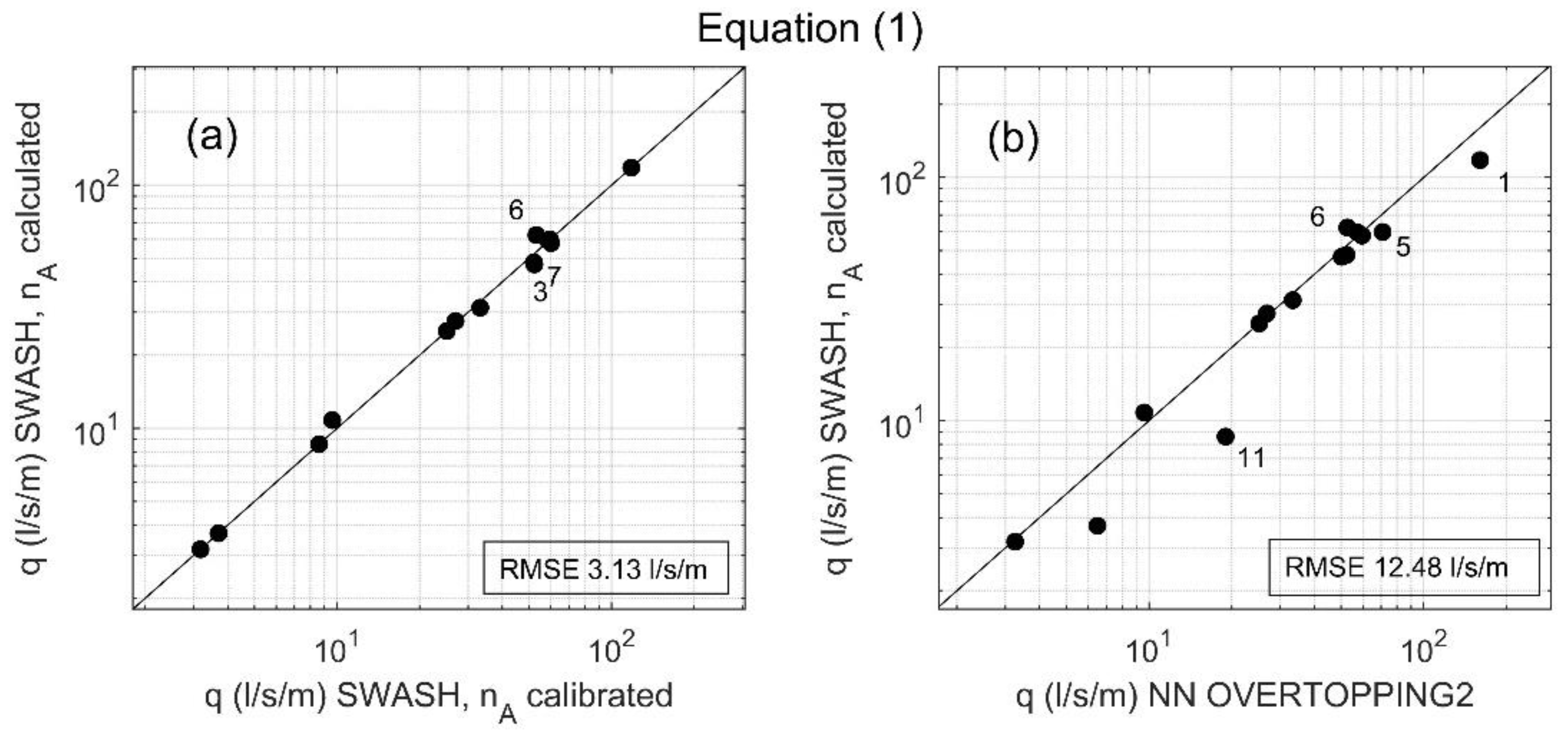
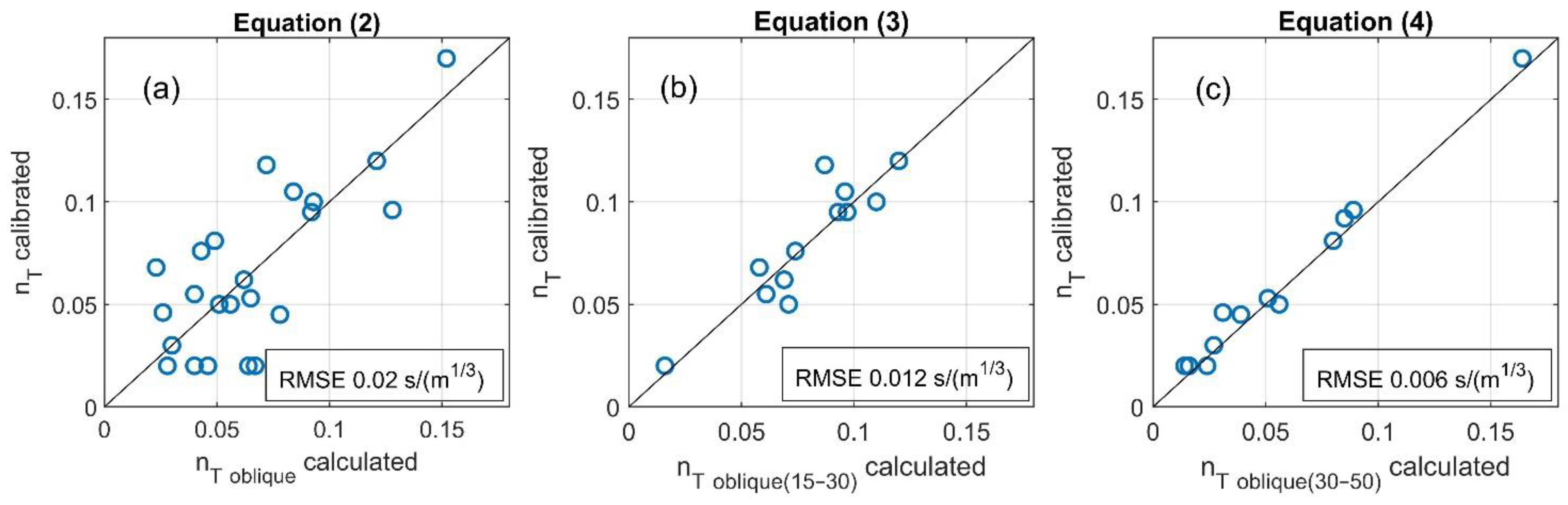
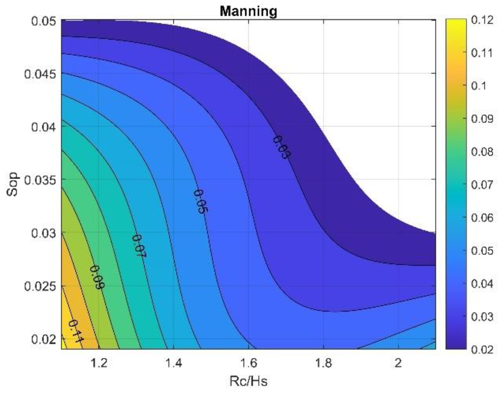
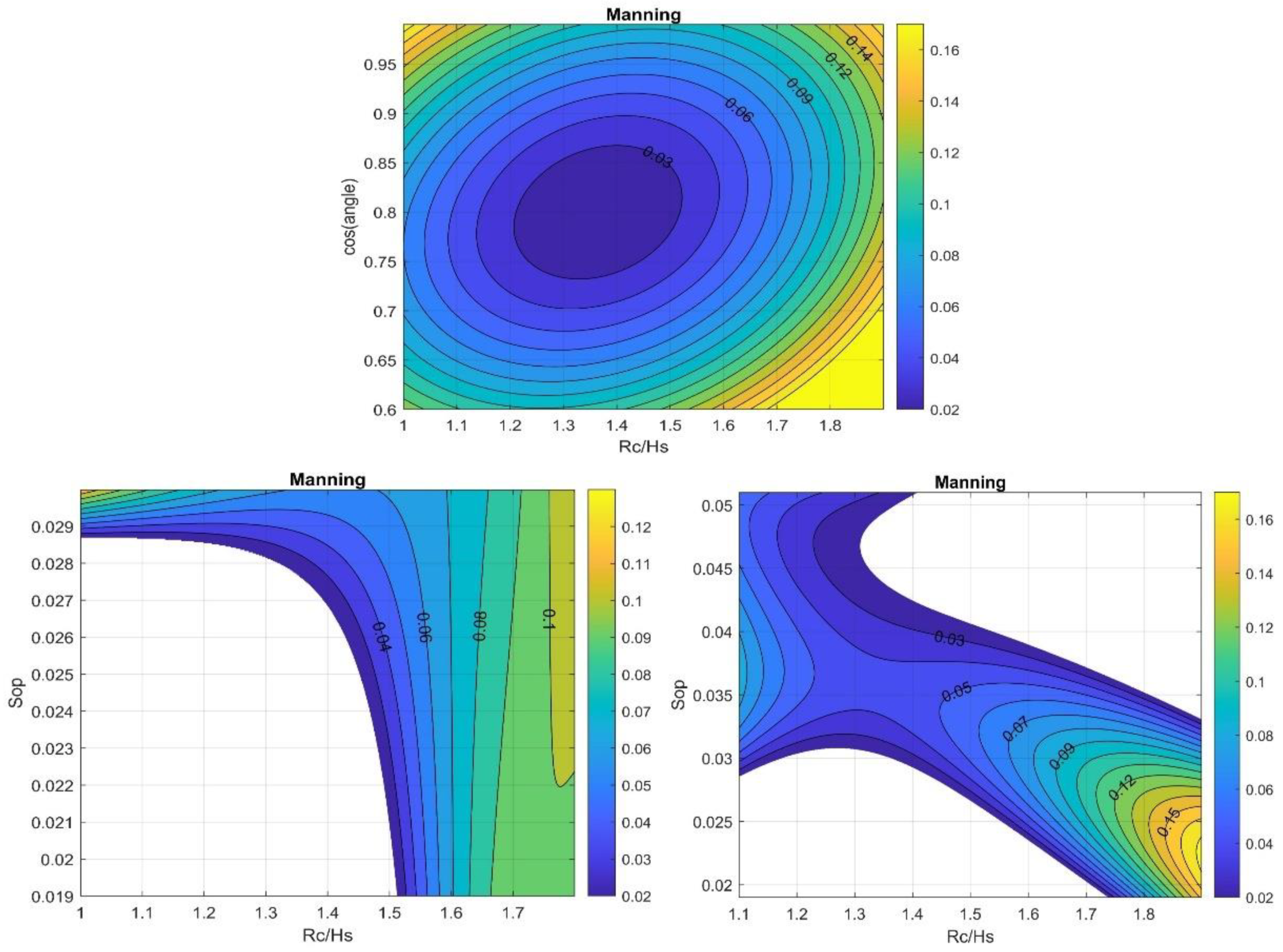
2.4. Manning Coefficient Expression Development and Validation
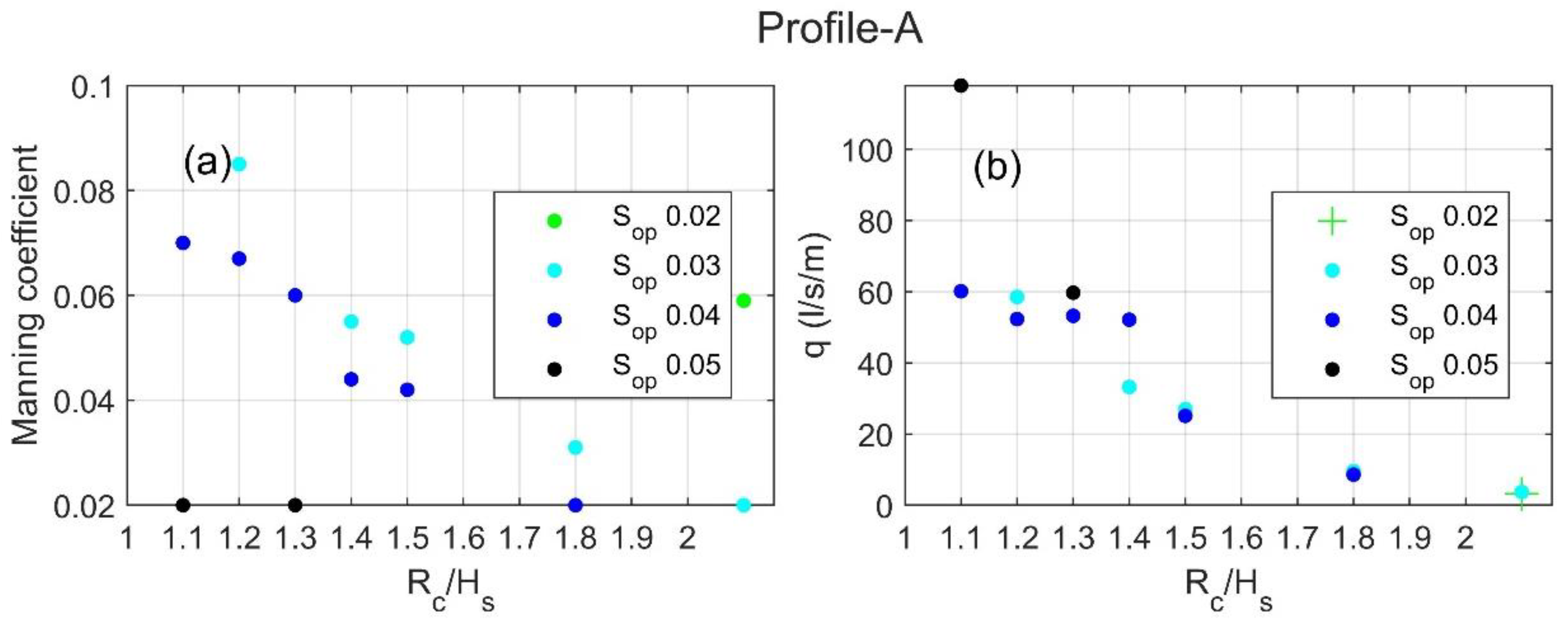
- Equation (1)—defining nA as a function of Rc/Hs and Sop, where nA is the Manning coefficient of an armour layer of antifer cubes. This equation does not account for wave obliquity and can only be applied under normal wave attack conditions, i.e., incident angles lower than 15°.
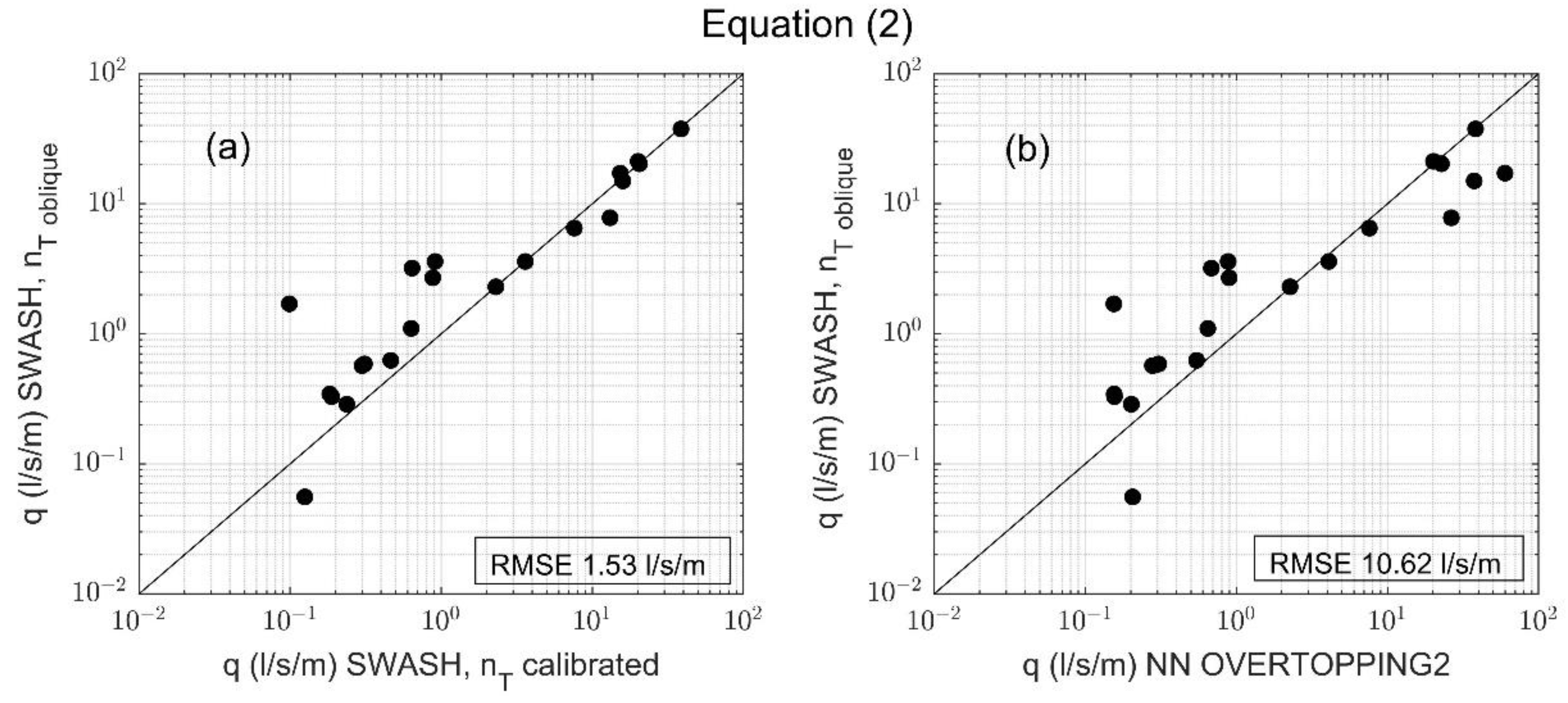
- Equation (2)—defining nT,oblique as a function of Rc/Hs and cos(β), where nT,oblique is the Manning coefficient for a tetrapod armour layer. This equation accounts for obliquity and is only applicable to oblique wave attack with incident angles greater than 15°. For that, the 24 cases were considered.
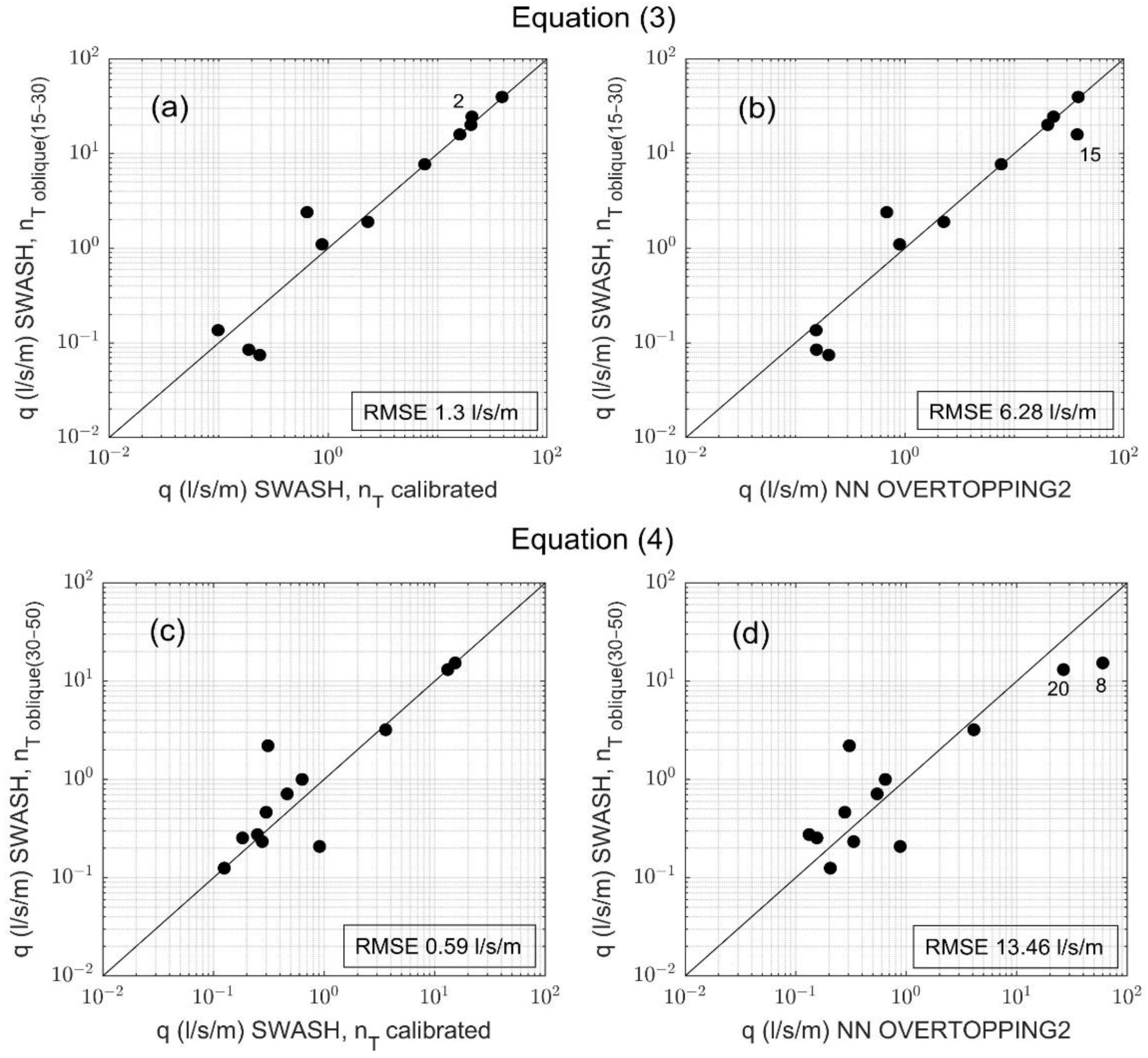
- As an alternative to Equation (2), the following Equations can be used, depending on the incident wave angle:
- Equation (3)—defining nT oblique(15–30) as a function of Rc/Hs and Sop, where nT oblique(15–30) is the Manning coefficient for a tetrapod armour layer for wave attack between 15° and 30°, based on the data from wave climate 1.
- Equation (4)—defining nT oblique(30–50) as a function of Rc/Hs and Sop, where nT oblique(30–50) is the Manning coefficient for a tetrapod armour layer for wave attack between 30° and 50°, based on the data from wave climate 2.
3. Results
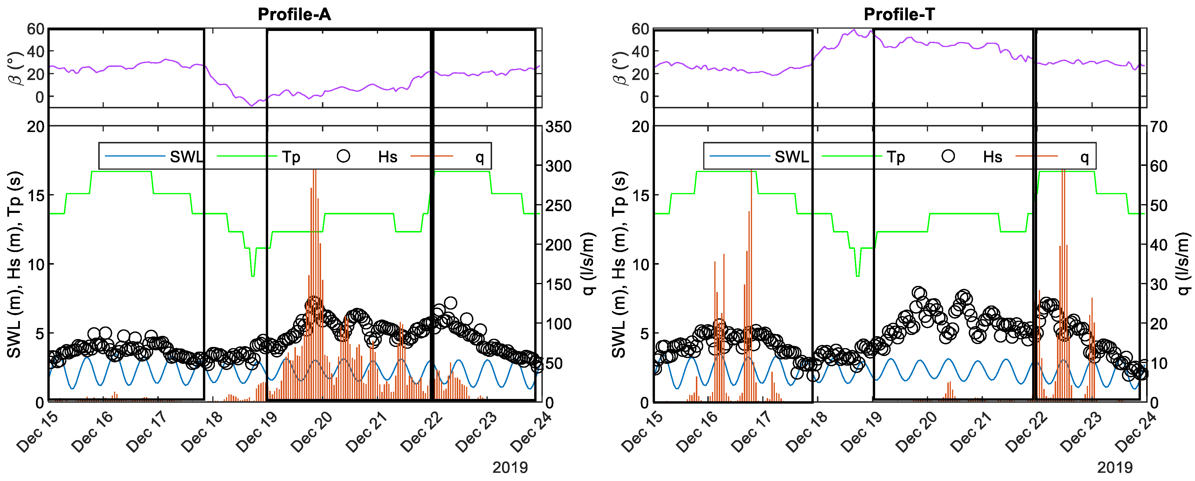
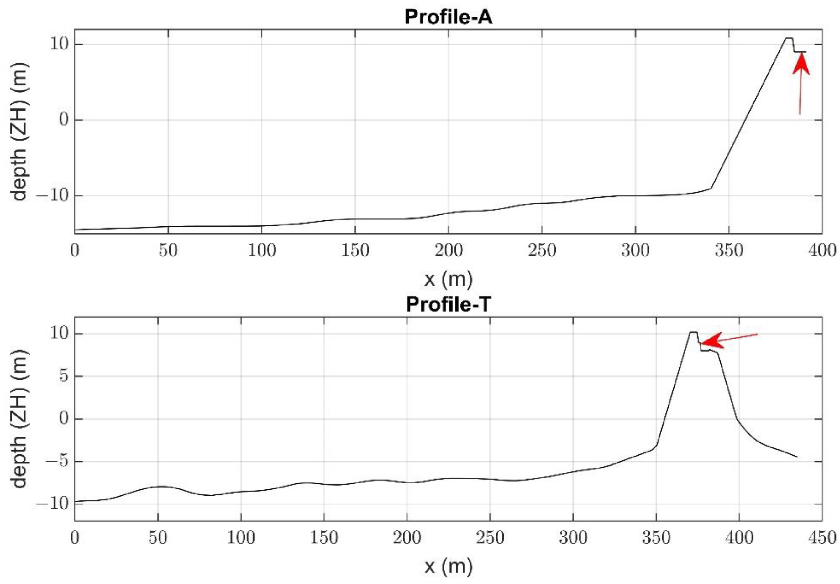
3.1. Profile-A
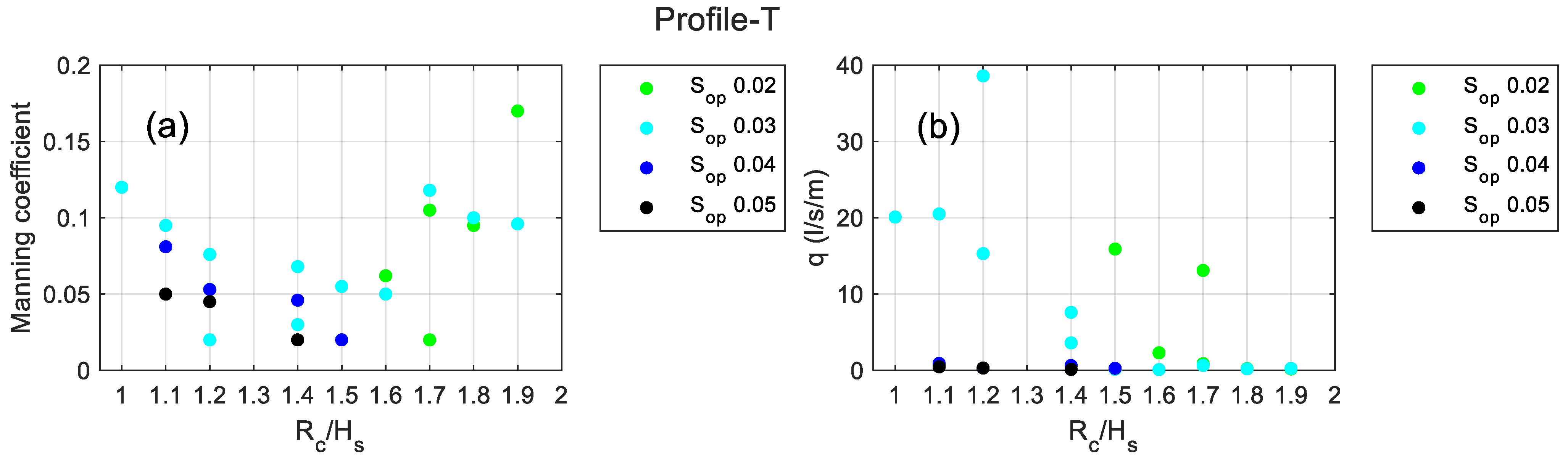
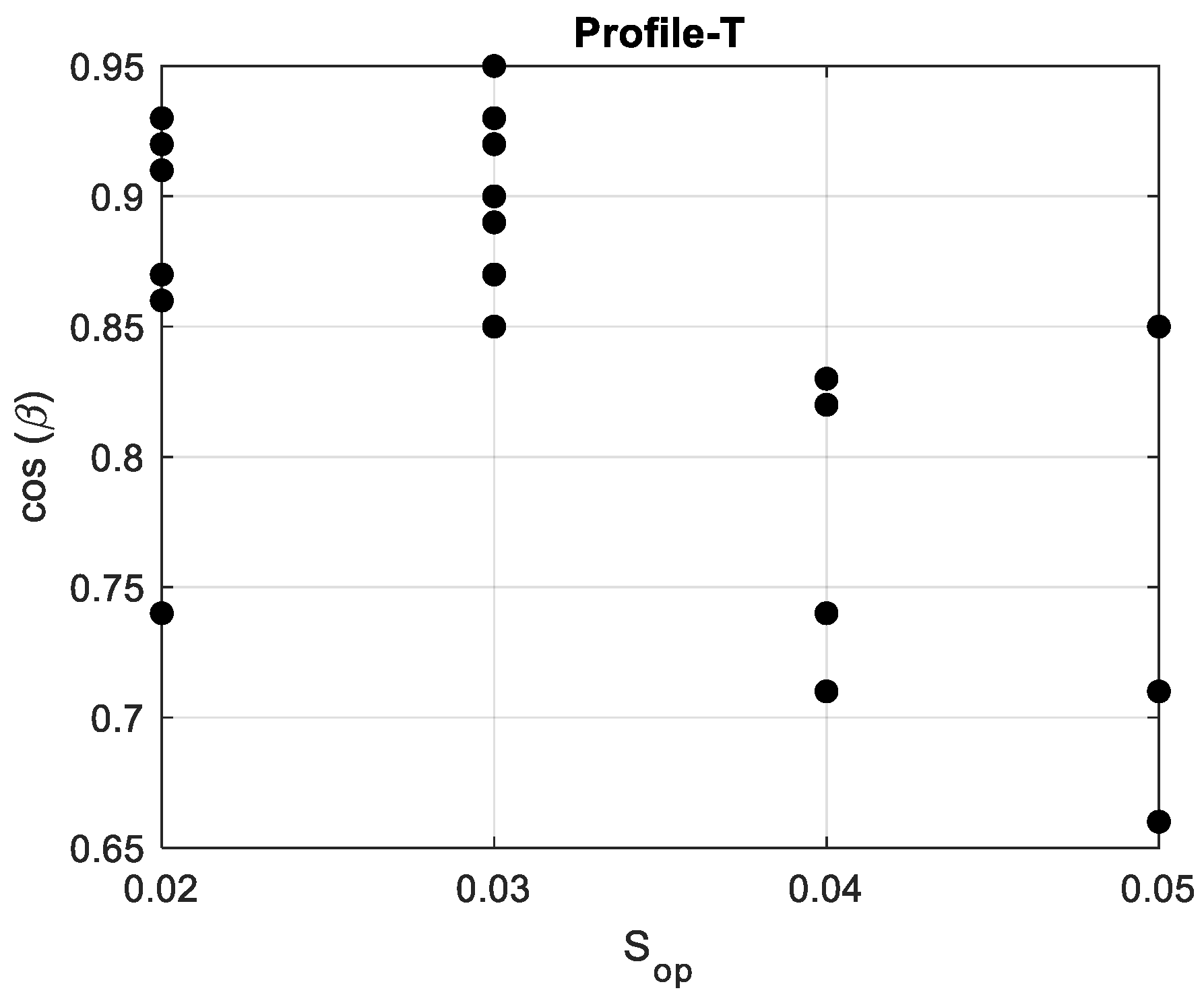
3.2. Profile-T
4. Discussion
5. Conclusions
Author Contributions
Funding
Institutional Review Board Statement
Informed Consent Statement
Acknowledgments
Conflicts of Interest
Appendix A

| Case No | q (l/s/m) NN_OVERTOPPING2 | q (l/s/m) SWASH | Manning Coefficient Calibrated (s/(m1/3)) |
|---|---|---|---|
| 1 | 160.42 | 117.91 | 0.02 |
| 2 | 59.64 | 60.14 | 0.07 |
| 3 | 50.33 | 52.34 | 0.07 |
| 4 | 57.42 | 58.50 | 0.08 |
| 5 | 70.88 | 59.72 | 0.02 |
| 6 | 52.72 | 53.20 | 0.06 |
| 7 | 52.37 | 52.11 | 0.04 |
| 8 | 33.38 | 33.24 | 0.06 |
| 9 | 25.19 | 25.14 | 0.04 |
| 10 | 26.85 | 27.02 | 0.05 |
| 11 | 19.01 | 8.60 | 0.02 |
| 12 | 9.61 | 9.62 | 0.03 |
| 13 | 6.49 | 3.74 | 0.02 |
| 14 | 3.26 | 3.18 | 0.06 |
| Case No | q (l/s/m) NN_OVERTOPPING2 | q (l/s/m) SWASH | Manning Coefficient Calibrated (s/(m1/3)) |
|---|---|---|---|
| 1 | 20.14 | 20.14 | 0.12 |
| 2 | 22.74 | 20.52 | 0.10 |
| 3 | 0.54 | 0.46 | 0.05 |
| 4 | 0.88 | 0.91 | 0.08 |
| 5 | 0.31 | 0.31 | 0.05 |
| 6 | 0.28 | 0.30 | 0.05 |
| 7 | 38.26 | 38.64 | 0.08 |
| 8 | 59.93 | 15.33 | 0.02 |
| 9 | 0.21 | 0.13 | 0.02 |
| 10 | 0.65 | 0.63 | 0.05 |
| 11 | 7.58 | 7.60 | 0.07 |
| 12 | 4.09 | 3.60 | 0.03 |
| 13 | 0.33 | 0.28 | 0.02 |
| 14 | 0.17 | 0.14 | 0.06 |
| 15 | 37.48 | 15.94 | 0.02 |
| 16 | 0.15 | 0.10 | 0.05 |
| 17 | 2.26 | 2.34 | 0.06 |
| 18 | 0.68 | 0.64 | 0.12 |
| 19 | 0.90 | 0.88 | 0.11 |
| 20 | 26.44 | 13.14 | 0.02 |
| 21 | 0.16 | 0.19 | 0.10 |
| 22 | 0.20 | 0.22 | 0.10 |
| 23 | 0.13 | 0.25 | 0.10 |
| 24 | 0.16 | 0.18 | 0.17 |
Appendix B


Appendix C


References
- Tavares, A.O.; Barros, J.L.; Freire, P.; Santos, P.P.; Perdiz, L.; Fortunato, A.B. A Coastal Flooding Database from 1980 to 2018 for the Continental Portuguese Coastal Zone. Appl. Geogr. 2021, 135, 102534. [Google Scholar] [CrossRef]
- Fortes, C.; Reis, M.T.; Poseiro, P.; Capitão, R.; Santos, J.; Pinheiro, L.; Craveiro, J.; Rodrigues, A.; Sabino, A.; Ferreira Silva, S.; et al. HIDRALERTA Project—A Flood Forecast and Alert System in Coastal and Port Areas. In Proceedings of the IWA – World Water Congress & Exhibition, Lisbon, Portugal, 21–26 September, 2014. [Google Scholar] [CrossRef]
- Pillai, K.; Etemad-Shahidi, A.; Lemckert, C. Wave Overtopping at Berm Breakwaters: Review and Sensitivity Analysis of Prediction Models. Coast. Eng. 2017, 120, 1–21. [Google Scholar] [CrossRef]
- Lavell, A.; Oppenheimer, M.; Diop, C.; Hess, J.; Lempert, R.; Li, J.; Muir-Wood, R.; Myeong, S.; Moser, S.; Takeuchi, K.; et al. Climate Change: New Dimensions in Disaster Risk, Exposure, Vulnerability, and Resilience. In Managing the Risks of Extreme Events and Disasters to Advance Climate Change Adaptation; Field, C.B., Barros, V., Stocker, T.F., Dahe, Q., Eds.; Cambridge University Press: Cambridge, UK, 2012; pp. 25–64. [Google Scholar] [CrossRef]
- van Dongeren, A.; Ciavola, P.; Martinez, G.; Viavattene, C.; Bogaard, T.; Ferreira, O.; Higgins, R.; McCall, R. Introduction to RISC-KIT: Resilience-Increasing Strategies for Coasts. Coast. Eng. 2018, 134, 2–9. [Google Scholar] [CrossRef] [Green Version]
- Gracia, V.; García-León, M.; Sánchez-Arcilla, A.; Gault, J.; Oller, P.; Fernández, J.; Sairouní, A.; Cristofori, E.; Toldrà, R. A new generation of early warning systems for coastal risk. the icoast project. Coast. Eng. Proc. 2014, 1, 1–8. [Google Scholar] [CrossRef] [Green Version]
- Poseiro, P. Forecast and Early Warning System for Wave Overtopping and Flooding in Coastal and Harbour Areas: Development of a Model and Risk Assessment; IST-UNL: Lisbon, Portugal, 2019. [Google Scholar]
- Fortes, C.J.E.M.; Reis, M.T.; Pinheiro, L.; Poseiro, P.; Serrazina, V.; Mendonça, A.; Smithers, N.; Santos, M.I.; Barateiro, J.; Azevedo, E.B.; et al. The HIDRALERTA System: Application to the Ports of Madalena Do Pico and S. Roque Do Pico, Azores. Aquat. Ecosyst. Health Manag. 2020, 23, 398–406. [Google Scholar] [CrossRef]
- Pinheiro, L.; Fortes, C.J.E.M.; Reis, M.T.; Santos, J.; Soares, C.G. Risk Forecast System for Moored Ships. Vicce Virtual Int. Conf. Coast. Eng. 2020, 36, 37. [Google Scholar] [CrossRef]
- Santos, M.I.; Pinheiro, L.; Fortes, J.C.E.M.; Reis, M.T.; Serrazina, V.; Azevedo, E.B.; Reis, F.V.; Salvador, M. Simulation of Hurricane Lorenzo at the Port of Madalena Do Pico, Azores, by Using the HIDRALERTA System. In Proceedings of the MARTECH 5th International Conference on Maritime Technology and Engineering, Lisbon, Portugal, 16–19 November 2020. [Google Scholar]
- Zózimo, A.C.; Ferreira, A.M.; Pinheiro, L.; Fortes, C.J.E.; Baliko, M. Implementação Do Sistema HIDRALERTA Para a Zona Costeira Da Costa Da Caparica. In Proceedings of the X Congresso sobre Planeamento e Gestão das Zonas Costeiras dos Países de Expressão Portuguesa, Rio de Janeiro, Brazil, 6–10 December 2021. [Google Scholar]
- Coeveld, E.M.; Van Gent, M.R.A.; Pozueta, B. Neural Network Manual for NN_Overtopping Program; Technical Report, TU Delft: Delft, The Netherlands, 2005. [Google Scholar]
- Fortes, C.J.E. Transformações Não-Lineares de Ondas Marítimas Em Zonas Portuárias. Análise Pelo Método Dos Elementos Finitos. Ph.D. Thesis, Laboratorio Nacional de Engenharia Civil, Lisboa, Portugal, 2002. [Google Scholar]
- Flater, D. Xtide. Available online: https://flaterco.com/xtide (accessed on 15 December 2021).
- Tonelli, M.; Petti, M. Numerical Simulation of Wave Overtopping at Coastal Dikes and Low-Crested Structures by Means of a Shock-Capturing Boussinesq Model. Coast. Eng. 2013, 79, 75–88. [Google Scholar] [CrossRef]
- EurOtop. Manual on Wave Overtopping of Sea Defences and Related Structures. An Overtopping Manual Largely Based on European Research, but for Worldwide Application.; Van der Meer, J.W., Allsop, N.W.H., Bruce, T., De Rouck, J., Kortenhaus, A., Pullen, T., Schüttrumpf, H., Troch, P., Zanuttigh, B., Eds. EurOtop. 2018. Available online: http://www.overtopping-manual.com (accessed on 15 December 2021).
- Suzuki, T.; Altomare, C.; Veale, W.; Verwaest, T.; Trouw, K.; Troch, P.; Zijlema, M. Efficient and Robust Wave Overtopping Estimation for Impermeable Coastal Structures in Shallow Foreshores Using SWASH. Coast. Eng. 2017, 122, 108–123. [Google Scholar] [CrossRef]
- Zijlema, M.; Stelling, G.; Smit, P. SWASH: An Operational Public Domain Code for Simulating Wave Fields and Rapidly Varied Flows in Coastal Waters. Coast. Eng. 2011, 58, 992–1012. [Google Scholar] [CrossRef]
- Suzuki, T.; Verwaest, T.; Veale, W.; Trouw, K.; Zijlema, M. A numerical study on the effect of beach nourishment on wave overtopping in shallow foreshores. Coast. Eng. Proc. 2012, 1. [Google Scholar] [CrossRef] [Green Version]
- Suzuki, T.; Altomare, C.; Verwaest, T.; Trouw, K.; Zijlema, M. Two-dimensional wave overtopping calculation over a dike in shallow foreshore by swash. Coast. Eng. Proc. 2014, 1, Structures.3. [Google Scholar] [CrossRef] [Green Version]
- Zhang, N.; Zhang, Q.; Wang, K.-H.; Zou, G.; Jiang, X.; Yang, A.; Li, Y. Numerical Simulation of Wave Overtopping on Breakwater with an Armor Layer of Accropode Using SWASH Model. Water 2020, 12, 386. [Google Scholar] [CrossRef] [Green Version]
- Celli, D.; Pasquali, D.; De Girolamo, P.; Di Risio, M. Effects of Submerged Berms on the Stability of Conventional Rubble Mound Breakwaters. Coast. Eng. 2018, 136, 16–25. [Google Scholar] [CrossRef]
- Liang, B.; Wu, G.; Liu, F.; Fan, H.; Li, H. Numerical Study of Wave Transmission over Double Submerged Breakwaters Using Non-Hydrostatic Wave Model. Oceanologia 2015, 57, 308–317. [Google Scholar] [CrossRef] [Green Version]
- Hersbach, H.; Bell, B.; Berrisford, P.; Biavati, G.; Horányi, A.; Muñoz Sabater, J.; Nicolas, J.; Peubey, C.; Radu, R.; Rozum, I.; et al. ERA5 Hourly Data on Single Levels from 1959 to Present; Copernicus Climate Change Service (C3S) Climate Data Store (CDS): Reading, UK, 2018. [Google Scholar] [CrossRef]
- Swan Team. Swan User Manual, 40.51.; Department of Civil Engineering and Geosciences, Delft university of Technology: Delft, The Netherlands, 2006. [Google Scholar]
- Pés, V.M. Applicability and Limitations of the SWASH Model to Predict Wave Overtopping; TU Delft: Delft, The Netherlands; Universitat Politecnica de Catalunya: Barcelona, Spain, 2013. [Google Scholar]
- Salas Pérez, M. Overtopping over a Real Rubble Mound Breakwater Calculated with SWASH; Universitat Politecnica de Catalunya: Barcelona, Spain; Delft University of Technology: Delft, The Netherlands, 2014. [Google Scholar]
- TAW. Technisch Rapport Golfoploop En Golfoverslag Bij Dijken (Technical Report on Wave Run-up and Wave Overtopping at Dikes—In Dutch); Technical Advisory Committee on Flood Defence: Brussels, Belgium, 2002. [Google Scholar]
- Galland, J.C. Rubble mound breakwater stability under oblique waves: And experimental study. Coast. Eng. Proc. 1994, 1, 24. [Google Scholar] [CrossRef]
- Vanneste, D.F.A.; Altomare, C.; Suzuki, T.; Troch, P.; Verwaest, T. Comparison of numerical models for wave overtopping and impact on a sea wall. Coast. Eng. Proc. 2014, 1, 5. [Google Scholar] [CrossRef]
- Manz, A. Application of SWASH to Determine Overtopping during Storm Events in the Port of Ericeira and Its Introduction into HIDRALERTA System; Universidade do Algarve: Faro, Portugal, 2021. [Google Scholar]


| Slope | Rc (m) | Ac (m) | Gc (m) | |
|---|---|---|---|---|
| Profile-A | 1:2.0 | 9.03 | 10.85 | 5.79 |
| Profile-T | 1:1.5 | 8.98 | 10.20 | 5.28 |
| Case No | Date and Time | Rc/Hs | Sop | Hs (m) | Tp (s) | SWL (m) | Incident Wave Angle β (°) |
|---|---|---|---|---|---|---|---|
| 1 | 19 December 2019, 18:00 | 1.10 | 0.05 | 6.03 | 12.33 | 2.39 | 2.00 |
| 2 | 20 December 2019, 01:00 | 1.10 | 0.04 | 6.19 | 13.64 | 1.97 | 5.00 |
| 3 | 20 December 2019, 03:00 | 1.20 | 0.04 | 6.07 | 13.64 | 1.68 | 5.00 |
| 4 | 20 December 2019, 07:00 | 1.20 | 0.03 | 5.20 | 13.64 | 2.70 | 8.00 |
| 5 | 19 December 2019, 15:00 | 1.30 | 0.05 | 5.90 | 12.33 | 1.55 | 2.00 |
| 6 | 19 December 2019, 10:00 | 1.30 | 0.04 | 4.68 | 12.33 | 2.77 | 3.00 |
| 7 | 19 December 2019, 11:00 | 1.40 | 0.04 | 4.85 | 12.33 | 2.39 | 0.40 |
| 8 | 21 December 2019, 08:00 | 1.40 | 0.03 | 4.46 | 12.33 | 2.59 | 4.00 |
| 9 | 18 December 2019, 22:00 | 1.50 | 0.04 | 4.45 | 11.14 | 2.45 | 4.00 |
| 10 | 19 December 2019, 06:00 | 1.50 | 0.03 | 4.15 | 12.33 | 2.76 | 3.00 |
| 11 | 19 December 2019, 00:00 | 1.80 | 0.04 | 4.03 | 11.14 | 1.80 | 2.00 |
| 12 | 19 December 2019, 02:00 | 1.80 | 0.03 | 4.10 | 12.33 | 1.58 | 1.00 |
| 13 | 18 December 2019, 10:00 | 2.10 | 0.03 | 3.28 | 12.33 | 2.28 | 1.00 |
| 14 | 18 December 2019, 05:00 | 2.10 | 0.02 | 2.95 | 13.64 | 2.79 | 11.00 |
| Case No | Date and Time | Rc/Hs | Sop | Hs (m) | Tp (s) | SWL (m) | Incident Wave Angle β (°) |
|---|---|---|---|---|---|---|---|
| 1 | 16 December 2019. 05:00 | 1.00 | 0.03 | 5.57 | 16.69 | 3.50 | 23.00 |
| 2 | 16 December 2019. 06:00 | 1.10 | 0.03 | 5.23 | 16.69 | 3.41 | 23.00 |
| 3 | 20 December 2019. 06:00 | 1.10 | 0.05 | 6.02 | 13.64 | 2.35 | 45.00 |
| 4 | 20 December 2019. 20:00 | 1.10 | 0.04 | 5.83 | 13.64 | 3.06 | 42.00 |
| 5 | 19 December 2019. 18:00 | 1.20 | 0.05 | 5.43 | 12.33 | 2.39 | 49.00 |
| 6 | 21 December 2019. 07:00 | 1.20 | 0.04 | 5.64 | 13.64 | 2.21 | 45.00 |
| 7 | 16 December 2019. 17:00 | 1.20 | 0.03 | 4.81 | 16.69 | 3.21 | 21.00 |
| 8 | 22 December 2019. 12:00 | 1.20 | 0.03 | 4.84 | 16.69 | 3.03 | 32.00 |
| 9 | 21 December 2019. 14:00 | 1.40 | 0.05 | 5.10 | 12.33 | 2.06 | 32.00 |
| 10 | 21 December 2019. 13:00 | 1.40 | 0.04 | 4.70 | 12.33 | 2.49 | 34.00 |
| 11 | 17 December 2019. 04:00 | 1.40 | 0.03 | 4.27 | 15.09 | 2.92 | 18.00 |
| 12 | 22 December 2019. 22:00 | 1.40 | 0.03 | 4.53 | 16.69 | 2.53 | 30.00 |
| 13 | 21 December 2019. 20:00 | 1.50 | 0.04 | 4.51 | 13.64 | 2.14 | 35.00 |
| 14 | 15 December 2019. 22:00 | 1.50 | 0.03 | 5.02 | 16.69 | 1.25 | 27.00 |
| 15 | 16 December 2019. 07:00 | 1.50 | 0.02 | 3.96 | 16.69 | 3.06 | 25.00 |
| 16 | 15 December 2019. 14:00 | 1.60 | 0.03 | 4.11 | 15.09 | 2.35 | 27.00 |
| 17 | 16 December 2019. 15:00 | 1.60 | 0.02 | 3.93 | 16.69 | 2.54 | 23.00 |
| 18 | 15 December 2019. 15:00 | 1.70 | 0.03 | 3.66 | 15.09 | 2.80 | 26.00 |
| 19 | 17 December 2019. 08:00 | 1.70 | 0.02 | 3.56 | 15.09 | 2.83 | 21.00 |
| 20 | 23 December 2019. 00:00 | 1.70 | 0.02 | 3.53 | 16.69 | 3.06 | 31.00 |
| 21 | 15 December 2019. 03:00 | 1.80 | 0.03 | 3.28 | 13.64 | 3.15 | 29.00 |
| 22 | 15 December 2019. 06:00 | 1.80 | 0.02 | 3.24 | 13.64 | 3.07 | 30.00 |
| 23 | 23 December 2019. 03:00 | 1.90 | 0.03 | 3.63 | 15.09 | 2.14 | 30.00 |
| 24 | 18 December 2019. 06:00 | 1.90 | 0.02 | 3.07 | 13.64 | 3.08 | 42.00 |
Publisher’s Note: MDPI stays neutral with regard to jurisdictional claims in published maps and institutional affiliations. |
© 2022 by the authors. Licensee MDPI, Basel, Switzerland. This article is an open access article distributed under the terms and conditions of the Creative Commons Attribution (CC BY) license (https://creativecommons.org/licenses/by/4.0/).
Share and Cite
Manz, A.; Zózimo, A.C.; Garzon, J.L. Application of SWASH to Compute Wave Overtopping in Ericeira Harbour for Operational Purposes. J. Mar. Sci. Eng. 2022, 10, 1881. https://doi.org/10.3390/jmse10121881
Manz A, Zózimo AC, Garzon JL. Application of SWASH to Compute Wave Overtopping in Ericeira Harbour for Operational Purposes. Journal of Marine Science and Engineering. 2022; 10(12):1881. https://doi.org/10.3390/jmse10121881
Chicago/Turabian StyleManz, Anika, Ana Catarina Zózimo, and Juan L. Garzon. 2022. "Application of SWASH to Compute Wave Overtopping in Ericeira Harbour for Operational Purposes" Journal of Marine Science and Engineering 10, no. 12: 1881. https://doi.org/10.3390/jmse10121881