Article

Mapping Dependence between Extreme Skew-Surge, Rainfall, and River-Flow

1
National Institute of Water and Atmospheric Research, P.O. Box 11115, Hamilton 3251, New Zealand
2
Department of Infrastructure, University of Melbourne, Level 6, Melbourne Connect, 700 Swanston St., Carlton, VIC 3053, Australia
*
Author to whom correspondence should be addressed.
J. Mar. Sci. Eng. 2022, 10(12), 1818; https://doi.org/10.3390/jmse10121818
Submission received: 26 September 2022 / Revised: 8 November 2022 / Accepted: 21 November 2022 / Published: 25 November 2022
(This article belongs to the Special Issue Coastal Flooding: Causes, Impacts and Mitigation)

Abstract

:
Flooding in coastal areas is a major global hazard, made worse during compound flood events, which occur when multiple flood-drivers, such as tide, sea surge, and fluvial and pluvial flooding, coincide. We use 12 sea-level, 2065 rainfall, and 81 river-flow records to assess the dependence of (1) extreme skew-surge and extreme rainfall (pluvial/surface runoff) and (2) extreme skew-surge and extreme river-flow (fluvial discharge) in New Zealand. We found that (1) skew-surge and rainfall and (2) skew-surge and river-flow are significantly, but not strongly, correlated in NZ. When spatially averaged to within 30 km of sea-level gauge location, the correlation was generally significant and positive, but weak with Kendall’s rank correlation coefficient τ < 0.3. We identify the weather types driving regional patterns of dependence. Trough weather types were the dominant driver of individual and coincident extreme events. Blocking weather types were associated with the highest extreme skew-surge and rainfall events along the northeast coast of the North Island and, consequently, were associated with a high proportion of coincident skew-surge/rainfall and skew-surge/river-flow events there. These findings have important implications for flood management, emergency response, and the insurance sector because impacts and losses may be correlated in space. Our findings add to a growing understanding of compound flooding worldwide for different geographical and meteorological settings. The positive dependence observed suggests that more attention to compound event probabilities is warranted when undertaking localized coastal-flood modelling.

1. Introduction

Flooding in coastal areas is a major global hazard with historical events killing 100,000s of people and causing billions of dollars of damages, e.g., [1,2,3]. Millions of people are exposed to a 1 in 100-year flood from the sea, e.g., [4,5,6,7]. In New Zealand, this includes 1.5% of the population [8] and billions of dollars of critical infrastructure [8].
Flooding in coastal areas can result from combinations of high coastal water levels (combinations of tides, surge, and waves) and freshwater runoff (high rainfall or river-flow). Events where both coastal and freshwater processes combine are known as compound flooding events and can result in greater flood impact than either coastal or freshwater flooding alone [9,10,11,12,13]. There is increasing recognition of the importance to better understand compound events that lead to extreme impacts, e.g., [14,15,16].
Research has quantified the dependence between coastal and freshwater flood-hazard drivers at national [11,17,18,19,20,21] and international [22] scales. Most studies quantifying dependence have focused on two (bivariate) variables: (1) sea surge and (2) either (a) rainfall [18,19,20] or (b) freshwater runoff [9,11,21,22]. Nasr et al. [17] quantified the dependence between several pairs of hazard drivers: storm surge, waves, fluvial (excessive river discharge), and pluvial (surface runoff). Place-based studies have been used to quantify impacts [9,10,11,12,13,21]—these studies show that there is typically a seaward zone of mainly coastal influence, an inland zone of freshwater-only influence, and a complex intermediary zone of compound influence which depends on the geographical setting and the nature of the compound event (e.g., relative size of coastal and freshwater drivers). Some studies have related the compound events to meteorological conditions [18,19].
Here, we investigate the dependence of meteorologically-driven coastal-hazard drivers as a first step toward understanding compound coastal flooding events in New Zealand. We use available sea-level, rainfall, and river-flow measurements to assess the dependence of (1) extreme skew-surge and extreme rainfall (pluvial/surface runoff) and (2) extreme skew-surge and extreme river-flow (fluvial discharge) in New Zealand. We identify the weather types driving regional patterns of dependence. This is the first comprehensive analysis of dependence between oceanographic, fluvial, and pluvial flooding drivers in New Zealand and contributes to a growing understanding of compound flooding worldwide for different geographical and meteorological settings. During this process, we identify regional patterns in dependence which could lead to compound flood events, and the weather types that cause them, which could inform early-warning tools via meteorological forecasts. Knowledge of regional patterns of flood-hazard dependence can show where more detailed compound flood impact modelling should be undertaken.

2. Methods

2.1. Dependence Measure

Following Wahl et al. [18], we used Kendall’s rank correlation coefficient τ [23] to reliably measure dependence between the two variables. Whereas Pearson’s correlation coefficient captures linear, normally-distributed relationships between variables, Kendall’s τ measures the monotonic relationship, is non-parametric, and is a statistic of dependence between two variables. Kendall’s τ is based on counting the number of (i,j) pairs, for i < j, that are concordant—that is, for which xixj have the same sign (Equation (1)). Let (x1, y1),…, (xn, yn) be a set of observations of the joint random variables X and Y, such that all the values of xi and y1 are unique. Any pair of observations (xi, yi) and (xj, yj), where i < j are said to be concordant if the sort order of (xi, xj) and (yi, yj) agrees: that is, if either both xi > xj and yi > yj holds or both xi < xj and yi < yj; otherwise they are said to be discordant. The statistical significance of the correlation was determined using a p-value of ≤0.05.
Equation (1). Kendall’s rank correlation coefficient: where x and y represent the two variables whose correlation is being compared and n = the number of observations:
τ = 2 n ( n 1 ) i < j s i g n ( x i x j )   s i g n ( y i y j )

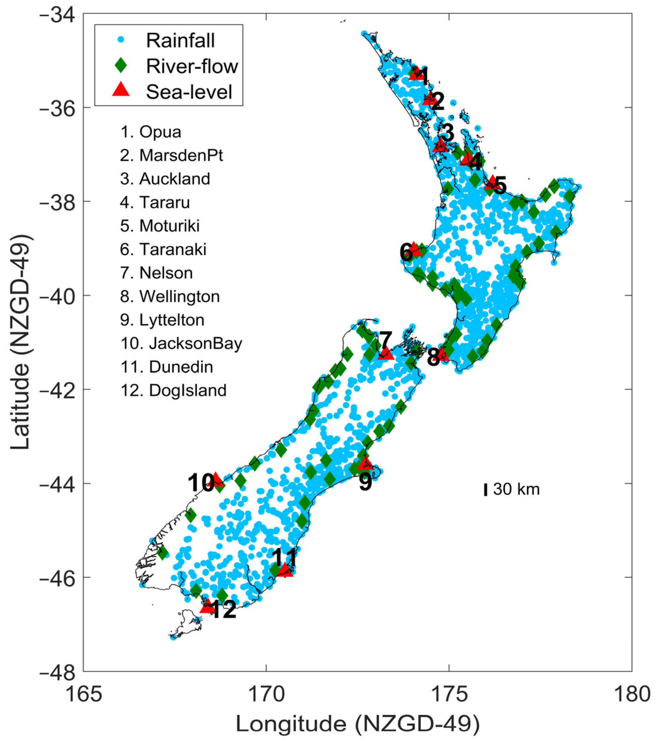
2.2. Data selection and Processing

Kendall’s τ was calculated using overlapping timeseries of daily maximum skew-surge, daily cumulative rainfall, and daily maximum river flow.
To obtain skew-surge, we analyzed a subset of the same 30 hourly sea-level records analyzed by Stephens, et al. [24]. Skew-surge was calculated as the absolute difference between the maximum recorded sea level and the predicted maximum astronomical tidal level for each ~12.5-h tidal cycle [25,26]—every high tide has an associated skew-surge. Skew-surge is a relevant metric of surge in tidally dominant locations such as NZ, e.g., [27], because the extreme sea level and resulting flooding exposure usually occurs for a few hours around the high tide [24,27]. The daily maximum skew-surge was extracted from the skew-surge records.
Tsunamis affect sea-levels, but are not meteorologically derived. Coincident events were removed from the records on the following days because of tsunami: 28 February 2010 and 29 September 2009. Tsunami events were observed in the sea-level records on other dates, but did not coincide with extreme rainfall or river flow.
Sufficient overlap in surge/rainfall or surge/river-flow records is needed to determine statistically significant correlations. Only record pairs that satisfied skew-surge and rainfall/river-flow ≥ 20-years overlap at ≥75% annual completion were included in the analysis. The sole exception was the inclusion of the Jackson Bay sea-level record (Site 18, Figure 1), where 15-years overlap was accepted because it filled a geographical gap on the South Island west coast. This resulted in 12 sea-level, 2065 rainfall, and 81 river-flow records being used (Figure 1).
Kendall’s τ and p-value were calculated for four cases of dependence, as described in Table 1; for example, skew-surge and rainfall with rainfall conditional on extreme skew-surge (SS/R|SS)—meaning that extreme skew-surge events are identified and for each extreme skew-surge a search is conducted to find extreme rainfall events within a time window of the skew-surge event.
This requires a definition of “extreme” skew-surge, rainfall, and river-flow in order to select the significantly large events for analysis. One option is to apply a block maxima approach such as using the annual maximum, but because this only uses the single highest value in a year, this eliminates genuinely large events when more than one per year occurs [28]. Therefore, we applied a more inclusive peaks-over-threshold (POT) approach [28]. A generalized Pareto distribution (GPD) is a statistically robust method for modelling the frequency and magnitude of extreme values using POT data [28]. An appropriate threshold to fit the GPD is the lowest threshold where the shape and scale parameters of the GPD are approximately constant within 95% confidence intervals of the GPD fit. We determined these thresholds for each skew-surge, rainfall, and river-flow record. Values above these thresholds were used in the analysis, with the over-threshold maxima being separated by a minimum of 3 days, since separate meteorological systems generally pass over NZ within 4–7 days of each other.
For the analysis of dependence, paired timeseries were created as follows (e.g., Figure 2):
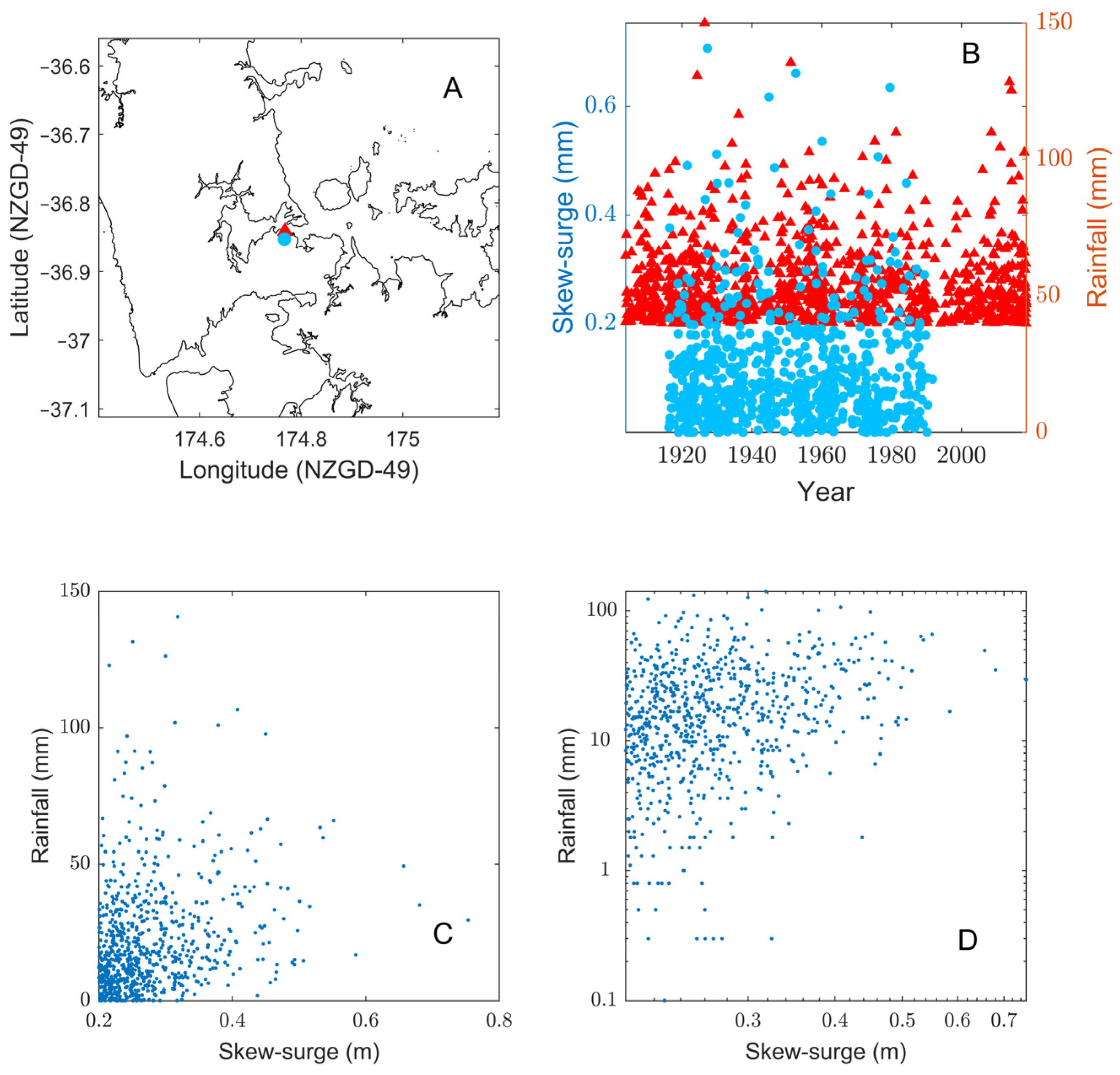
  • For each skew-surge, rainfall, and river-flow record, identify all daily maxima ≥thresholds.
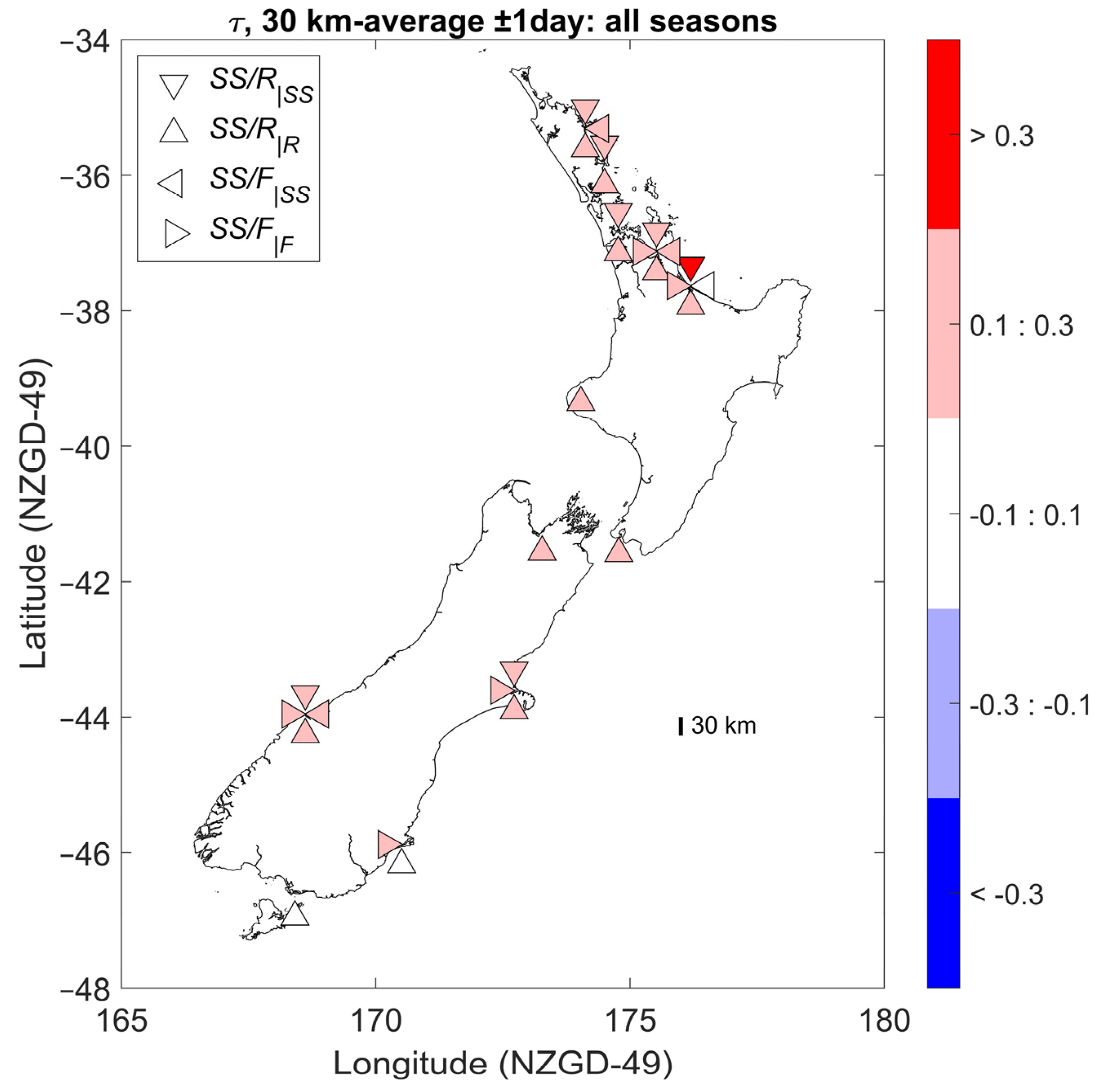
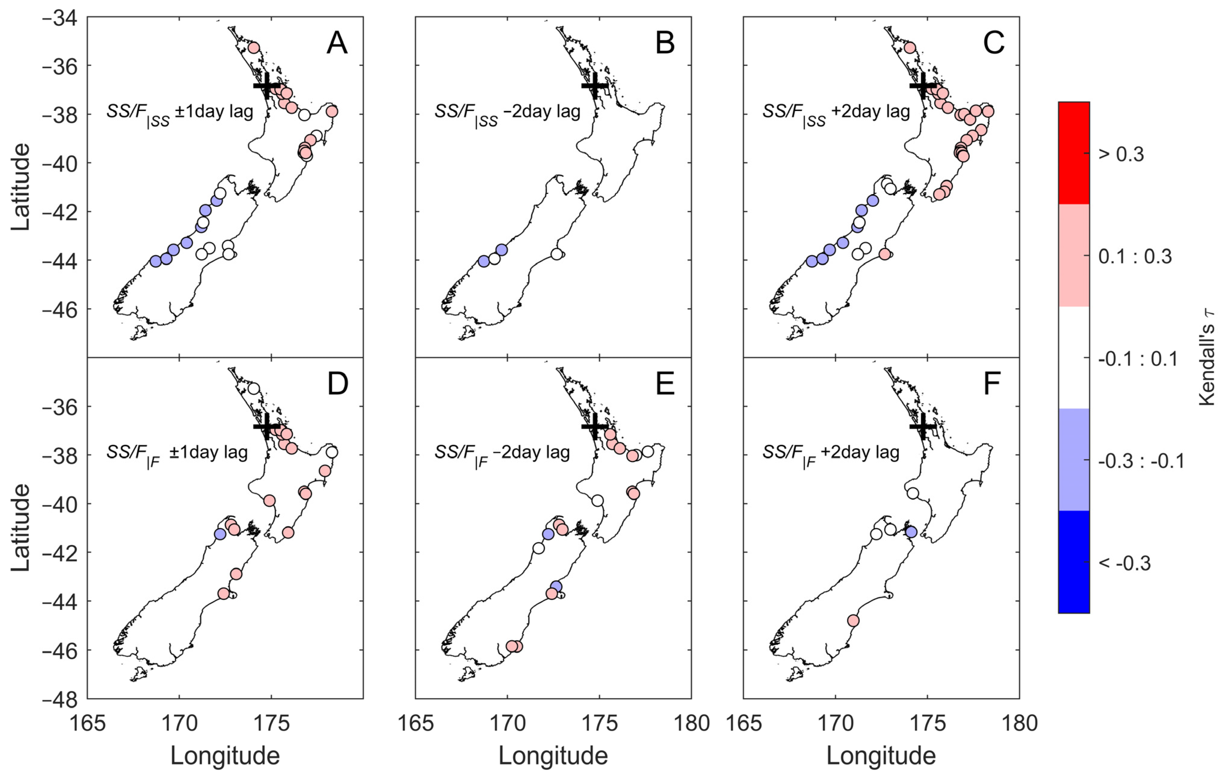
  • Then, using each (skew-surge, rainfall, and river-flow) variable in turn as the conditional variable, we extract time-series of the other variable using time-lags from −5 to +5 days, and also (maximum within) ±1-day. For example, for SS/R|SS, we identify POT values of skew-surge, and then select corresponding rainfall with time lags of −5, −4, −3, −2, −1, 0, +1, +2, +3, +4, +5, and (maximum within) ±1 days.
  • For each lagged timeseries, we then calculate and record τ and p-value.
Regional patterns of dependence were assessed using spatial averages of Kendall’s rank correlation coefficient within 30 km of sea-level gauge for SS/R and SS/F using a ± 1-day window. We trialed larger averaging radii of up to 100 km (not shown) and found that the dependence reduced as the sampling radius increased. A 100 km radius was used at Jackson Bay due to the low rainfall and river-flow sampling density near the Jackson Bay sea-level recorder. The spatial averaging was performed by averaging the τ already calculated between individual gauge timeseries pairs—not by combining rainfall or river-flow records before calculating τ. Only τ significant at p-value ≤ 0.05 were used for the spatial averages.
We used the Kidson [29] weather regimes (Figure 3) to investigate the weather regimes driving spatial patterns of dependence between skew-surge, rainfall, and river-flow. Kidson [29] identified 12 “typical” daily weather pattern types for the New Zealand region. Each of these patterns looks realistic, in the sense that they might be recognized in daily weather maps. Cluster analysis of the monthly frequencies of these patterns led to the definition of three weather “regimes”, characterized by: (i) frequent low-pressure troughs crossing the country, (ii) high-pressure systems to the north with strong zonal flow to the south of the NZ, and (iii) blocking patterns with high-pressure systems more prominent in the south (Figure 3). The Kidson [29] types and weather regimes are widely cited, having been shown to influence spatial patterns of atmospheric vapor transport [30], precipitation and temperature anomalies [31], atmospheric circulation patterns during large snowfall events [32], extreme rainfall [33], and extreme skew-surge [24], for example.
The dependence analysis was performed for the four cases described in Table 1, which provides a useful way to rank the dependence using Kendall’s rank correlation coefficient. However, ranking the variables like this (e.g., choosing extreme events for one variable and then taking the matching daily value for the other variable) does not ensure that both variables are extreme at the same time. Therefore, for the Kidson-type analysis, we identified composite events where both skew-surge and rainfall were both above their respective 95% thresholds. We used a 90% threshold for the skew-surge and river-flow analysis to capture more events, due to the lower spatial density of river-flow records relative to rainfall records. We obtained a database of daily Kidson types from Dr. James Renwick [34]. We matched each composite weather event with its Kidson type and weather regime.

3. Results

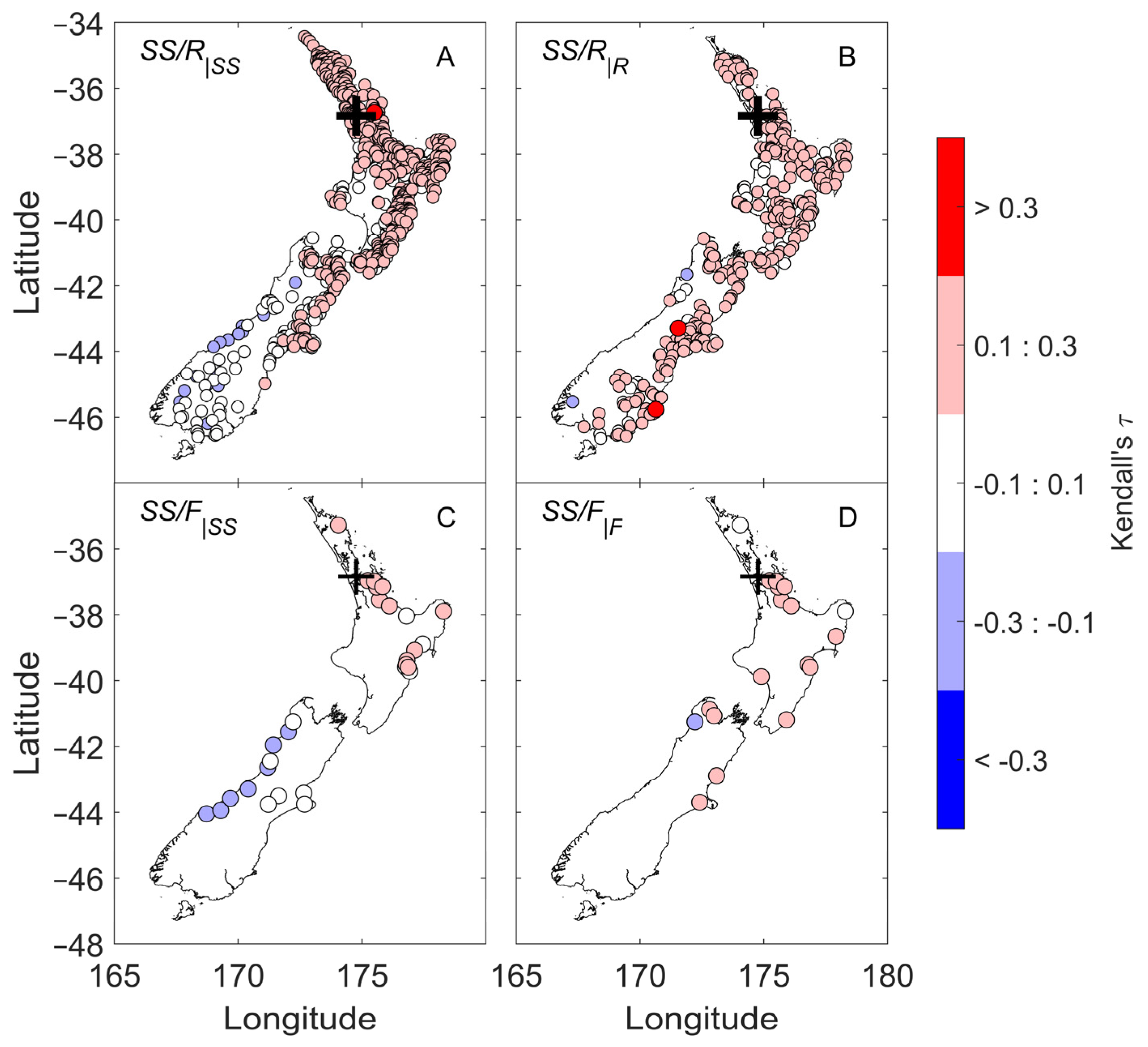
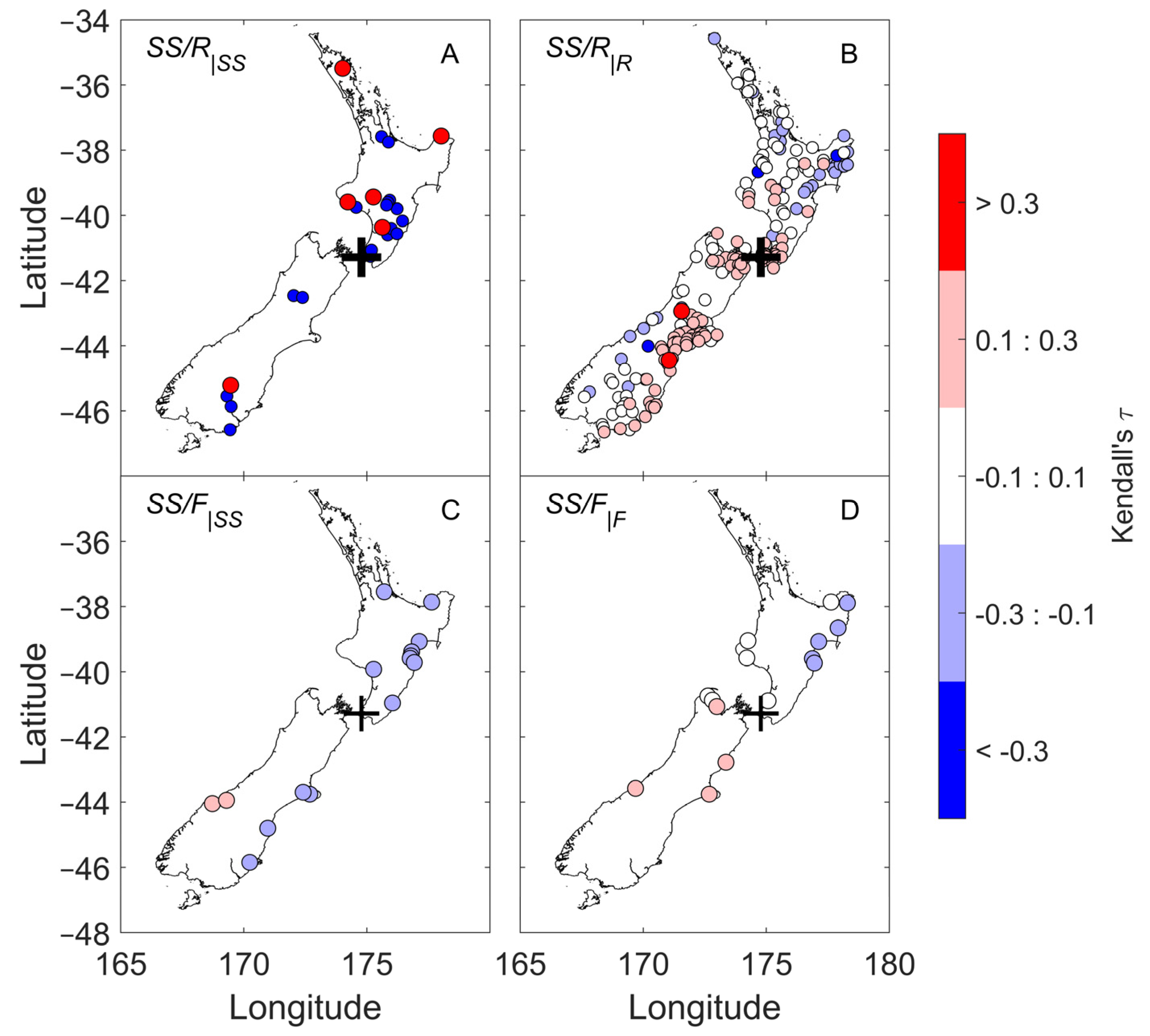
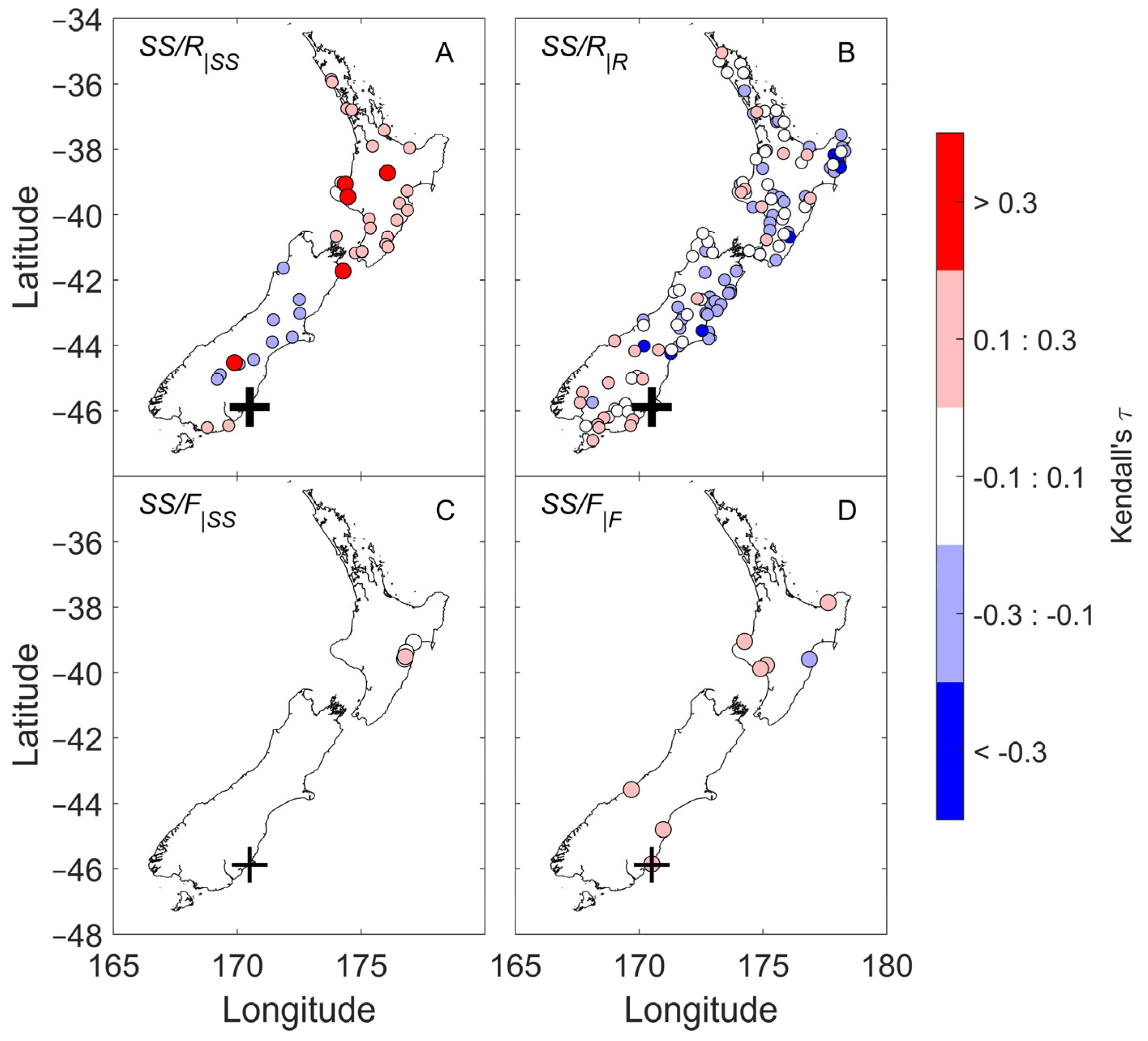
3.1. Spatial Patterns of Dependence

We found that (1) skew-surge and rainfall and (2) skew-surge and river-flow are significantly, but not strongly, correlated in NZ. The spatial average of τ within 30 km of the sea-level gauge location showed that correlations were sometimes significant (at p-value < 0.05) and were generally weakly positive (|τ| < 0.3) (Figure 4). Correlations between skew-surge and river-flow were significant at fewer sea-level record sites than for skew-surge and rainfall (Figure 4). Other than the SS/R|R case, spatially-averaged correlations appear to be insignificant in the center of New Zealand (lower North and upper South Islands) (Figure 4).
Spatial patterns in dependence were noticeable. Here, we focus on paired observations within ±1-day of an extreme event for the four longest sea-level records: Auckland (Figure 5), Wellington (Figure 6), Lyttelton (Figure 7), and Dunedin (Figure 8)—these four sites also span a large north-south range for New Zealand. It can be seen that spatial patterns of dependence are generally similar between (1) skew-surge and rainfall and (2) skew-surge and river-flow, e.g., if rainfall is positively correlated with surge near a sea-level recorder site, then river-flow also tends to be positively correlated with surge.
Skew-surge measured along the northeast coast of the North Island tended to be positively correlated with rainfall and river-flow in north and east of the North Island and the east and especially the northeast coast of the South Island, but tended to be negatively or uncorrelated with rainfall or river-flow in the south and west of the South Island and the southwest of the North Island (Figure 5). These patterns were reflected in both the skew-surge rainfall/river-flow pairs and for both conditional cases (rainfall/river-flow conditional on a skew-surge event and vice versa). Figure 5 illustrates these patterns using the Auckland sea-level gauge as an example.
Rainfall and river-flow tended to be negatively correlated with skew-surge at Wellington when rainfall or river-flow were conditional on extreme skew-surge (SS/R|SS and SS/F|SS), but were positively correlated when skew-surge was conditional on either rainfall or river-flow (SS/R|R and SS/F|F) (Figure 6).
Skew-surge at Lyttelton was positively correlated with local rainfall and also with rainfall in the lower North and upper South Islands (conditional on either skew-surge or rainfall). This pattern is not noticeable in the river-flow data because the correlations were insignificant at p-value < 0.05 (Figure 7), although if significance is ignored, the underlying correlations have a generally similar pattern (not shown).
Despite the long duration of the Dunedin sea-level record, there were relatively few significantly (at p-value < 0.05) correlated rainfall and river-flow records near to the sea-level recorder site (Figure 8). This makes it hard to generalize. Nevertheless, the rainfall/river-flow conditional on an extreme skew-surge tended to show few positive correlations, but the skew-surge conditional on an extreme rainfall or river-flow event tended to show more positive correlations, albeit with some variability.
Our analysis focuses mainly on paired observations within ± 1-day of an extreme event, based on the assumption that correlations are likely to be strongest within a relatively short time window of an extreme event. This is generally true for skew-surge and rainfall (SS/R). It is also generally true for skew-surge and river-flow (SS/F), but analyses of variables lagged by ±5 days indicated that dependence measures were often higher when peak river-flow lagged peak skew-surge by about 2 days for the SS/F|SS case, or higher when peak skew-surge preceded peak river-flow by about 2 days for the SS/F|F case. This is obvious in the example shown in Figure 9 for Auckland, although the dependence within the ±1-day analysis is similarly strong to the 2-day analysis, but the −2-day analysis is much weaker (SS/F|SS case). This is intuitive because meteorological events may cause coincident skew-surge and rainfall, but rainfall will take time to find its way into the rivers, and so river-flow peaks may be delayed compared to the skew-surge. Dependence measures for daily lags from −5: +5 days are presented in the Supplementary Figures.

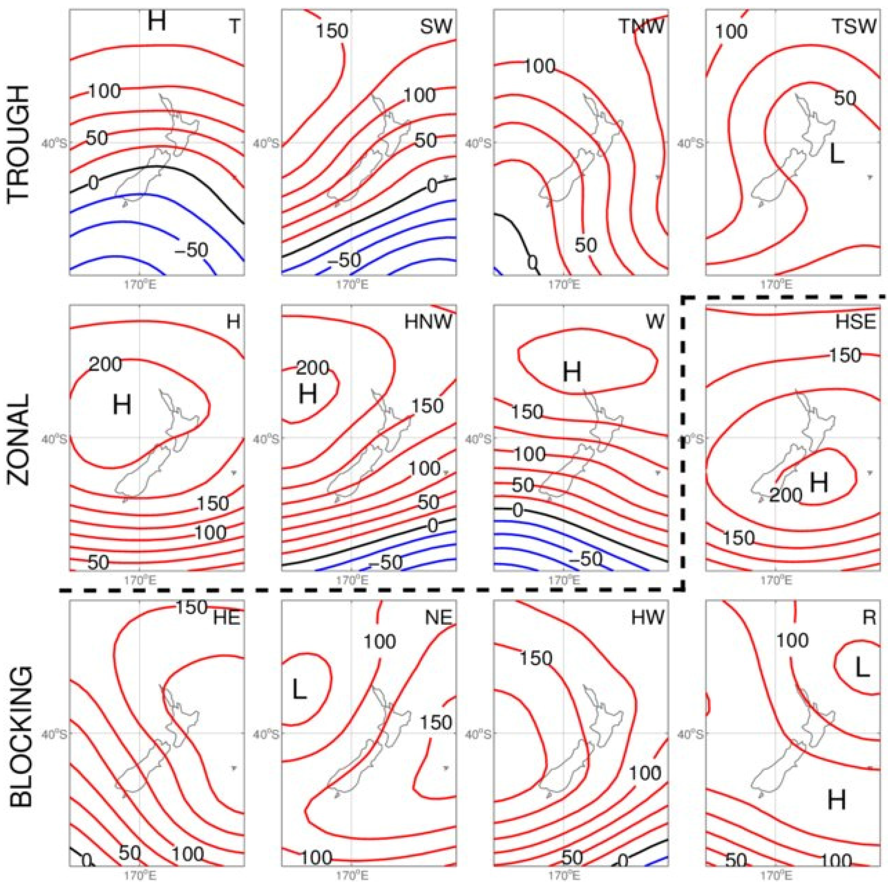
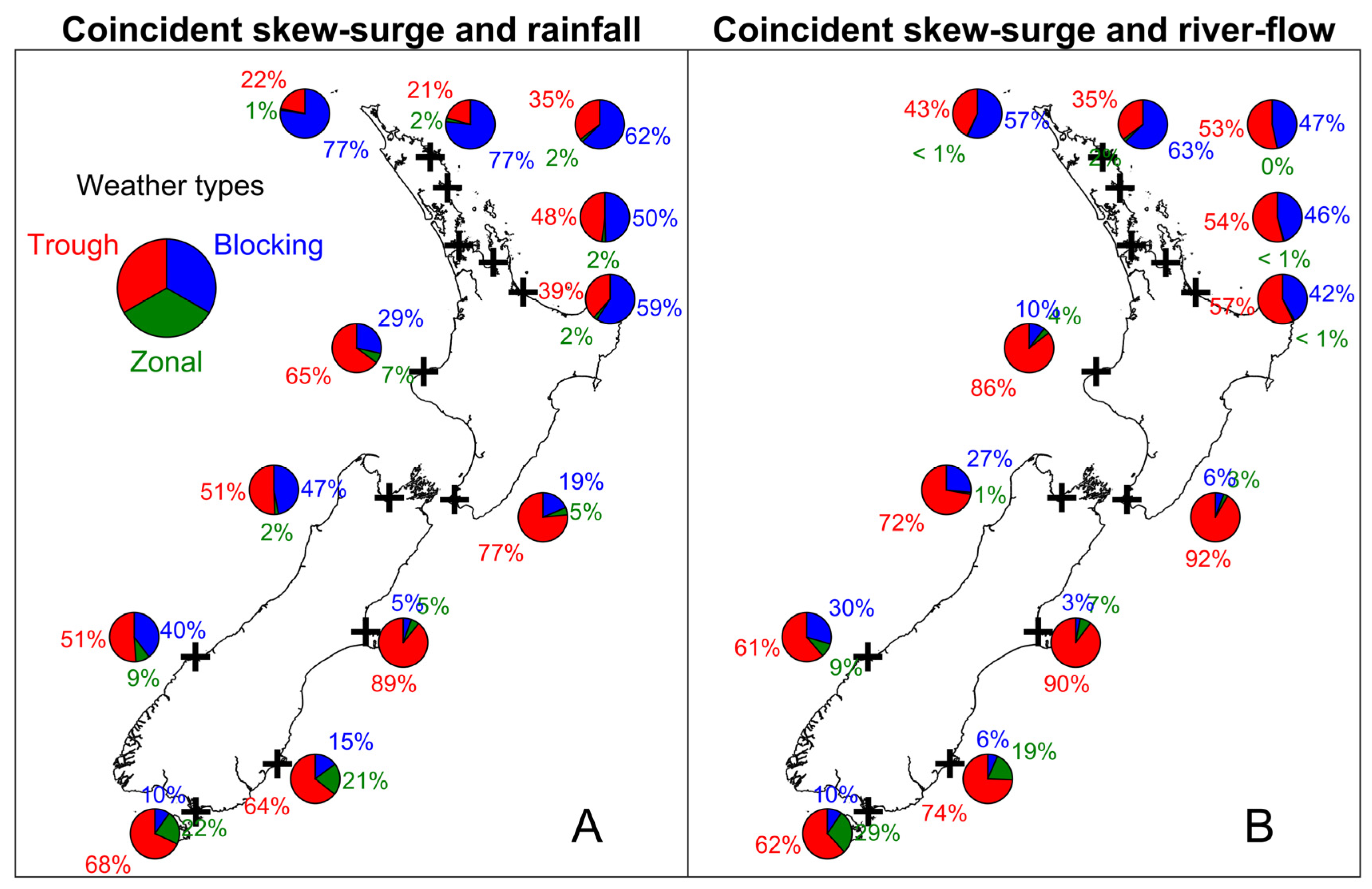
3.2. Weather Types Driving Patterns of Dependence

Figure 10 shows the distribution of Kidson (2000) weather types (Figure 3) associated with coincident skew-surge and rainfall, and skew-surge and river-flow events. Over much of New Zealand, trough weather regimes are the most common extreme event drivers (Figure 10). Troughs that cause extreme skew-surge events are associated with storm centers that tracked eastwards across NZ, usually across or south of the South Island and always south of the northernmost tip of NZ [24].
Coincident events located on the northeast coast of the North Island were associated with a higher proportion of blocking weather types (Figure 3). Blocking weather types are low-pressure systems that track from north of NZ and intensify next to a blocking high-pressure system lying east of NZ [29].
Table 2 provides information on site location, Kendall’s τ for the four dependence cases analyzed (Figure 4), and dominant weather types (Figure 10) at each sea-level recorder location. Although we have only plotted significant correlations (p-value ≤ 0.05) in the figures of the paper, for completeness, we have included τ in Table 2 even where the significance of the Kendall’s rank correlations did not meet the significance criterion. In this way, we can determine a more complete spatial relationship between τ and weather type. Significant correlations are given in underlined font and vice versa. Furthermore, for SS/F cases where no correlations could be identified within 30 km of the sea-level gauge location (no close river-flow records), we also extended the sampling radius to 100 km to complete the table (shown in italics font).
Coincident skew-surge and rainfall events were dominantly associated with blocking weather types on the northeast coast of the North Island and with trough weather types elsewhere. Nelson is also quite strongly influenced by blocking weather patterns, with 47% dominance (not shown). Coincident skew-surge and river-flow events showed a similar pattern, although trough weather types were also dominant in three of five locations on the northeast coast of the North Island, but only weakly so (<60%), and so were nearly equally matched by the occurrence of blocking weather types (not shown).
The median τ (all locations) was greater for coincident skew-surge and rainfall than coincident skew-surge and river-flow cases. The results in Table 2 are based on ± 1-day lag—it makes intuitive sense that correlations between skew-surge and rainfall would be higher than those between skew-surge and river-flow within a ± 1-day lag, since both skew-surge and rainfall may be driven by coincident weather systems, and river-flow can be expected to peak with some lag after a rainfall event.
The median τ correlation strength was higher during blocking weather types for rainfall and river-flow conditional on pre-existing extreme skew-surge cases (SS/R|SS, SS/F|SS), but was higher during trough weather types when skew-surge was conditional on pre-existing extreme rainfall or river-flow cases (SS/R|R, SS/F|F) (Table 2).
These patterns are consistent with our expectations of the synoptic types included in each regime. The trough group includes patterns which would bring wet, cool, and cloudy conditions to much of the country. The blocking group has anomalous northerly flow over much of the country, leading to milder conditions, whereas the NE and R classes (Figure 3) would bring strong winds and precipitation to the north and east of the North Island [29].

4. Discussion

The trough, zonal, and blocking groups account for 38%, 25%, and 37% of synoptic situations, respectively [29], but we found most coincident extreme events to be dominated by trough and blocking patterns. These observations are consistent with other studies. Griffiths [33] found that blocking weather types dominated extreme rainfall on the north and east coasts of New Zealand, and trough weather systems elsewhere (Figure 3) [33]. These findings are like those of Stephens et al. [24] for skew-surge. Given these observations for the individual drivers, it makes sense that blocking weather types were over-represented in coincident events on the northeast coast of New Zealand, and trough weather types elsewhere (Figure 10).
A synoptic climatological approach used to be largely of qualitative value, in that it helps the interpretation of why particularly climatic anomalies have been observed over the course of a month or season [29]. However, the statistical characterization of weather-types has more recently been used to create hindcasts of wave [36] and storm surge [37] conditions, and to simulate climate change projections of extreme storm surge [37]. Furthermore, knowledge of the spatial clustering of extreme skew-surge and rainfall or river-flow events is useful [24]—to understand and manage their risk exposure, central government agencies, environmental and emergency managers, and the insurance and financial sectors all require knowledge of the likely frequency and magnitude of extreme weather-related events and their clustering in time and space [24]. For example, our results show that emergency managers on the northeast coast of New Zealand or near Nelson should pay particular attention to forecasts of blocking weather types, knowing that these weather types drive coincident extreme skew-surge and rainfall/river-flow events.
We considered the dependence of meteorologically-driven coastal-hazard drivers as a first step toward understanding compound coastal flooding events. Our results show that the dependence between extreme skew-surge and river-flow is relatively weak in New Zealand compared to some locations internationally. For example, [22] identified several locations where the dependence between annual maxima of discharge and skew-surge had τ > 0.4, although many locations had no significant dependence. For New Zealand, we found very few locations with τ > 0.3 (e.g., Figure 4 and Figure 5) for any of the four cases analyzed (Table 1).
Ward et al. [22] found that the highest dependence (τ) over all time-lags (from −5 to +5 days) was higher than for the 0-day time-lag. Our dependence analysis has focused mainly on paired observations within ± 1-day of an extreme event, based on the assumption that the driver peaks will be closely spaced in time. This was generally found to be true, particularly for the skew-surge/rainfall (SS/R) situation. However, in the skew-surge/river-flow (SS/F) case, the dependence was often stronger when river-flow peak lagged skew-surge peak by about 2 days (Figure 9 and Supplementary Figures). Storm surge events are relatively short-lived (≤24 h) in New Zealand [24], so a lag of >1 day could substantially reduce compound flooding from coastal and fluvial events. This study has focused on the dependence between meteorological drivers, but not the mechanisms of coastal flooding, for which lags will be important along with local topographic characteristics that control how skew-surge and river-flow interact.
In addition, the tide is another important driver of coastal flooding. In New Zealand, the high-tide range is larger than skew-surge height, and the tide plays an important role in the timing of extreme storm-tide sea levels (storm-tide = tide + surge [24,38]). The tide is uncorrelated with skew-surge, rainfall, or river-flow, and so dependence measures between storm-tide sea levels and rainfall or river-flow are likely to be lower than for skew-surge. Therefore, fluvial flooding coinciding with very high tides—irrespective of surge—may be a stronger driver of compound flooding events in New Zealand and in other parts of the world. Nevertheless, we note that there was often significant positive dependence between SS/F pairs within ±1-day in close proximity to the sea-level gauge (Figure 4, Figure 5, Figure 6, Figure 7 and Figure 8). This implies that if a high tide should coincide with a large skew-surge, there is a statistically significant probability of a large river-flow also (and vice versa), leading to a compound flooding event. This is a topic for further investigation in NZ and elsewhere.
The positive dependence observed between skew-surge/rainfall and skew-surge/river-flow indicates that more attention to compound events is warranted when undertaking coastal-flood modelling in New Zealand. Compound flooding effects are highly locally dependent on the geometry of the estuary and the timing of the surge with respect to peak river discharge [12], and the prediction of compound flood impacts generally requires calibrated hydrodynamic models [9,10,12]. Boundary-condition scenarios to force the models can be derived from joint-probability models, e.g., [39,40,41], and meta-models can be trained to obtain the computational efficiency required to assess impacts from a multitude of compound event combinations, e.g., [42,43,44].

5. Conclusions

We used sea-level, rainfall, and river-flow measurements to assess the dependence of (1) extreme skew-surge and extreme rainfall and (2) extreme skew-surge and extreme river-flow in New Zealand. We identified the weather types driving regional patterns of dependence. The dependence was measured using Kendall’s rank correlation coefficient (τ) and was considered significant for p-value ≤ 0.05.
We found that (1) skew-surge and rainfall and (2) skew-surge and river-flow are significantly, but not strongly, correlated in NZ. When spatially averaged to within 30 km of the sea-level gauge (skew-surge) location, the correlation was generally significant and positive, but weak (τ < 0.3). This implies that compound events do occur in New Zealand, but with variability in the relative magnitudes of the drivers—very large skew-surges do not always coincide with very large rainfall or river-flow (and vice versa), but there is some correlation.
Trough weather types were the dominant driver of individual and coincident extreme events. Blocking weather types were associated with the highest extreme skew-surge and rainfall events along the northeast coast of the North Island and, consequently, were associated with a high proportion of coincident skew-surge/rainfall and skew-surge/river-flow events there. These findings have important implications for flood management, emergency response, and the insurance sector because impacts and losses may be spatially correlated—damage could be reduced by early preparation in specific locations in response to forecasts of particular weather types.
We focused on meteorologically-forced coastal-hazard drivers, but flooding impacts will also depend on the tidal height, which is uncorrelated with skew-surge, rainfall, or river-flow. The high-tide range is larger than skew-surge height in New Zealand, and so storm-tide sea levels are likely to have reduced dependence measures with rainfall or river-flow dependence—this is a topic for future research both in New Zealand and globally.

Supplementary Materials

The following supporting information can be downloaded at: https://www.mdpi.com/article/10.3390/jmse10121818/s1, Supplementary Materials: Skew-surge and rainfall (SS/R).

Author Contributions

S.A.S. conceived, performed the analyses, and wrote the paper. W.W. was involved in the study design. W.W. provided R code, which was trialed early in the analysis, and provided review. All authors have read and agreed to the published version of the manuscript.

Funding

Scott Stephens acknowledges funding from the NZ SeaRise Programme (Ministry of Business Innovation and Employment Contract: RTVU1705). Wenyan Wu acknowledges support from the Australian Research Council via the Discovery Early Career Researcher Award (DE210100117).

Data Availability Statement

Some of the sea-level records used for the work are available from the Global Sea Level Observing System website run by the University of Hawaii Sea Level Center. Other records are privately owned and permission for use may be sought by direct request to Land Information New Zealand. The rainfall data are available from NIWA at https://niwa.co.nz/climate/our-services/obtaining-climate-data-from-niwa (accessed on 1 November 2022). There is no single open-access river-flow database in New Zealand. Some river-flow data is available from NIWA by request, whereas most of the data was obtained for single use by permission from various Regional Councils.

Acknowledgments

Trevor Carey-Smith, Kathy Walter, and Alex Vincent of NIWA assisted with data supply and analysis. Thanks to three anonymous reviewers, whose review helped to improve the manuscript. Sea-level data were obtained from NIWA and from various port companies and regional councils in New Zealand. River-flow data were obtained from NIWA and from various regional councils in New Zealand.

Conflicts of Interest

The authors declare no conflict of interest.

References

  1. Haigh, I.D.; Wadey, M.P.; Wahl, T.; Ozsoy, O.; Nicholls, R.J.; Brown, J.M.; Horsburgh, K.; Gouldby, B. Spatial and temporal analysis of extreme sea level and storm surge events around the coastline of the UK. Sci. Data 2016, 3, 160107. [Google Scholar] [CrossRef] [PubMed] [Green Version]
  2. Needham, H.F.; Keim, B.D.; Sathiaraj, D. A review of tropical cyclone-generated storm surges: Global data sources, observations, and impacts. Rev. Geophys. 2015, 53, 545–591. [Google Scholar] [CrossRef]
  3. Lagmay, A.M.F.; Agaton, R.P.; Bahala, M.A.C.; Briones, J.B.L.T.; Cabacaba, K.M.C.; Caro, C.V.C.; Dasallas, L.L.; Gonzalo, L.A.L.; Ladiero, C.N.; Lapidez, J.P.; et al. Devastating storm surges of Typhoon Haiyan. Int. J. Disaster Risk Reduct. 2015, 11, 1–12. [Google Scholar] [CrossRef]
  4. Wahl, T.; Haigh, I.D.; Nicholls, R.J.; Arns, A.; Dangendorf, S.; Hinkel, J.; Slangen, A.B.A. Understanding extreme sea levels for broad-scale coastal impact and adaptation analysis. Nat. Commun. 2017, 8, 16075. [Google Scholar] [CrossRef] [Green Version]
  5. Jongman, B.; Ward, P.J.; Aerts, J.C.J.H. Global exposure to river and coastal flooding: Long term trends and changes. Glob. Environ. Chang. 2012, 22, 823–835. [Google Scholar] [CrossRef]
  6. Hinkel, J.; Lincke, D.; Vafeidis, A.T.; Perrette, M.; Nicholls, R.J.; Tol, R.S.J.; Marzeion, B.; Fettweis, X.; Ionescu, C.; Levermann, A. Coastal flood damage and adaptation costs under 21st century sea-level rise. Proc. Natl. Acad. Sci. USA 2014, 111, 3292–3297. [Google Scholar] [CrossRef] [Green Version]
  7. Hallegatte, S.; Green, C.; Nicholls, R.J.; Corfee-Morlot, J. Future flood losses in major coastal cities. Nat. Clim. Chang. 2013, 3, 802–806. [Google Scholar] [CrossRef]
  8. Paulik, R.; Stephens, S.A.; Bell, R.G.; Wadhwa, S.; Popovich, B. National-Scale Built-Environment Exposure to 100-Year Extreme Sea Levels and Sea-Level Rise. Sustainability 2020, 12, 1513. [Google Scholar] [CrossRef] [Green Version]
  9. Paprotny, D.; Vousdoukas, M.I.; Morales-Nápoles, O.; Jonkman, S.N.; Feyen, L. Pan-European hydrodynamic models and their ability to identify compound floods. Nat. Hazards 2020, 101, 933–957. [Google Scholar] [CrossRef] [Green Version]
  10. Bermudez, M.; Farfan, J.F.; Willems, P.; Cea, L. Assessing the Effects of Climate Change on Compound Flooding in Coastal River Areas. Water Resour. Res. 2021, 57, e2020WR029321. [Google Scholar] [CrossRef]
  11. Moftakhari, H.R.; Salvadori, G.; AghaKouchak, A.; Sanders, B.F.; Matthew, R.A. Compounding effects of sea level rise and fluvial flooding. Proc. Natl. Acad. Sci. USA 2017, 114, 9785–9790. [Google Scholar] [CrossRef] [PubMed] [Green Version]
  12. Maskell, J.; Horsburgh, K.; Lewis, M.; Bates, P. Investigating River–Surge Interaction in Idealised Estuaries. J. Coast. Res. 2014, 30, 248–259. [Google Scholar] [CrossRef]
  13. Wu, W.; Westra, S.; Leonard, M. Estimating the probability of compound floods in estuarine regions. Hydrol. Earth Syst. Sci. 2021, 25, 2821–2841. [Google Scholar] [CrossRef]
  14. Leonard, M.; Westra, S.; Phatak, A.; Lambert, M.; van den Hurk, B.; McInnes, K.; Risbey, J.; Schuster, S.; Jakob, D.; Stafford-Smith, M. A compound event framework for understanding extreme impacts. Wiley Interdiscip. Rev. Clim. Chang. 2014, 5, 113–128. [Google Scholar] [CrossRef]
  15. Zscheischler, J.; Westra, S.; van den Hurk, B.; Seneviratne, S.I.; Ward, P.J.; Pitman, A.; AghaKouchak, A.; Bresch, D.N.; Leonard, M.; Wahl, T.; et al. Future climate risk from compound events. Nat. Clim. Chang. 2018, 8, 469–477. [Google Scholar] [CrossRef]
  16. Bevacqua, E.; De Michele, C.; Manning, C.; Couasnon, A.; Ribeiro, A.F.S.; Ramos, A.M.; Vignotto, E.; Bastos, A.; Blesić, S.; Durante, F.; et al. Guidelines for Studying Diverse Types of Compound Weather and Climate Events. Earth’s Future 2021, 9, e2021EF002340. [Google Scholar] [CrossRef]
  17. Nasr, A.A.; Wahl, T.; Rashid, M.M.; Camus, P.; Haigh, I.D. Assessing the dependence structure between oceanographic, fluvial, and pluvial flooding drivers along the United States coastline. Hydrol. Earth Syst. Sci. 2021, 25, 6203–6222. [Google Scholar] [CrossRef]
  18. Wahl, T.; Jain, S.; Bender, J.; Meyers, S.D.; Luther, M.E. Increasing risk of compound flooding from storm surge and rainfall for major US cities. Nat. Clim. Chang. 2015, 5, 1093–1097. [Google Scholar] [CrossRef]
  19. Wu, W.; McInnes, K.; O’Grady, J.; Hoeke, R.; Leonard, M.; Westra, S. Mapping Dependence Between Extreme Rainfall and Storm Surge. J. Geophys. Res. Ocean. 2018, 123, 2461–2474. [Google Scholar] [CrossRef]
  20. Zheng, F.; Westra, S.; Sisson, S.A. Quantifying the dependence between extreme rainfall and storm surge in the coastal zone. J. Hydrol. 2013, 505, 172–187. [Google Scholar] [CrossRef]
  21. Santos, V.M.; Wahl, T.; Jane, R.; Misra, S.K.; White, K.D. Assessing compound flooding potential with multivariate statistical models in a complex estuarine system under data constraints. J. Flood Risk Manag. 2021, 14, e12749. [Google Scholar] [CrossRef]
  22. Ward, P.J.; Couasnon, A.; Eilander, D.; Haigh, I.D.; Hendry, A.; Muis, S.; Veldkamp, T.I.E.; Winsemius, H.C.; Wahl, T. Dependence between high sea-level and high river discharge increases flood hazard in global deltas and estuaries. Environ. Res. Lett. 2018, 13, 084012. [Google Scholar] [CrossRef]
  23. Kendall, M.G. A New measure of rank correlation. Biometrika 1938, 30, 81–93. [Google Scholar] [CrossRef]
  24. Stephens, S.A.; Bell, R.G.; Haigh, I.D. Spatial and temporal analysis of extreme storm-tide and skew-surge events around the coastline of New Zealand. Nat. Hazards Earth Syst. Sci. 2020, 20, 783–796. [Google Scholar] [CrossRef] [Green Version]
  25. Batstone, C.; Lawless, M.; Tawn, J.; Horsburgh, K.; Blackman, D.; McMillan, A.; Worth, D.; Laeger, S.; Hunt, T. A UK best-practice approach for extreme sea-level analysis along complex topographic coastlines. Ocean Eng. 2013, 71, 28–39. [Google Scholar] [CrossRef]
  26. Williams, J.; Horsburgh, K.J.; Williams, J.A.; Proctor, R.N.F. Tide and skew surge independence: New insights for flood risk. Geophys. Res. Lett. 2016, 43, 6410–6417. [Google Scholar] [CrossRef] [Green Version]
  27. Merrifield, M.A.; Genz, A.S.; Kontoes, C.P.; Marra, J.J. Annual maximum water levels from tide gauges: Contributing factors and geographic patterns. J. Geophys. Res.-Ocean. 2013, 118, 2535–2546. [Google Scholar] [CrossRef]
  28. Coles, S. An Introduction to Statistical Modeling of Extreme Values; Springer: London, UK; New York, NY, USA, 2001; p. 208. [Google Scholar]
  29. Kidson, J.W. An analysis of New Zealand synoptic types and their use in defining weather regimes. Int. J. Climatol. 2000, 20, 299–316. [Google Scholar] [CrossRef]
  30. Bennet, M.J.; Kingston, D.G. Spatial patterns of atmospheric vapour transport and their connection to drought in New Zealand. Int. J. Climatol. 2022, 42, 5661–5681. [Google Scholar] [CrossRef]
  31. Pohl, B.; Sturman, A.; Renwick, J.; Quénol, H.; Fauchereau, N.; Lorrey, A.; Pergaud, J. Precipitation and temperature anomalies over Aotearoa New Zealand analysed by weather types and descriptors of atmospheric centres of action. Int. J. Climatol. 2022. [Google Scholar] [CrossRef]
  32. Porhemmat, R.; Purdie, H.; Zawar-Reza, P.; Zammit, C.; Kerr, T. The influence of atmospheric circulation patterns during large snowfall events in New Zealand’s Southern Alps. Int. J. Climatol. 2021, 41, 2397–2417. [Google Scholar] [CrossRef]
  33. Griffiths, G. Drivers of extreme daily rainfalls in New Zealand. Weather Clim. 2011, 31, 24–49. [Google Scholar] [CrossRef]
  34. Renwick, J.A. Kidson’s Synoptic Weather Types and Surface Climate Variability over New Zealand. Weather Clim. 2011, 31, 3–23. [Google Scholar] [CrossRef]
  35. Ackerley, D.; Lorrey, A.; Renwick, J.A.; Phipps, S.J.; Wagner, S.; Dean, S.; Singarayer, J.; Valdes, P.; Abe-Ouchi, A.; Ohgaito, R.; et al. Using synoptic type analysis to understand New Zealand climate during the Mid-Holocene. Clim. Past 2011, 7, 1189–1207. [Google Scholar] [CrossRef] [Green Version]
  36. Camus, P.; Menendez, M.; Mendez, F.J.; Izaguirre, C.L.; Espejo, A.; Canovas, V.; Perez, J.; Rueda, A.; Losada, I.J.; Medina, R. A weather-type statistical downscaling framework for ocean wave climate. J. Geophys. Res.-Ocean. 2014, 119, 7389–7405. [Google Scholar] [CrossRef] [Green Version]
  37. Cagigal, L.; Rueda, A.; Castanedo, S.; Cid, A.; Perez, J.; Stephens, S.A.; Coco, G.; Méndez, F.J. Historical and future storm surge around New Zealand: From the 19th century to the end of the 21st century. Int. J. Climatol. 2020, 40, 1512–1525. [Google Scholar] [CrossRef]
  38. Stephens, S.A.; Bell, R.G.; Lawrence, J. Developing signals to trigger adaptation to sea-level rise. Environ. Res. Lett. 2018, 13, 104004. [Google Scholar] [CrossRef]
  39. Heffernan, J.E.; Tawn, J.A. A conditional approach for multivariate extreme values. J. R. Stat. Soc. Ser. B-Stat. Methodol. 2004, 66, 497–530. [Google Scholar] [CrossRef]
  40. Wahl, T.; Mudersbach, C.; Jensen, J. Assessing the hydrodynamic boundary conditions for risk analyses in coastal areas: A stochastic storm surge model. Nat. Hazards Earth Syst. Sci. 2011, 11, 2925–2939. [Google Scholar] [CrossRef]
  41. Wahl, T.; Mudersbach, C.; Jensen, J. Assessing the hydrodynamic boundary conditions for risk analyses in coastal areas: A multivariate statistical approach based on Copula functions. Nat. Hazards Earth Syst. Sci. 2012, 12, 495–510. [Google Scholar] [CrossRef]
  42. Malde, S.; Wyncoll, D.; Oakley, J.; Tozer, N.; Gouldby, B. Applying emulators for improved flood risk analysis. E3S Web Conf. 2016, 7, 04002. [Google Scholar] [CrossRef] [Green Version]
  43. Wyncoll, D.; Gouldby, B. Integrating a multivariate extreme value method within a system flood risk analysis model. J. Flood Risk Manag. 2013, 8, 145–160. [Google Scholar] [CrossRef] [Green Version]
  44. Gouldby, B.; Méndez, F.J.; Guanche, Y.; Rueda, A.; Mínguez, R. A methodology for deriving extreme nearshore sea conditions for structural design and flood risk analysis. Coast. Eng. 2014, 88, 15–26. [Google Scholar] [CrossRef]
Figure 1. Location of rainfall (blue), river flow (green), and sea level (red) records used. Sea level recorder locations 1–12 are labelled.
Jmse 10 01818 g001
Figure 2. Example of a single timeseries of skew-surge and rainfall for which Kendall’s τ was calculated for the SS/R|SS case (τ = 0.19 and p-value < 0.05). This example shows maximum daily-accumulated rainfall within ±1-day (lag). (A) Location of sea-level record (site 5, Auckland, Figure 1), plotted in the red triangle, and rainfall record, plotted in the blue circle. (B) Timeseries of skew-surge peaks-over-threshold (red triangles) and matching maximum daily-accumulated rainfall within ±1-day (blue circles). The rainfall record does not span the full duration of the sea-level record. (C) Scatter plot of the matched skew-surge and rainfall (for the period of overlap). (D) Scatter plot of the matched skew-surge and rainfall using log-log axes.
Jmse 10 01818 g002
Figure 3. The twelve Kidson weather types, shown as average patterns of 1000 hPa geopotential height (analogous to mean sea-level pressure). Contours mark 1000 hPa geopotential height anomaly in hPa. Names for the types are indicated in the top right of each panel. Source: Ackerley, et al. [35] distributed under the Creative Commons Attribution 3.0 License. The three regimes are indicated at the left: the top row is the trough regime, the first three in the second row are the zonal regime, and the rest form the blocking regime. See Kidson [29] for further details.
Jmse 10 01818 g003
Figure 4. Kendall’s rank correlation coefficient τ (color scale) averaged within 30 km of sea-level gauge for four cases (Table 1). Only correlations with a p-value of ≤0.05 were plotted; hence, not all cases are represented at all sites.
Jmse 10 01818 g004
Figure 5. Kendall’s rank correlation coefficient τ (color scale) calculated between skew-surge measured at Auckland and individual rainfall and river-flow records. (A) τ for skew-surge and rainfall, with rainfall conditional on extreme skew-surge; (B) τ for skew-surge and rainfall, with skew-surge conditional on extreme rainfall, (C) τ for skew-surge and river-flow, with river-flow conditional on extreme skew-surge, (D) τ for skew-surge and river-flow, with skew-surge conditional on extreme river-flow.
Jmse 10 01818 g005
Figure 6. Kendall’s rank correlation coefficient τ (color scale) calculated between skew-surge measured at Wellington and individual rainfall and river-flow records. (A) τ for skew-surge and rainfall, with rainfall conditional on extreme skew-surge; (B) τ for skew-surge and rainfall, with skew-surge conditional on extreme rainfall, (C) τ for skew-surge and river-flow, with river-flow conditional on extreme skew-surge, (D) τ for skew-surge and river-flow, with skew-surge conditional on extreme river-flow.
Jmse 10 01818 g006
Figure 7. Kendall’s rank correlation coefficient τ (color scale) calculated between skew-surge measured at Lyttelton and individual rainfall and river-flow records. (A) τ for skew-surge and rainfall, with rainfall conditional on extreme skew-surge; (B) τ for skew-surge and rainfall, with skew-surge conditional on extreme rainfall, (C) τ for skew-surge and river-flow, with river-flow conditional on extreme skew-surge, (D) τ for skew-surge and river-flow, with skew-surge conditional on extreme river-flow.
Jmse 10 01818 g007
Figure 8. Kendall’s rank correlation coefficient τ (color scale) calculated between skew-surge measured at Dunedin and individual rainfall and river-flow records. (A) τ for skew-surge and rainfall, with rainfall conditional on extreme skew-surge; (B) τ for skew-surge and rainfall, with skew-surge conditional on extreme rainfall, (C) τ for skew-surge and river-flow, with river-flow conditional on extreme skew-surge, (D) τ for skew-surge and river-flow, with skew-surge conditional on extreme river-flow.
Jmse 10 01818 g008
Figure 9. Lagged analysis Kendall’s rank correlation coefficient τ (color scale) calculated between skew-surge measured at Auckland and individual river-flow records. (A) SS/F|SS river-flow within ± 1-days of extreme skew-surge event; (B) SS/F|SS river-flow 2-days before extreme skew-surge event; (C) SS/F|SS river-flow 2-days after extreme skew-surge event; (D) SS/F|F skew-surge within ± 1-days of extreme river-flow event;€) SS/F|F skew-surge 2-days before extreme river-flow event; (F) SS/F|F skew-surge 2-days after extreme river-flow event.
Jmse 10 01818 g009
Figure 10. Pie charts showing weather type causing composite skew-surge, rainfall, and river-flow events. Skew-surge and rainfall events, >95th percentile. Skew-surge and river-flow events, >90th percentile. Colors refer to Kidson type: red = trough, green = zonal, and blue = blocking. Rainfall and coincident events chosen within 30 km of one another. (A) Coincident skew-surge and rainfall, (B) Coincident skew-surge and river-flow.
Jmse 10 01818 g010
Table 1. Description of the four dependence cases analyzed.
SymbolDescription
SS/R|SSSkew-surge and rainfall, with rainfall conditional on extreme skew-surge.
SS/R|RSkew-surge and rainfall, with skew-surge conditional on extreme rainfall.
SS/F|SSSkew-surge and river-flow, with river-flow conditional on extreme skew-surge.
SS/F|FSkew-surge and river-flow, with skew-surge conditional on extreme river-flow.
Table 2. Spatially-averaged Kendall’s τ for the four dependence cases analyzed using ± 1-day lag (Table 1, Figure 4) at each sea-level recorder location, and dominant weather types. Kendall’s τ: bold underlined = significant at p-value ≤ 0.05 using rainfall or river-flow records within 30 km radius of sea-level gauge; underlined not bold = significant at p-value ≤ 0.05 using river-flow records within 100 km radius; normal font = insignificant (p-value > 0.05); italics = insignificant (p-value > 0.05) and using river-flow records within 100 km. B = dominance of blocking weather type (including percentage of coincident events during blocking weather types), and T = dominance of trough weather type (including percentage of coincident events during trough weather types).
SiteLocationτ
SS/R|SS
τ
SS/F|SS
τ
SS/R|R
τ
SS/F|F
Coincident Skew-Surge and RainfallCoincident Skew-Surge and River-Flow
1. OpuaNorth Is northeast coast0.220.230.200.03B (77%)B (57%)
2. Marsden PointNorth Is northeast coast0.250.190.230.08B (77%)B (63%)
3. AucklandNorth Is northeast coast0.180.220.100.19B (62%)T (53%)
4. TararuNorth Is northeast coast0.170.210.110.17B (50%)T (54%)
5. MoturikiNorth Is northeast coast0.400.080.130.17B (59%)T (57%)
6. TaranakiNorth Is west coast0.01−0.030.260.07T (65%)T (86%)
7. NelsonSouth Is north coast0.190.170.170.11T (51%)T (72%)
8. WellingtonNorth Is south coast−0.070.020.160.05T (77%)T (92%)
9. LytteltonSouth Is east coast0.25−0.030.180.22T (89%)T (90%)
10. Jackson BaySouth Is west coast0.140.160.160.18T (51%)T (61%)
11. DunedinSouth Is east coast0.040.00−0.050.14T (64%)T (74%)
12. Dog IslandSouth Is south coast0.060.040.080.09T (68%)T (62%)
Median τ, all weather types0.170.120.160.12
Median τ, blocking weather type dominance0.220.210.130.06
Median τ, trough weather type dominance0.060.060.160.15
Publisher’s Note: MDPI stays neutral with regard to jurisdictional claims in published maps and institutional affiliations.

