Article

Water Circulation, Temperature, Salinity, and pCO2 Distribution in the Surface Layer of the East Kamchatka Current

V.I. Il’ichev Pacific Oceanological Institute, 690041 Vladivostok, Russia
*
Author to whom correspondence should be addressed.
J. Mar. Sci. Eng. 2022, 10(11), 1787; https://doi.org/10.3390/jmse10111787
Submission received: 6 October 2022 / Revised: 17 November 2022 / Accepted: 17 November 2022 / Published: 20 November 2022
(This article belongs to the Section Chemical Oceanography)

Abstract

:
The ship-borne observations of the temperature, salinity, pCO2 (1995–2020) and satellite geostrophic velocity fields, SST, and chlorophyll concentration are used to identify the factors that determine the spatio-temporal variability of seawater parameters on the western boundary of the subarctic North Pacific. In winter, the surface layer of the East Kamchatka Current (EKC) was characterized by two types of water: the waters with a negative temperature (−1.0–−0.5 °C) and salinity of 32.4–32.9 and waters with a positive temperature (0.4–1.7 °C) and salinity of 33.0–33.1. The source of water with negative (positive) temperature and decreased (increased) salinity for the EKC zone is the Bering Sea shelf (Aleutian Basin). The surface waters in the eastern Kamchatka area in winter were close to gas equilibrium with the atmosphere or supersaturated with carbon dioxide (pCO2 = 380–460 µatm). In summer, extremely low pCO2 values (140–220 µatm) in the surface layer of the eastern Kamchatka and the northern Kuril Islands regions have been associated with the decreased salinity (32.1–32.6) of the waters. The distributions of the temperature, salinity, and pCO2 in the surface layer of the central Kuril Islands are determined by the location and intensity of the Kuril eddies and the EKC stream jets. The water mixing in the central Kuril Straits and the Kruzenshterna Bank area leads to increased salinity (33.2–33.4) and high values of pCO2 (480–670 µatm) in the surface layer of the EKC. The comparison of the pCO2 data collected in winter demonstrates an increase in pCO2 between 1998/2001 and 2018/2020 at about 50 µatm in the surface waters with a salinity of 33.0–33.1, which is in agreement with an increase in pCO2 in the atmosphere at 46 µatm (from 368 to 414 µatm) during this period.

1. Introduction

The water circulation of the subarctic North Pacific consists of a cyclonic gyre that encompasses the Gulf of Alaska and the northwestern Pacific and enters the Bering and Okhotsk Seas [1]. The Alaskan Stream and the East Kamchatka Current (EKC) are the northern and western boundary currents of the subarctic North Pacific (Figure 1). Portions of the Alaskan Stream flow through the Aleutian Passes and Near Strait and form a cyclonic circulation cell in the Bering Sea [2]. The EKC, flowing southwestward along the east coast of the Kamchatka Peninsula and the Kuril Islands, originates from a flow out of the Bering Sea waters through the Kamchatka Strait. The flow of the EKC in the western Bering Sea and the Kamchatka Strait is strong between November and April and relatively weak in June–September. The strong seasonality in the surface flow of the EKC can be explained by temporal changes in the wind stress over the northern and western Bering Sea continental slope [3,4]. Meanders and eddies are consistent features in the EKC region [5,6]. The EKC area is the main pathway of the Bering Sea origin water to the North Pacific. Enhanced EKC advection is accompanied by an increase in water temperature and decreasing ice area in the Okhotsk Sea in winter [7].
There is a lack of analyses of the EKC circulation in the western subarctic North Pacific. Previous studies have mainly addressed the East Kamchatka and Kuril anticyclonic eddies [7]. The study conducted during the joint Russia–Japan expedition showed significant spatial variability in the distribution of chemical parameters in the central Kuril Islands region in May–June 2000 [8]. The impact of the water circulation on the temperature, salinity, and chemical parameter distributions in the surface layer of the EKC area has not been described and discussed before.
Seawater carbon dioxide partial pressure (pCO2) (partial pressure of CO2 in the gas phase in equilibrium with the seawater) is one of the carbonate parameters of seawater that determines the direction and magnitude of the CO2 flux between the atmosphere and the ocean. pCO2 is an indicator of the physical and biogeochemical processes in seawater. The seasonal maps of pCO2 [9,10,11] demonstrate that the western subarctic Pacific is a source (sink) for atmospheric CO2 in winter (summer). The EKC area is a dynamically active region, which is characterized by strong tidal currents and water mixing in the Kuril Straits, the water supply from the Bering and Okhotsk Sea, eddy formation and migration [12], and enhanced biological activity in spring–summer [8]. These factors affect the temperature, salinity, and pCO2 distribution in the study area. The supply of the Okhotsk Sea and Bering Sea shelf water decreases temperature and salinity in the EKC zone in winter–spring. Due to tidal mixing in the Kuril Straits, the surface layer of the EKC is enriched in salinity and seawater pCO2. In winter (summer), the tidal mixing increases (decreases) the temperature in the surface layer due to the temperature maximum (minimum) in the intermediate (surface) layer. The phytoplankton bloom is accompanied by a decrease in seawater pCO2.
In this paper, we analyze the ship-borne and satellite–derived data collected in the zone of the EKC between 1995 and 2020. The processes that influence the spatial and temporal variability of temperature, salinity, and pCO2 in the study region are shown. The main emphasis is on the effect of water circulation on the distribution of salinity, temperature, and pCO2 of surface waters. First, we discuss the pCO2 distribution in the winter of 2003 and winter of 2013 during periods, respectively, with low temperature and salinity and increased temperature and salinity in the surface layer of the EKC zone. Then, we compare the data collected in 2003 and 2013 with the data obtained in the winter of 1998/2002, the winter of 2018, and the winter of 2020. To demonstrate the amplitude of the seasonal variability of pCO2 in the study area, the data collected in the summer of 1995, the summer of 1998, and the summer of 1999 are presented.

2. Materials and Methods

2.1. Sea Surface Heights, Geostrophic Velocities, SST, and Chlorophyll Concentration Data

Our study is based on data on the sea surface heights (SSHs) and geostrophic current velocities with a spatial resolution of 0.25° by 0.25° (for the study area of ~30 km in longitude and ~20 km in latitude) and a temporal resolution of 1 day obtained from satellite measurements (Copernicus database, http://marine.copernicus.eu, accessed on 10 April 2022) for the period from 1995 to 2020. The spatial and temporal variability of the chlorophyll concentration was investigated using data from the Aqua satellite with a spatial resolution of 4 km (http://oceancolor.gsfc.nasa.gov, accessed on 20 April 2022). The error value of satellite data for the SSH values measured from 2002 until the present is 1–2 cm at distances more than 20–40 km from the shoreline [13]. Based on the accepted SSH error value, the error of the geostrophic current velocities for the off-shore region is 3–6 cm/s.
The SST (Sea Surface Temperature) images (spatial resolution of 1 km) were provided by GHRSST (Group for High-Resolution Sea Surface Temperature) (PO.DAAC-GHRSST Level 4 MUR Global Foundation Sea Surface Temperature Analysis). The Argo float data (temperature, salinity) were provided by the National Oceanic and Atmospheric Administration (NOAA) (http://www.nodc.noaa.gov/argo, accessed on 15 May 2022) [14]. The data on wind directions and velocities, as well as sea-level atmospheric pressure, were obtained from the NOAA Earth System Research Laboratories (http://www.esrl.noaa.gov accessed on 15 April 2022, accessed on 15 April 2022).

2.2. Underway pCO2, Salinity, Temperature Observations and Air–Sea CO2 Flux Estimation

In this paper, we use ship-borne observations of temperature, salinity in the surface layer, seawater pCO2, and pCO2 in the atmosphere (pCO2atm) in the period from 1995 to 2020 [15,16,17,18,19] (https://www.ncei.noaa.gov/access/ocean-carbon-data-system/oceans/VOS_Program, accessed on 10 April 2022). The determination of seawater pCO2 in the surface layer was carried out in accordance with the procedure described in the manual for ocean CO2 measurements (SOP 5) [20]. The measurements were carried out underway (Figure 2). Seawater from the surface horizon (5–8 m) was continuously supplied to the gas equilibrator. The measurement of CO2 concentration in the gas phase was carried out using an NDIR CO2 analyzer. The accuracy of the pCO2sw measurements was ±1–3 µatm. The temperature and salinity measurements were carried out using a thermosalinograph manufactured by Sea-Bird company with a precision of 0.001 °C and 0.01, respectively [15].
The flux of carbon dioxide between the ocean and the atmosphere (F) was computed using the following equation:
F = K∙ΔpCO2
where ΔpCO2 is the difference in seawater and atmosphere pCO2, and K is the CO2 exchange coefficient determined by the product of CO2 solubility in seawater [21] and the coefficient of CO2 transfer through the seawater–atmosphere interface (gas transfer velocity). The gas transfer velocity (Kw) was calculated using the wind speed data (NCEP/NCAR reanalysis data) and the quadratic relationship between the Kw and wind speed (U) [22].
Kw = 0.31·U2∙(Sc/600)−0.5
The equation for calculating the Schmidt number (Sc) for CO2 was obtained from [23].

2.3. Calculation of the Seawater pCO2 Depth Profiles

To calculate the depth profiles of seawater pCO2 in the study region, we used hydrocast data (temperature, salinity, nutrients, total alkalinity, and dissolved inorganic carbon concentrations) collected in the northwestern Pacific in winter–spring 2010, 2012, and 2013. The data were provided by the National Center for Environmental Information (https://www.ncei.noaa.gov/access/ocean-carbon-data-system/oceans/GLODAPv2_2020, accessed on 15 May 2022) [24]. Nutrients (phosphate, nitrate, and silicate) were determined spectrophotometrically with a precision of 1–2%. The total alkalinity (TA) was determined by potentiometric titration in an open cell [20]. The dissolved inorganic carbon (DIC) was measured by a coulometer. DIC and TA were calibrated versus certified reference materials (CRMs) [20]. The repeatability of the DIC and TA measurements [20] was ±2–3 μmol kg−1. The seawater pCO2 values were computed from DIC–TA and nutrient data using the CO2SYS Program [25]. The carbonic acid dissociation constants of Mehrbach et al. [26], as refitted by Dickson and Millero [27], were used. The uncertainty in the computed pCO2 was about ±10 μatm.

3. Results

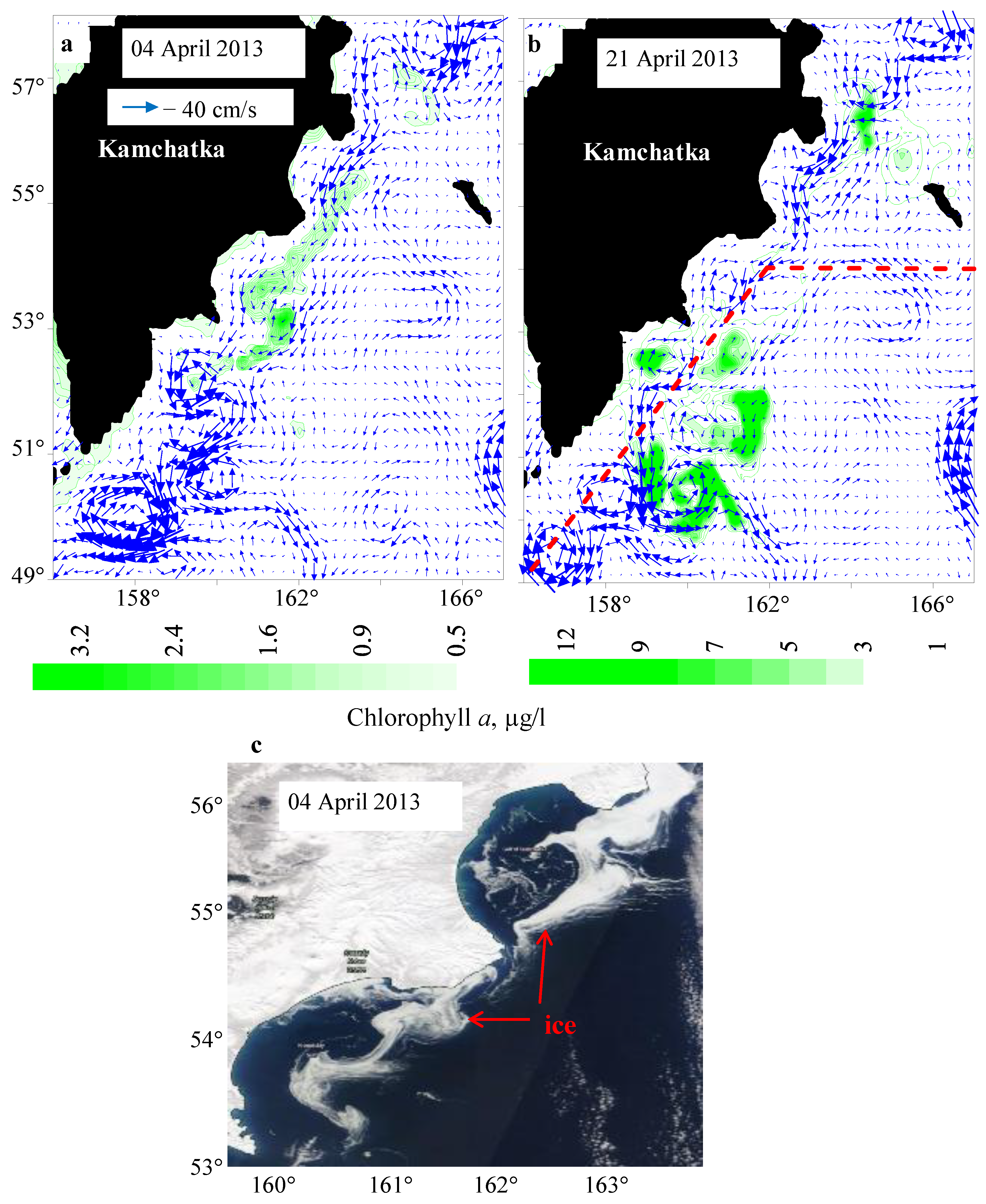
3.1. Water Circulation in the Study Area

The SSH, current velocity maps (February and March 2003, January and February 2013), and SST distributions in March 2003 and March 2013 are shown in Figure 3. Geostrophic velocity maps (Figure 3a–d) demonstrate the EKC running southwestward along the eastern Kamchatka and Kuril Islands with a velocity of 20–40 cm/s. In January 2013, two branches of the EKC in the Kuril Islands area were distinguished: coastal and off-shore branches (Figure 3c). In March 2003 and February 2013, only the off-shore branch of the EKC was observed (Figure 3b,d). In February 2003, in the central Kuril Islands area, the coastal water flow of the EKC, running parallel to the Nadezdy, Rickorda, and Diana straits (Rickorda Strait area) (Figure 3a), was detected. In February 2003 and February 2013, the formation of anticyclonic eddies occurred near the eastern Kamchatka (Kamchatka Eddies) (Figure 3a) and in the northern Kuril Islands region (Figure 3c). One month later (March 2003 and March 2013), the eddies moved off-shore and did not influence the water exchange between the coastal and the open Pacific Ocean (Figure 3b,d). In March 2003, the waters with negative SST occupied only the shore zone of eastern Kamchatka and the northern Kuril Islands (Figure 3e). In March 2013, the area with negative SST values extended as a wide strip from the Bering Strait to the southeast along the entire western boundary of the subarctic Pacific (Figure 3f).
In January–April 2013, the mesoscale anticyclonic eddy (45.0–46.8° N, 152–155° E) (Figure 3c,d) determined the water exchange between the coastal and open Pacific Ocean in the central Kuril Islands zone. The anticyclonic eddy advected the Kuril Island low-temperature coastal water to the pelagic part, resulting in a decrease in SST from about 1.5 °C to 0.5 °C in the central area of the western subarctic North Pacific (GHRSST data, https://worldview.earthdata.nasa.gov/, accessed on 20 April 2022).

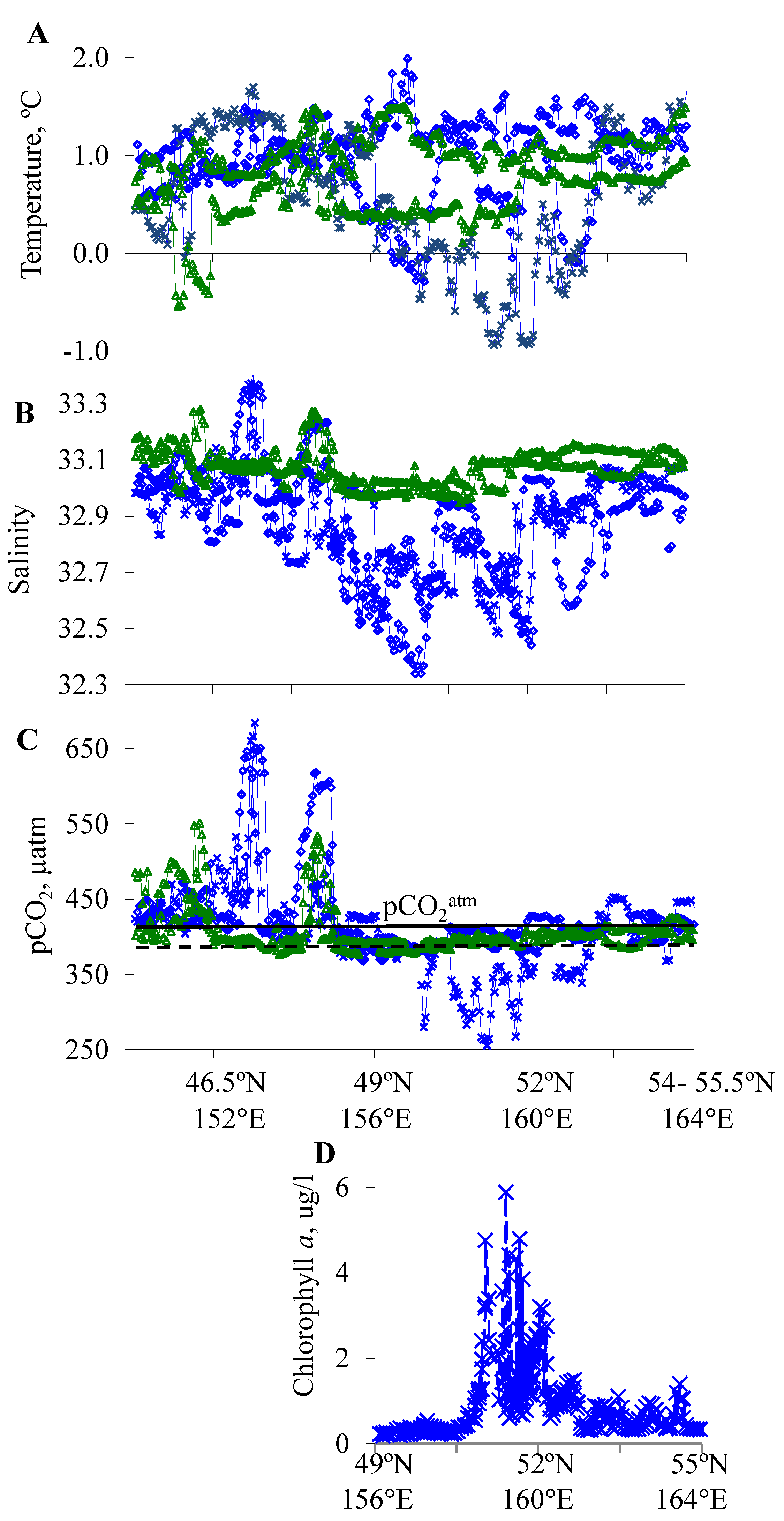
3.2. Distribution of Temperature, Salinity, and pCO2

3.2.1. East Kamchatka and North Kuril Areas

The distributions of temperature, salinity, and pCO2 in the eastern Kamchatka and northern Kuril Islands areas (48–54° N, 155–164° E) (Figure 4A–C) show that the surface waters in the EKC zone (156–162° E) in January–April 2013 were characterized by negative temperature (−0.9–−0.6 °C) and low salinity (32.4–32.9) compared to February and March 2003 (temperature of 0.4–1.2 °C and salinity of 33.0–33.1). In February–March 2003 and January–February 2013, seawater pCO2 was 385–410 µatm. The surface waters in the zone of eastern Kamchatka were slightly supersaturated with carbon dioxide relative to the atmosphere (pCO2atm = 370–376 µatm) in February and March 2003 and were close to gas equilibrium with the atmosphere in January and February 2013 (pCO2atm = 386–390 µatm).
According to Argo float data (2012–2020), the vertical water structure in the southwestern Bering Sea (57–59° N, 164–166° E) and near the eastern Kamchatka in the winter and early spring was characterized by a uniform temperature (0.5–1.5 °C) and salinity (32.9–33.1) in the 0–300/400 m layer. On some vertical profiles, the Bering Sea shelf water with a negative temperature (−1.5–0.5 °C) and salinity of 32.2–32.7 was observed in the 0–100 m layer. The water mixing induced by winter convection and wind, covering the upper layer to a depth of 300/400 m, should have led to a significant supersaturation of CO2 in the surface waters. However, in the winter of 2003 and the winter of 2013, the surface waters near the Kamchatka and northern Kuril Islands were only slightly oversaturated with CO2 relative to atmospheric CO2. Probably, intense gas exchange between the ocean and atmosphere reduced the seawater pCO2. Another important factor that reduces the seawater pCO2 in winter is a decrease in water temperature [28].
A significant reduction in pCO2 from 400 µatm on 16–18 February 2013 to 250–300 µatm on 21 April 2013 in the zone of eastern Kamchatka (Figure 4C) was related to spring phytoplankton bloom. The decrease in pCO2 during phytoplankton growth was accompanied by an increase in the concentration of chlorophyll a (Figure 4D). The distribution of chlorophyll a concentration (Figure 5a,b) and satellite images (Figure 3f and Figure 5c) demonstrate that spring bloom in early April 2013 was observed in waters with negative SST originating from the Bering Sea and was tied to the boundaries of ice fields. Two weeks later (15–21 April 2013), a high concentration of chlorophyll was noted at the boundaries of mesoscale anticyclones and the cyclones near southeastern Kamchatka (Figure 5b). Based on the pCO2 data, it is possible to estimate the consumption of DIC in seawater during photosynthesis.
For the western part of the subarctic North Pacific, the change in the carbonate parameters in the surface waters caused by the formation of carbonates is insignificant [29]. During the synthesis of organic matter, CO2 and nitrate are consumed, which is accompanied by a decrease in DIC and an increase in TA [30]. The changes in DIC, TA, and pCO2 during photosynthesis could be quantified using the Redfield ratio (C:N:P = 117:16:1) [31] and CO2SYS Program [25]. For the eastern Kamchatka area, a decrease in DIC concentration by 50 µmol L−1 and an increase in TA by 7 µmol L−1 during the phytoplankton bloom in early spring (t = 0 °C, S = 33.0, DIC = 2126 µmol L−1, TA = 2240 µmol L−1) lead to a decrease in pCO2 by 120 µatm (from 390 to 270 µatm). Therefore, to reduce pCO2 from 390 to 270 µatm in the EKC zone in April 2013, the DIC concentration had to decrease by 50 µmol L−1. The decline of the seawater pCO2 below the pCO2atm value (400 µatm, April 2013) causes a flux of CO2 from the atmosphere into seawater, which partially compensates for the reduced DIC and pCO2 due to phytoplankton growth. Applying Equations (1) and (2), we find that the average CO2 flux from the atmosphere to the ocean over the period under study (4–21 April 2013, wind speed of 5 m/s) was equal to 5 mmol C m−2 day−1. The increase in DIC in the upper 10 m layer of the study area due to the influx of CO2 from the atmosphere was approximately 10 µmol L−1. Therefore, the consumption of DIC related to phytoplankton growth was about 60 µmol L−1 (720 µg C L−1). In the period from 4 April to 21 April 2013, the concentration of chlorophyll increased by 5–6 µg L−1. The ratio between the decrease in the concentration of DIC and the increase in the concentration of chlorophyll a was equal to 120–144 (µg C/µg chlorophyll), without considering the loss of phytoplankton biomass and the decrease in the concentration of chlorophyll a due to phytoplankton mortality and zooplankton grazing.
In late January–early February 1999 and in March 1999 (Figure 6), the distributions of temperature and salinity in the EKC zone (49° N, 156° E–54° N, 162° N) were similar to those in January–February 2013 (Figure 4A,B). In these periods, near the eastern Kamchatka and the northern Kuril Islands, waters with low temperatures (−1–0 °C), decreased salinity (32.35–32.80), and pCO2 values of 390–420 µatm were observed. The surface layer of the Kamchatka Eddy (48.3–50.7° N, 157–159° E, SSH = 45 cm) was formed by water with negative temperature (−1 °C), low salinity (32.35), and pCO2 equal to 350 µatm (March 1999) (Figure 6). The source of water with a temperature of −1.0–−0.5 °C and a salinity of 32.0–32.5 for the EKC zone in the winter and early spring of 1999 and 2013 was the Bering Sea shelf. In February–March 2000 (Figure 6), February–March 2003 (Figure 4), February 2018, and February 2020 (Figure 7), the surface layer of the EKC was characterized by positive temperature (0.5–1.5 °C), a salinity of 33.0–33.1, and pCO2 values equal to 390–460 µatm. During these periods, the source of surface water for the EKC area was the Bering Sea deep basin (Aleutian Basin), characterized by a positive water temperature (1.0–2.0 °C) and a salinity of 33.0–33.2 in winter [32]. In February 2018, the surface water temperature in the northern Kuril and eastern Kamchatka region (155–159° E) was higher than in February 2020 (1.2 °C and 1.7 °C, respectively), but the salinity and pCO2 were similar to those observed in February 2020 (33.0 and 450–460 µatm) (Figure 7).
The water inflow from the Bering Sea into the Pacific Ocean through the Kamchatka Strait is enhanced in winter and determined by the wind stress along the continental slope of the Bering Sea [3]. In the winter of 1999 and winter of 2013, the low atmospheric pressure area (Aleutian Low) was located over the subarctic Pacific and southern Bering Sea zone. The eastern winds (10–12 m/s, monthly averaged speeds) over the central Bering Sea contributed to the intensification of the southwestern current along the western boundary of the Bering Sea [4] and the inflow of Bering shelf water into the EKC zone.
In winter 1998, winter 2000, winter 2003, winter 2018, and winter 2020, the Aleutian Low was located over the central subarctic Pacific. In the southern part of the Bering Sea, the northeastern winds with a speed of 4–8 m/s were dominated, and, as a result, the Aleutian Basin water with positive temperatures and salinity of 33.0–33.2 entered the EKC zone.
In summer, the EKC is weak, and the water dynamics at the western subarctic Pacific boundary are determined by mesoscale water circulation. In June 1995, July 1998, and July 1999, mesoscale (horizontal size 100–200 km) anticyclonic eddies were observed near the eastern Kamchatka, northern Kuril, and central Kuril Islands. In June 1995 and July 1998, the Kamchatka eddy was weak (the velocities at the margins were 20–40 cm/s). In July 1999, the Kamchatka eddy was intensified, its horizontal dimension was increased to 200 km, and the current velocities at its boundary were increased up to 70 cm/s.
The distributions of salinity and pCO2 across the Kamchatka eddy (July 1998, July 1999) and the eddy southeastern periphery (June 1995) (Figure 8A,B; 158–160° E) show that in summer the surface layer of the Kamchatka eddy was composed by low salinity (32.1–32.5) and low pCO2 (140–220 µatm) waters. In July 1999, low–salinity (32.1–32.6) and low pCO2 (160–200 µatm) Bering Shelf waters occupied the EKC zone from the eastern Kamchatka to the northern Kuril Islands.

3.2.2. Central Kuril Island Area

The distributions of temperature, salinity, and pCO2 in the central Kuril Islands region (45–48° N, 150–155° E) were related to water circulation. Increased salinity (33.1–33.3) and high pCO2 values (500–650 µatm) were observed in the Rickorda Strait zone (Figure 4B,C: 151–153° E) and Kruzenshterna Bank area (Figure 4B,C: 154–155° E), where due to tidal mixing, the surface water is enriched with pCO2. The Rickorda Strait area (Nadezdy, Rickorda, and Diana straits), with an average depth of 160–240 m, is characterized by high velocities of tidal currents (2–4 m/s), which contribute to tidal mixing and water transformation [33].
In February 2003, the coastal branch of the EKC was running southwestward along the Rickorda Strait zone (Figure 3a). During this period, in the region of the central Kuril Islands, the waters with a temperature of 0.8–1.2 °C, a salinity of 33.2–33.3, and a pCO2 of 500–550 µatm were observed. In March 2003, the coastal branch of the EKC was not noted (Figure 3b). The central Kuril area was characterized by decreased temperature (−0.5–0.5 °C), a salinity of 33.0–33.1, and a pCO2 equal to 390–430 µatm. The presence of Kuril Eddy (45.0–46.8° N, 152–155° E) in January–April 2013 (Figure 3c,d), which determines the water exchange between the coastal and pelagic parts of the western subarctic North Pacific, led to anomalously high pCO2 values (640–690 µatm) in the central Kuril area (Figure 4C: 152° E).
A principal feature of the western subarctic water structure is the sharp halocline/pycnocline at the bottom of the upper layer at about 100 m depth (Figure 9B). In winter, the halocline prevents the direct ventilation of the intermediate water layer, characterized by high concentrations of nutrients and DIC [29]. In the 100–200 m layer, pCO2 increased from 500 to 1400 µatm (Figure 9C). In the salinity range of 33.1–33.6, dependence (close to linear) of pCO2 on salinity is observed (Figure 9D). Vertical mixing will increase the salinity and a significant increase in pCO2 in the surface layer. Due to tidal mixing in the Kuril Straits, the halocline is destroyed, and the surface layer is enriched in salinity and seawater pCO2. In winter, the water mixing increases the temperature in the surface layer due to the maximum temperature in the intermediate layer (Figure 9A). In the surface layer at the western boundary of the subarctic North Pacific in the winter of 2003 and the winter of 2013, there is a tendency for pCO2 to increase from 380 to 660 µatm with an increase in salinity from 32.34 to 33.37.
Distributions of the temperature, salinity, and pCO2 in the surface waters of the central Kuril Islands in January–March 1999, February–March 2000, February 2018, and February 2020 (Figure 6 and Figure 7) were determined by the location and intensity of the Kuril eddies and the EKC stream jet. Increased values of pCO2 (450–480 µatm) in the Kruzenshterna Bank area (Figure 6C: 154–155° E) were observed in late January–early February 1999, March 2000, and February 2020. During these periods, the southwestward running the EKC stream jet (velocity of 50–60 cm/s) crossed the Kruzenshterna Bank. In March 1999 and February 2000, the velocities of the EKC decreased (20–25 cm/s), and the EKC stream jet was located eastward and southward of the Kruzenshterna Bank. As a result, in March 1999 and February 2000, in the Kruzenshterna Bank zone, the pCO2 was close to equilibrium with the atmosphere (365–375 µatm).
In late January–early February 1999 and March 2000, the water dynamics in the central Kuril area were determined by mesoscale anticyclonic circulation encompassing the Bussol and Rickorda Straits. The anticyclonic circulation cells forced the advection of waters with high pCO2 values (470–500 µatm) from the Kuril Straits area to the pelagic part of the Pacific Ocean (Figure 6C: 151–152° E). Additionally, in March 2000, there was an intensification of the coastal branch of the EKC that led to high pCO2 in the central Kuril area. In February 2020, similar to February and March 2013, the Kuril eddy provided the western subarctic Pacific with high salinity (33.36) and pCO2 (670 µatm) surface water (Figure 7b,c: 152.5° E). In January–February 1999 and in March 2000, the zone characterized by increased pCO2 values in the central Kuril area (Figure 6) shifted 200 km southwestward in a relatively similar zone in January–April 2013 (Figure 3) and February 2020 (Figure 7). In March 1999 and February 2000, the Kuril eddy was located far from the central Kuril Straits and did not influence the water exchange between the Kuril region and the open ocean. As a result, high pCO2 values were not observed during these periods in the zone of the central Kuril Islands.
In June 1995 and July 1998, the Kuril (and Kamchatka) eddies were weak. During these periods, the surface layer in the central Kuril Islands zone was characterized by decreased salinity (32.8–33.0) and pCO2 equal to 320–380 µatm. In July 1999, the Kuril eddy was intensified, accompanied by an increase in its size and the current velocity at its borders. During this period, the strong northern Kuril eddy initiated the coastal branch of the EKC that led to the increased salinity (33.10–33.27) and pCO2 (465–490 µatm) in the Kruzenshterna Bank area (Figure 8A,B: 154.4° E).

3.3. pCO2 versus Salinity

In winter, at the western boundary of the subarctic North Pacific, there was a tendency for pCO2 to increase from 380 to 670 µatm with an increase in salinity from 32.3 to 33.4 in the surface layer (Figure 8C). In a salinity range of 33.1–33.4, the dependence of pCO2 on salinity agreed well with the relationship between pCO2 and salinity obtained from vertical profile data (47° N, 160° E) (Figure 9D). This supports our conclusion that the increased salinity and pCO2 in the study area are due to water mixing in the central Kuril Islands region and the Kruzenshterna Bank zone.
The salinity–pCO2 diagram (Figure 8C) shows that during the transition from winter to summer, the largest decrease in pCO2 (from 370 to 130–230 µatm) was observed for waters with low salinity (32.1–32.5). In winter, the EKC waters with low salinity in the zones of eastern Kamchatka and the northern Kuril Islands were in a state close to CO2 equilibrium with the atmosphere (pCO2 = 360–380 µatm). In summer, these areas of the western part of the subarctic North Pacific were significantly undersaturated (ΔpCO2sw-atm = −(140–240) µatm) with carbon dioxide (a sink for atmospheric CO2).
A comparison of the data obtained in 1998–2001 with data for 2018/2020 shows an increase in pCO2 at the western boundary of the subarctic North Pacific for the surface waters with a salinity of 33.0–33.1 (Figure 8D). In 1998–2001, in the surface layer, pCO2 was equal to 402 ± 10 µatm (STD, N = 182) and 409 ± 9 µatm (N = 198) for waters with a salinity of 33.00–33.05 and 33.05–33.10, respectively. In 2018/2020, pCO2 in the surface layer was 447 ± 7 µatm (N = 92) and 461 ± 7 µatm (N = 198) for waters with a salinity of 33.00–33.05 and 33.05–33.10, respectively. An increase in pCO2 in the surface layer by 45–50 µatm corresponded to an increase in pCO2 in the atmosphere by 46 µatm (from 368 ± 3 µatm to 414 ± 3 µatm).

4. Discussion

An analysis of the seawater parameters showed significant spatial and temporal variability in temperature, salinity, and pCO2 in the surface layer on the western boundary of the subarctic North Pacific. In winter, in the zone of EKC, waters with a negative temperature (−1.0–−0.5 °C) and low salinity (32.4–32.9) and waters with a positive temperature (0.4–1.7 °C) and high salinity (33.0–33.1) were observed. The source of waters with negative temperatures and low salinity for the zone of EKC in winter (January–March 1999, January–February 2013) was the northern shelf of the Bering Sea. In February–March 2000, February–March 2003, February 2018, and February 2020, the surface layer of the EKC area was formed by the waters of the Bering Sea deep basin (Aleutian Basin) with a temperature of 1.0–2.0 °C and salinity of 33.0–33.2 in winter. Strong eastern/northeastern winds in the central part of the Bering Sea contributed to the advection of Bering shelf waters into the zone of eastern Kamchatka in the winter of 1999 and winter of 2013.
In winter (1998–2003, 2013, 2018, 2020), the pCO2 in the surface waters of the northern EKC area was 385–460 µatm. The surface waters were supersaturated with carbon dioxide or were close to equilibrium with the atmosphere. The water mixing due to convection and wind, covering the upper 300–400 m water layer in the western Bering Sea and Kamchatka Strait, should lead to a significant supersaturation of CO2 surface waters in the eastern Kamchatka region in winter. However, intense gas exchange between the seawater and atmosphere and a decrease in water temperature in the autumn–winter period reduced pCO2.
The carbon production estimated by the change in the phosphate and dissolved oxygen concentrations in the surface layer of the eastern Kamchatka during spring diatom bloom changes from 10 mol C m−2 in the nearshore zone to 3–4 mol C m−2 in the pelagic area [34]. Accordingly, the silicate content of the surface layer decreases by 1.5 mol Si m−2 in the nearshore zone and by 0.7 mol Si m−2 in the pelagic area. The enhanced bloom of the diatom phytoplankton near the Kamchatka is related to low salinity (32.0–32.6) water [34]. The data presented in our paper show that extremely low pCO2 values (130–230 µatm) due to the consumption of DIC during the spring phytoplankton bloom were observed near the eastern Kamchatka and the northern Kuriles in waters with low salinity and negative temperatures (Bering shelf water). The concentration of dissolved iron in the shelf waters of the Bering Sea is an order of magnitude higher than that in the surface waters of the Bering deep basin [35]. Therefore, the supply of the Bering shelf water could enhance the spring bloom of diatom plankton in the zone of eastern Kamchatka. In the period from 4 April to 21 April 2013, the concentration of chlorophyll increased by 5–6 µg L−1. The calculated ratio between the decrease in the concentration of DIC and the increase in the concentration of chlorophyll a was equal to 120–144 (µg C/µg chlorophyll), without considering the decrease in phytoplankton biomass and the concentration of chlorophyll a due to the phytoplankton mortality and grazing by zooplankton. For coastal diatom phytoplankton, the relationship between biomass and chlorophyll concentration is determined by water temperature, photosynthetically active radiation (PAR), and nutrient availability [36]. At a water temperature of 0 °C, a PAR of 25 mol/(m2 day) (4–21 April 2013) and the absence of nutrient limitation, the ratio between phytoplankton biomass and chlorophyll concentration should be approximately 150 (µg C/µg chlorophyll) that is consistent with our estimate based on the DIC consumption during phytoplankton growth.
In June 1995, July 1998, and July 1999, near the eastern Kamchatka and the northern Kuril Islands, waters with low salinity (32.1–32.6) and pCO2 (140–220 µatm) were observed. During these periods, the EKC zone was a sink for atmospheric CO2. Previously, it was shown that the surface waters of the Bering Sea shelf are characterized by extremely low pCO2 values in summer. In August 2002, the surface layer of the northwestern Bering Sea shelf was characterized by low pCO2 values (213 ± 55 µatm), significantly lower than the pCO2atm (365 µatm) [37].
The distribution of salinity and pCO2 in the central Kuril Islands region was determined by the water dynamics. During periods when the EKC stream jet crossed the Kruzenshterna Bank, increased salinity (33.2–33.3) and high values of pCO2 (460–600 µatm) were observed in the surface layer of the area (47.6° N, 154° E–48.4° N, 155° E). The significant increase in pCO2 (up to 685 µatm) in the central Kuril Islands in winter was related to the coastal branch of the EKC and the anticyclonic eddies, which determined the water exchange between the coastal and pelagic parts of the subarctic Pacific. The main sources of surface waters with high pCO2 values are the Nadezdy, Rickorda, and Diana Straits (Rickorda Strait area) due to intensive tidal mixing, increased salinity, and the high pCO2 observed in the surface layer. The zone of the central Kuril Straits is a source of carbon dioxide for the atmosphere in winter. The study conducted in the central Kuril Islands region in May–June 2000 showed significant spatial variability in the distribution of pCO2 [8]. The seawater pCO2 varied from 180 µatm to 500 µatm. High salinity (33.36) and high pCO2 values (502 µatm) were observed in the Rickorda Strait zone. The lowest pCO2 values (180–200 µatm) and high concentration of chlorophyll a were confined to the coastal branch of the EKC and the northern and eastern peripheries of the Kuril eddy. In June 1995, July 1998, and July 1999, near the central Kuril Islands, pCO2 varied from 250 µatm (surface waters were undersaturated relative to atmospheric CO2) to 485 µatm (surface waters were supersaturated with CO2).
Our results demonstrate that due to a lack of intensive surveys and significant spatio-temporal variability, the distribution of pCO2 and sea-air pCO2 difference [9,10,11] in the EKC zone could be characterized by large uncertainty. To create seasonal maps of pCO2 and sea-air CO2 flux at the western boundary of the subarctic North Pacific, more pCO2 observations and joint analysis of the ship-borne and satellite data are needed.
A comparison of data collected in the winters of 1998/2001 and the data collected in 2018/2020 shows an increase in pCO2 in the surface layer at the western boundary of the subarctic North Pacific (Figure 8D). In winter 1998/2001, in the surface layer, pCO2 was equal to 402 ± 10 µatm (STD, N = 182) and 409 ± 9 µatm (N = 198) for waters with a salinity of 33.00–33.05 and 33.05–33.10, respectively. In winter 2018/2020, in the surface layer, pCO2 was 447 ± 7 µatm (N = 92) and 461 ± 7 µatm (N = 198) for waters with a salinity of 33.00–33.05 and 33.05–33.10, respectively. An increase in pCO2 in the surface layer by 45–50 µatm corresponded to an increase in pCO2 in the atmosphere by 46 µatm (from 368 ± 3 µatm to 414 ± 3 µatm). In the subtropical North Pacific (Hawaii Ocean Time-series Station) between 2002 and 2019, both seawater pCO2 and pCO2atm show significant increases at rates of 1.7 ± 0.1 µatm yr−1 and 2.2 ± 0.1 µatm yr−1, respectively [38]. However, the seawater pCO2 in the central subtropical North Pacific shows a lower increasing rate than that in the western subarctic Pacific (2.3 ± 0.7 µatm yr−1).
The physical and chemical parameters of seawater in the surface and intermediate layers at the western boundary of the Pacific subarctic are subject to a 20-year variability associated with the 18.6-year nodal cycle [39]. During periods of increased nodal tides, salinity and density in the surface layer increase. The maximum nodal tides were observed in 2006, and the minimum tides in 1997 and 2015. The comparison of the data collected in periods with the same phase of nodal tides (1998/2001 and 2018/2020) may exclude the influence of nodal tides on the distribution of the salinity and pCO2 in the surface layer at the western subarctic Pacific boundary.

5. Conclusions

The ship-borne data (temperature, salinity, and seawater pCO2) and satellite data (SSH, geostrophic velocity, chlorophyll concentrations, and SST) collected between 1995 and 2020 at the western boundary of the subarctic North Pacific (EKC area) are analyzed. A joint analysis of satellite and ship-borne observational data made it possible to establish the processes that determine the spatial and temporal variability of temperature, salinity, and pCO2 in the study region. The importance of water circulation on the distribution of temperature, salinity, and pCO2 in surface waters of the EKC has been shown.
In winter, the surface layer of the EKC zone was characterized by two types of waters: the waters with a negative temperature (−1.0–−0.5 °C) and salinity of 32.4–32.9 and the waters with a positive temperature (0.4–1.7 °C) and salinity of 33.0–33.1. The source of water with negative (positive) temperature and decreased (increased) salinity for the EKC zone is the Bering Sea’s northern shelf (Aleutian Basin). Strong eastern/northeastern winds in the western central part of the Bering Sea in winter force the inflow of the Bering shelf water to the EKC zone. The surface waters in the northern EKC area in winter were close to CO2 gas equilibrium with the atmosphere or slightly supersaturated with carbon dioxide (pCO2 = 380–460 µatm).
In summer, the low pCO2 values (140–220 µatm) in the surface layer of the eastern Kamchatka and the northern Kuril Islands were connected to low salinity (32.1–32.6) waters. The EKC area was a sink for atmospheric CO2. The phytoplankton spring bloom in the EKC zone in early April 2013 was accompanied by a significant decrease in pCO2 (from 400 µatm to 250–300 µatm) in the waters with negative temperatures supplied from the Bering Sea through the Kamchatka Strait and was tied to the boundaries of ice fields.
The distributions of temperature, salinity, and pCO2 in the central Kuril Islands region (45–48° N, 150–155° E) were related to water dynamics. The water mixing in the central Kuril Straits and the Kruzenshterna Bank leads to increased salinity (33.2–33.4) and high values of pCO2 (480–670 µatm) in the surface layer of the EKC.
The comparison of the pCO2 data collected in winter demonstrates an increase in pCO2 in the surface layer between 1998/2001 and 2018/2020 at about 50 µatm for the waters with a salinity of 33.0–33.1, which is in agreement with increased pCO2 in the atmosphere at 46 µatm (from 368 to 414 µatm) during this period.

Author Contributions

Conceptualization, A.A. and I.P.; methodology, A.A. and I.P.; software, A.A.; investigation, A.A.; writing—original draft preparation, A.A. and I.P. All authors have read and agreed to the published version of the manuscript.

Funding

This research was funded by the POI FEB RAS project (AAAA-A17-117030110038-5) and the Russian Science Foundation (project No. 21-17-00027).

Institutional Review Board Statement

Not applicable.

Informed Consent Statement

Not applicable.

Data Availability Statement

Publicly available datasets were analyzed in this study. These data can be found here: The Ships of Opportunity (SOOP) Project data analyzed in this study is available at National Centers for Environmental Information (NCEI) under https://www.ncei.noaa.gov/access/ocean-carbon-data-system/oceans/VOS_Program/VOS_PX_SK_AH.html, accessed on 18 November 2022. MODIS ocean color data are available at the NASA Goddard Space Flight Center (GSFC) https://oceancolor.gsfc.nasa.gov/, accessed on 18 November 2022. The sea level and geostrophic current velocity datasets are available at the Copernicus database website (http://marine.copernicus.eu, accessed on 18 November 2022).

Conflicts of Interest

The authors declare no conflict of interest.

References

  1. Favorite, F. Flow into the Bering Sea through Aleutian Island passes. In Oceanography of the Bering Sea with Emphasis on Renewable Resources; University of Alaska: Fairbanks, AK, USA, 1974; pp. 3–37. [Google Scholar]
  2. Stabeno, P.J.; Reed, R.K. Circulation in the Bering Sea basin by satellite-tracked drifters. J. Phys. Oceanogr. 1994, 24, 848–854. [Google Scholar] [CrossRef]
  3. Prants, S.V.; Andreev, A.G.; Uleysky, M.Y.; Budyansky, M.V. Lagrangian study of temporal changes of a surface flow through the Kamchatka Strait. Ocean. Dyn. 2014, 64, 771–780. [Google Scholar] [CrossRef] [Green Version]
  4. Andreev, A.G.; Budyansky, M.V.; Khen, G.V.; Uleysky, M.Y. Water dynamics in the western Bering Sea and its impact on chlorophyll a concentration. Ocean. Dyn. 2020, 70, 593–602. [Google Scholar] [CrossRef]
  5. Verkhunov, A.V.; Tkachenko, Y.Y. Recent observations of variability in the western Bering Sea current system. J. Geophys. Res. 1992, 97, 14369–14376. [Google Scholar] [CrossRef]
  6. Prants, S.V.; Budyansky, M.V.; Lobanov, V.B.; Sergeev, A.F.; Uleysky, M.Y. Observation and Lagrangian analysis of quasi-stationary Kamchatka trench eddies. J. Geophys. Res. 2020, 125, e2020JC016187. [Google Scholar] [CrossRef]
  7. Prants, S.V.; Andreev, A.G.; Budyansky, M.V.; Uleysky, M.Y. Impact of the Alaskan Stream flow on surface water dynamics, temperature, ice extent, plankton biomass, and walleye pollock stocks in the eastern Okhotsk Sea. J. Mar. Syst. 2015, 151, 47–56. [Google Scholar] [CrossRef]
  8. Kusakabe, M.; Andreev, A.; Lobanov, V.; Zhabin, I.; Kumamoto, Y.; Murata, A. The effects of the anticyclonic eddies on the water masses, chemical parameters and chlorophyll distributions in the Oyashio Current region. J. Oceanogr. 2002, 58, 691–701. [Google Scholar] [CrossRef]
  9. Takahashi, T.; Sutherland, S.C.; Chipman, D.W.; Goddard, J.G.; Ho, C.; Newberger, T.; Sweeney, C.; Munro, D.R. Climatological Distributions of pH, pCO2, Total CO2, Alkalinity, and CaCO3 Saturation in the Global Surface Ocean; U.S. Department of Energy: Oak Ridge, TN, USA, 2014.
  10. Landschützer, P.; Gruber, N.; Bakker, D.C. Decadal variations and trends of the global ocean carbon sink. Glob. Biogeochem. Cycles 2016, 30, 1396–1417. [Google Scholar] [CrossRef] [Green Version]
  11. Landschützer, P.; Laruelle, G.G.; Roobaert, A.; Regnier, P. A uniform pCO2 climatology combining open and coastal oceans. Earth Syst. Sci. Data 2020, 12, 2537–2553. [Google Scholar] [CrossRef]
  12. Talley, L.D.; Nagata, Y. The Okhotsk Sea and Oyashio Region; North Pacific Marine Science Organization (PICES): Patricia Bay, BC, USA, 1995; p. 2. [Google Scholar]
  13. Ablain, M.; Cazenave, A.; Larnicol, G.; Balmaseda, M.; Cipollini, P.; Faugère, Y.; Fernandes, M.J.; Henry, O.; Johannessen, J.A.; Knudsen, P.; et al. Improved sea level record over the satellite altimetry era (1993–2010) from the Climate Change Initiative project. Ocean Sci. 2015, 11, 67–82. [Google Scholar] [CrossRef]
  14. Argo. Argo Float Data and Metadata from Global Data Assembly Centre (Argo GDAC); SEANOE, 2000; Available online: https://www.seanoe.org/data/00311/42182/ (accessed on 18 November 2022). [CrossRef]
  15. Nojiri, Y. Carbon Dioxide, Temperature, Salinity, and Other Variables Were Collected via Surface Underway Survey from Volunteer Observing Ship SKAUGRAN in the North Pacific Ocean and South Pacific Ocean from 1995-03-29 to 1999-09-25; NOAA National Centers for Environmental Information: Asheville, NC, USA, 2011. [CrossRef]
  16. Nojiri, Y. Carbon Dioxide, Temperature, Salinity, and Other Variables Collected via Surface Underway Survey from Volunteer Observing Ship Alligator Hope in the North Pacific Ocean and South Pacific Ocean from 1999-11-12 to 2001-05-11; NOAA National Centers for Environmental Information: Asheville, NC, USA, 2011. [CrossRef]
  17. Nojiri, Y. Partial Pressure (or Fugacity) of Carbon Dioxide, Salinity, and Other Variables Collected from Surface Underway Observations Using Carbon Dioxide (CO2) Gas Analyzer, Shower Head Chamber Equilibrator for Autonomous Carbon Dioxide (CO2) Measurement, and Other Instruments from Pyxis in the Bering Sea, the Caribbean Sea and Others from 2001-11-06 to 2013-04-25; NOAA National Centers for Environmental Information: Asheville, NC, USA, 2011. [CrossRef]
  18. Nakaoka, S. Surface Underway Measurements of Partial Pressure of Carbon Dioxide (pCO2), Sea Surface Salinity, Temperature, and Other Parameters during the Ship of Opportunity (SOOP) M/S New Century 2 Cruises in the North Pacific Ocean, North Atlantic Ocean, and the Caribbean Sea in 2018; NOAA National Centers for Environmental Information: Asheville, NC, USA, 2019. [CrossRef]
  19. Nakaoka, S. Surface Underway Measurements of Partial Pressure of Carbon Dioxide (pCO2), Sea Surface Salinity, Temperature, and Other Parameters during the Ship of Opportunity (SOOP) M/S New Century 2 Cruises in the North Pacific Ocean, North Atlantic Ocean, and the Caribbean Sea in 2020; NOAA National Centers for Environmental Information: Asheville, NC, USA, 2021. [CrossRef]
  20. Dickson, A.G.; Sabine, C.L.; Christian, J.R. (Eds.) Guide to Best Practices for Ocean CO2 Measurements; PICES Special Publication: Sidney, BC, Canada, 2007; Volume 3, pp. 1–191. [Google Scholar]
  21. Weiss, R. Carbon dioxide in water and seawater: The solubility of a non-ideal gas. Mar. Chem. 1974, 2, 203–215. [Google Scholar] [CrossRef]
  22. Wanninkhof, R. Relationship between wind speed and gas exchange over the ocean. J. Geophys Res. 1992, 97, 7373–7383. [Google Scholar] [CrossRef]
  23. Wanninkhof, R. Relationship between wind speed and gas exchange over the ocean revisited. Limnol. Oceanogr. Methods 2014, 12, 351–362. [Google Scholar] [CrossRef]
  24. Olsen, A.; Lange, N.; Key, R.; Tanhua, T.; Álvarez, M.; Becker, S.; Bittig, H.C.; Carter, B.R.; da Cunha, L.C.; Feely, R.A.; et al. GLODAPv2.2019-an update of GLODAPv2. Earth SystSci Data 2019, 11, 1437–1461. [Google Scholar] [CrossRef]
  25. Lewis, E.; Wallace, D.W.R. Program Developed for CO2 System Calculations; ORNL/CDIAC-105 1998; U.S. Department of Energy: Oak Ridge, TN, USA. [CrossRef] [Green Version]
  26. Mehrbach, C.; Culberson, C.H.; Hawley, J.E.; Pytkowicz, R.M. Measurement of the apparent dissociation constants of carbonic acid in seawater at atmospheric pressure. Limnol. Oceanogr. 1973, 18, 897–907. [Google Scholar] [CrossRef]
  27. Dickson, A.G.; Millero, F.J. A comparison of the equilibrium constants for the dissociation of carbonic acid in seawater media. Deep-Sea Res. 1987, 34, 1733–1743. [Google Scholar] [CrossRef]
  28. Gordon, L.I.; Jones, L.B. The effect of temperature on carbon dioxide partial pressure in seawater. Mar. Chem. 1973, 1, 317–322. [Google Scholar] [CrossRef]
  29. Andreev, A.; Kusakabe, M.; Honda, M.; Saito, M.C. Vertical fluxes of nutrients and carbon through the halocline in the Western Subacrtic Gyre calculated by mass balance. Deep. Sea Res. Part II Top. Stud. Oceanogr. 2002, 49, 5577–5593. [Google Scholar] [CrossRef]
  30. Brewer, P.G.; Goldman, J.C. Alkalinity changes generated by phytoplankton growth. Limn. Ocean. 1976, 21, 108–117. [Google Scholar] [CrossRef]
  31. Sarmiento, J.L.; Gruber, N. Ocean Biogeochemical Dynamics; Princeton University Press: Princeton, UK, 2006. [Google Scholar]
  32. Hydrometeorology and Hydrochemistry of the Seas. In Bering Sea; Hydrometeorological Conditions; Gidrometeoizdat: Saint Petersburg, Russia, 1999; pp. 1–299. (In Russian)
  33. Hydrometeorology and hydrochemistry of the seas. In Okhotsk Sea; Hydrometeorological Conditions; Gidrometeoizdat: Saint Petersburg, Russia, 1998; pp. 1–342. (In Russian)
  34. Smetanin, D.A. Hydrochemistry of the Kuril-Kamchatka deep-water basin. Hydrology and chemistry of the upper subarctic water in the Kuril-Kamchatka depression. Tr. Inst. Okeanol. 1959, 33, 43–86. (In Russian) [Google Scholar]
  35. Aguilar-Islas, A.M.; Hurst, M.P.; Buck, K.N.; Sohst, B.; Smith, G.J.; Lohan, M.; Bruland, K.W. Micro- and macronutrients in the southeastern Bering Sea. Insight into iron-replete and iron-deplete regimes. Prog. Oceanogr. 2007, 73, 99–126. [Google Scholar] [CrossRef]
  36. Cloern, J.E.; Grenz, C.; Vidergar-Lucas, L. An empirical model of the phytoplankton chlorophyll: Carbon ratio-the conversion factor between productivity and growth rate. Limnol. Oceanogr. 1995, 40, 1321–1326. [Google Scholar] [CrossRef] [Green Version]
  37. Andreev, A.G.; Chen, C.-T.A.; Sereda, N.A. The Distribution of the Carbonate Parameters in the Waters of Anadyr Bay of the Bering Sea and the Western Part of the Chukchi Sea. Oceanology 2010, 50, 39–50. [Google Scholar] [CrossRef]
  38. Chen, S.; Sutton, A.J.; Hu, C.; Chai, F. Quantifying the Atmospheric CO2 Forcing Effect on Surface Ocean pCO2 in the North Pacific Subtropical Gyre in the Past Two Decades. Front Mar. Sci. 2021, 8, 636881. [Google Scholar] [CrossRef]
  39. Andreev, A.G.; Baturina, V.I. Impacts of tides and atmospheric forcing variability on dissolved oxygen in the subarctic North Pacific. J. Geophys. Res. Ocean 2006, 111, C07S10. [Google Scholar] [CrossRef]
Figure 1. Schematic circulation pattern in the western subarctic North Pacific.
Jmse 10 01787 g001
Figure 2. Underway measurement tracks. (A) winter (red—13—15.01.1998, 09—11.02.2000, 15—16.03.2000, 01—03.02.2018; brown—30.01.—01.02.1999, 14—16.03.1999; black—27—28.01.2001; blue—31.01.—02.02.2003, 28—29.02.2020; green—16—18.01.2013, 16—18.02.2013), (B) spring–summer (light brown—13—15.06.1995, dark brown—16—18.07.1998, red—01—03.07.1999, green—19—21.04.2013).
Jmse 10 01787 g002
Figure 3. The SSH, geostrophic current velocity (ad), and SST (purple indicates negative temperatures) (e,f) distributions in the winter of 2003 and winter of 2013. Brown dashed lines (ad) show the location of the sections where seawater parameters were measured; blue arrows indicate the coastal (II) and off-shore (I) branches of the EKC.
Jmse 10 01787 g003
Figure 4. The temperature (A), salinity (B), pCO2 (C), and chlorophyll a (D) distribution in the EKC zone in winter 2003 and winter–spring 2013 (green triangles—31.01—02.02.2003, 06—07.03.2003; blue diamonds—16—18.01.2013, 16—18.02.2013; blue crosses—19—21.04. 2013). The dotted and solid red lines in Figure 3c show the pCO2atm in January—March 2003 and January—April 2013, respectively.
Jmse 10 01787 g004
Figure 5. The surface current velocity maps and chlorophyll a concentration distribution (4 April and 21 April 2013) (a,b) and satellite image of the eastern Kamchatka region (c).
Jmse 10 01787 g005
Figure 6. The distributions of the temperature (A), salinity (B), pCO2 (C), and SSH (D) in the EKC zone in winter 1999 and winter 2000 (see Figure 2A). Unfilled green triangles—30.01.–01.02.1999, filled green triangles—14–16.03.1999, blue strokes—09–11.02.2000, blue pluses—15–16.03.2000. The arrows point to the center of the Kamchatka anticyclone eddy (14–16 March 1999).
Jmse 10 01787 g006
Figure 7. The distribution of the temperature (A), salinity (B), and pCO2 (C) along the western boundary of the Pacific Subarctic in winter 2018 and winter 2020 (see Figure 2A). Blue diamonds—01.02.–03.02.2018, green squares—28–29.02.2020.
Jmse 10 01787 g007
Figure 8. The salinity (A) and pCO2 (B) distribution in the western subarctic North Pacific in summer (See Figure 2b) (red squares—13–15.06.1995, red strokes—16–18.07.1998, red crosses’—01–03.07.1999) and pCO2 versus (C) (blue diamonds—winter (1998–2003, 2013), red squares—summer (1995, 1998, 1999), green crosses—winter 2018 and winter 2020) and change in the seawater (diamonds—water with a salinity of 33.00–33.05, crosses—water a salinity of 33.05–33.10) and atmospheric pCO2 in the study area (D)).
Jmse 10 01787 g008
Figure 9. The depth profiles of the temperature, salinity, and pCO2 (AC) and pCO2 versus salinity (D) (47° N, 160° E, winter–spring 2010, 2012, and 2013).
Jmse 10 01787 g009
Publisher’s Note: MDPI stays neutral with regard to jurisdictional claims in published maps and institutional affiliations.

