
The Effect of Dynamic Fracture Strain on the Structural Response of Ships in Collisions

Abstract
:1. Introduction
- Reinforce an expected impact location (damage zone),
- Change the route of a striking (grounded) ship to collide (grounding) at a stronger structural part of the struck (grounded) ship.
2. Finite Element Model
2.1. Target Structure
2.2. Material Modeling
2.3. Element Type and Size
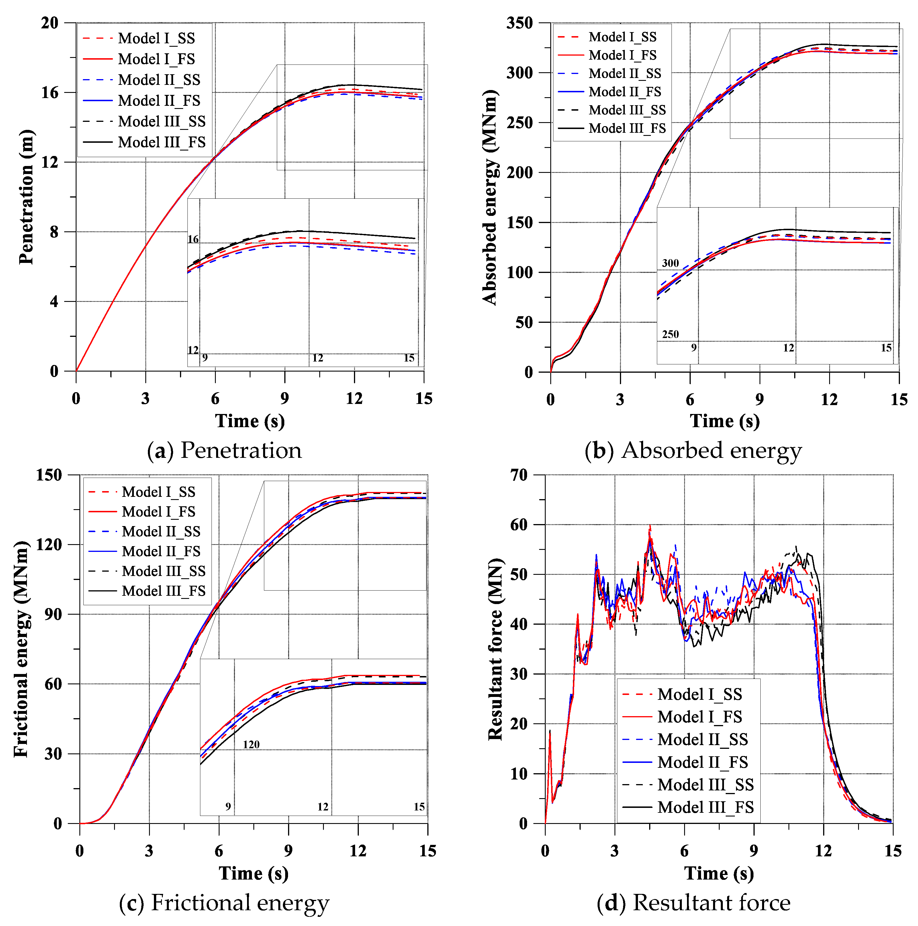
3. Effect of Boundary Conditions and Extent of Analysis
- Model I: 3 cargo holds (cargo No. 2–No.4);
- Model II: 1/2 + 1 + 1/2 cargo holds (half of cargo No. 2 + cargo No. 3 + half of cargo No. 4);
- Model III: 1 cargo hold (cargo No. 3).
- Simply supported (SS): dx, dy, and dz are fixed at the left end, and dy and dz are fixed at the right end. The rotational displacements are acceptable;
- Fixed supported (FS): All the translational and rotational displacements are fixed at both ends.
4. Case Study
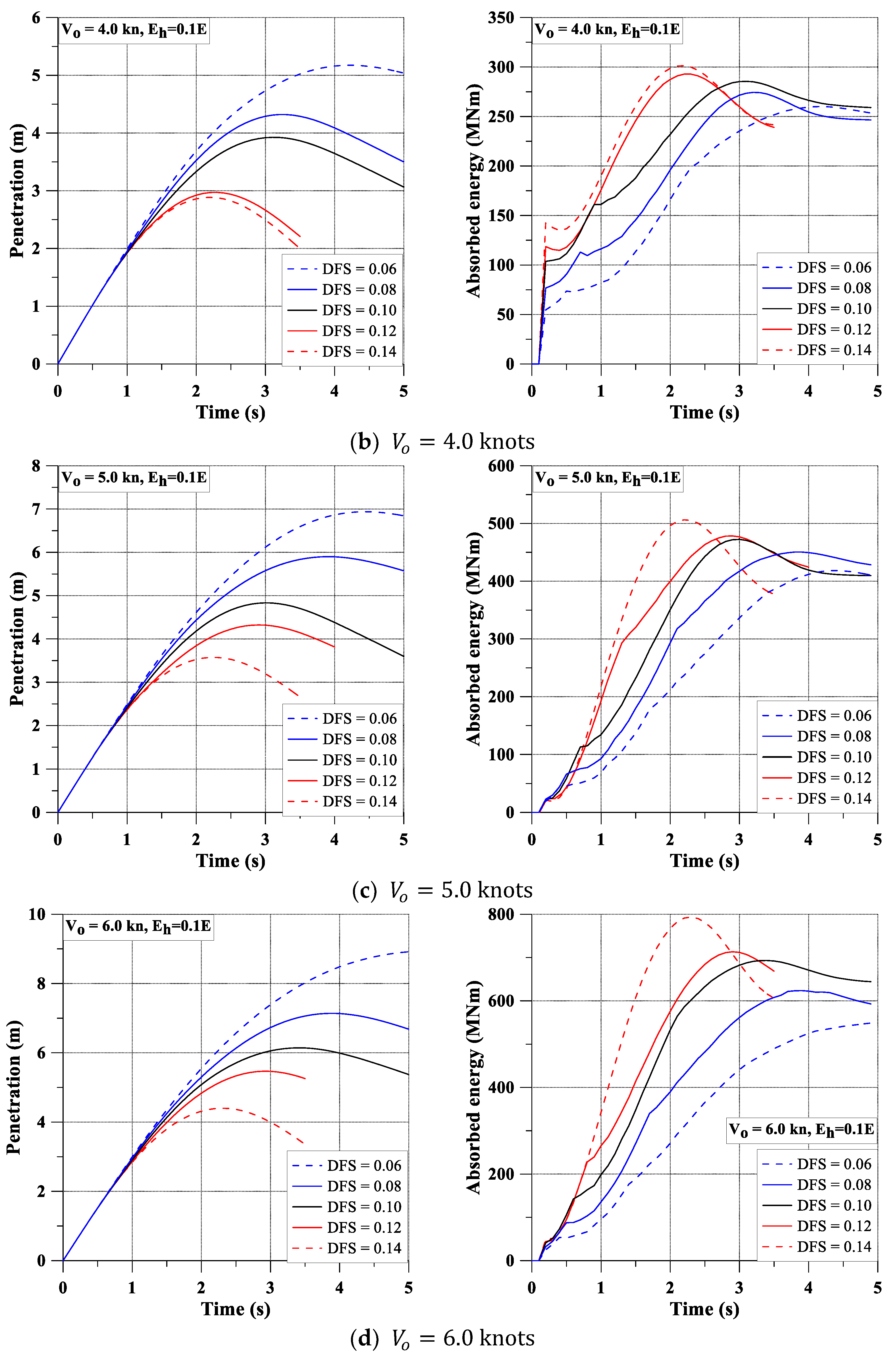
- Dynamic fracture strain, (-): 0.06, 0.08, 0.1 (Ref.), 0.12, 0.14;
- Initial impact speed, (knots): 2.5, 4, 5 (Ref.), 6, 7.5;
- Hardening tangent moduli (MPa): 0.0, 20580.
5. Results of Analysis
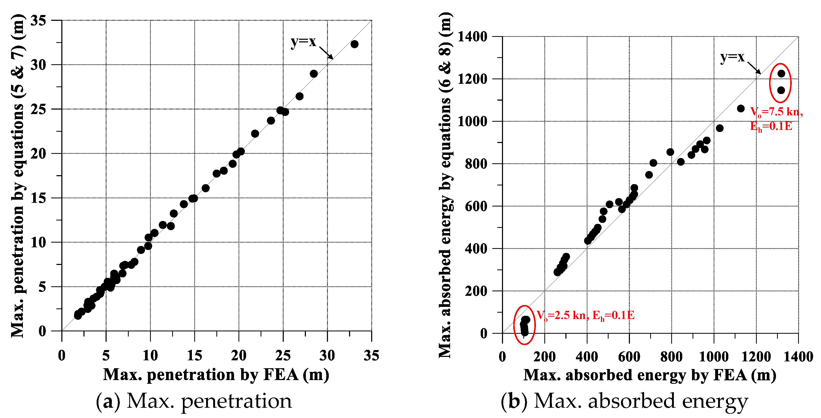
6. Development of an Empirical Formula
7. Application to Practical Exercise
8. Conclusions
- As the dynamic fracture strain increases, the penetration becomes shorter, but the amount of absorbed energy increases.
- When the structure is tougher (larger dynamic fracture strain), the energy consumption becomes faster.
- The effect of the dynamic fracture strain is minor under lower impact velocity when the hardening effect is not considered.
- The structure considering the hardening effect partially recovers owing to the elasticity. More structural members are affected by the impact load than in the results without the tangent moduli.
- The hardening effect is remarkable. The effect leads to smaller penetration and higher absorbed energy owing to the energy consumption by the structures around the damaged area. The effect results in widely distributed plastic strain.
- The tangent moduli have more of an impact on the responses when a relatively larger dynamic fracture strain is adopted.
- Maximum damage determined by the developed formula was in a good agreement with the FEA. It might be helpful to provide the upper and lower bounds of damage when considering various dynamic fracture strains for double sided oil tankers. However, it is recommended to use the formula for 4.0–6.0 knots of velocity when the hardening effect is considered.
Author Contributions
Funding
Institutional Review Board Statement
Informed Consent Statement
Data Availability Statement
Conflicts of Interest
References
- EMSA. Annual Overview of Marine Casualties and Incidents 2021; European Maritime Safety Agency: Lisbon, Portugal, 2021. [Google Scholar]
- Goerlandt, F.; Kujala, P. Modeling of Ship Collision Probability using Dynamic Traffic Simulation. Reliab. Risk Saf. 2010, 10, 440–447. [Google Scholar]
- Goerlandt, F.; Kujala, P. Traffic Simulation based Ship Collision Probability Modeling. Reliab. Eng. Syst. Saf. 2011, 96, 91–107. [Google Scholar] [CrossRef]
- Paik, J.K.; Kim, S.J.; Ko, Y.G.; Youssef, S.A.M. Collision Risk Assessment of a VLCC Class Tanker. In Proceedings of the Society of Naval Architects and Marine Engineers Maritime Convention, Houston, TX, USA, 23–28 October 2017. [Google Scholar]
- Kim, S.J.; Seo, J.K.; Ma, K.Y.; Park, J.S. Methodology for Collision-frequency Analysis of Wind-turbine Installation vessels. Ships Offshore Struct. 2021, 16, 423–439. [Google Scholar] [CrossRef]
- Namgung, H.; Kim, J.S. Regional Collision Risk Prediction System at a Collision Area Considering Spatial Pattern. J. Mar. Sci. Eng. 2021, 9, 1365. [Google Scholar] [CrossRef]
- Hong, L.; Amdahl, J. Plastic Mechanism Analysis of the Resistance of Ship Longitudinal Girders in Grounding and Collision. Ships Offshore Struct. 2008, 3, 159–171. [Google Scholar] [CrossRef]
- Liu, B.; Villavicencio, R.; Soares, C.G. Simplified Analytical Method to Evaluate Tanker Side Panels during Minor Collision Incidents. Int. J. Impact Eng. 2015, 78, 20–33. [Google Scholar] [CrossRef]
- Zeng, J.; Hu, Z.; Chen, G. A Steady-state Plate Tearing Model for Ship Grounding over a Cone-shaped Rock. Ships Offshore Struct. 2016, 11, 245–257. [Google Scholar] [CrossRef]
- Ehlers, S.; Tabri, K.; Romanoff, J.; Varsta, P. Numerical and Experimental Investigation on the Collision Resistance of the X-core Structure. Ships Offshore Struct. 2010, 7, 21–29. [Google Scholar] [CrossRef]
- Pedersen, T.P.; Zhang, S. Absorbed Energy in Ship Collisions and Groundings: Revising Minorsky’s Empirical Method. J. Ship Res. 2000, 44, 140–154. [Google Scholar] [CrossRef]
- Pedersen, T.P.; Zhang, S. Effect of Ship Structure and Size on Grounding and Collision Damage Distributions. Ocean Eng. 2000, 27, 1161–1179. [Google Scholar] [CrossRef]
- Paik, J.K.; Seo, J.K. A Method for Progressive Structural Crachworthiness Analysis under Collision and Grounding. Thin-Walled Struct. 2007, 45, 15–23. [Google Scholar] [CrossRef]
- Glykas, J.A.; Das, K.P. Energy Conservation during Grounding with Rigid Slopes. Ocean Eng. 2001, 28, 397–415. [Google Scholar] [CrossRef]
- Zhang, A.; Suzuki, K. Dynamic FE Simulations of the Effect of Selected Parameters on Grounding Test Results of Bottom Structures. Ships Offshore Struct. 2006, 1, 117–125. [Google Scholar] [CrossRef]
- Haris, S.; Amdahl, J. Crushing Resistance of a Cruciform and its Application to Ship Collision and Grounding. Ships Offshore Struct. 2012, 7, 185–195. [Google Scholar] [CrossRef]
- Nguyen, T.H.; Garré, L.; Amdahl, J.; Leira, B.J. Benchmark Study on the Assessment of Ship Damage Conditions during Stranding. Ships Offshore Struct. 2012, 7, 197–213. [Google Scholar] [CrossRef]
- Sohn, J.M.; Jung, D. Structural Assessment of a 500-Cbm Liquefied Natural Gas Bunker Ship during Bunkering and Marine Operation under Collision Accidents. Ships Offshore Struct. 2021. [Google Scholar] [CrossRef]
- Buldgen, L.; Le Sourne, H.; Rigo, P. A Simplified Analytical Method for Estimating the Crushing Resistance of an Inclined Ship Side. Mar. Struct. 2013, 33, 265–296. [Google Scholar] [CrossRef]
- Ferry, M.; Le Sourne, H.; Besnier, F. MCOL Theoretical Manual; Principia Marine: Nantes, France, 2002. [Google Scholar]
- Kim, S.J.; Kõrgersaar, M.; Ahmadi, N.; Taimuri, G.; Kujala, P.; Hirdaris, S. The Influence of Fluid Structure Interaction Modelling on the Dynamic Response of Ships Subject to Collision and Grounding. Mar. Struct. 2021, 75, 102875. [Google Scholar] [CrossRef]
- Kim, S.J.; Taimuri, G.; Kujala, P.; Conti, F.; Le Sourne, H.; Pineau, J.P.; Looten, T.; Bae, H.; Mujeeb-Ahmed, M.P.; Vassalos, D.; et al. Comparison of Numerical Approaches for Structural Response Analysis of Passenger Ships in Collisions and Groundings. Mar. Struct. 2022, 81, 103125. [Google Scholar] [CrossRef]
- Kim, S.J.; Sohn, J.M.; Kujala, P.; Hirdaris, S. A Simplifed Fluid Structure Interaction Model for the Assessment of Ship Hard Grouding. J. Mar. Sci. Technol. 2022, 27, 695–711. [Google Scholar] [CrossRef]
- Lehmann, E.; Egge, E.D.; Sharrer, M.; Zhang, L. Calculation of Collision with the Aid of Linear FE models. In Proceedings of the International Conference on Practical Design of Ships and Mobile Units, Shanghai, China, 16–21 September 2001. [Google Scholar]
- Ko, Y.G.; Kim, S.J.; Sohn, J.M.; Paik, J.K. A Practical Method to Determine the Dynamic Fracture Strain for the Nonlinear Finite Element Analysis of Structural Crashworthiness in Ship-ship Collisions. Ships Offshore Struct. 2018, 13, 412–422. [Google Scholar] [CrossRef] [Green Version]
- ANSYS/LS-DYNA. User’s Manual for ANSYS/LS-DYNA, Version 2020R1; ANSYS Inc.: Canonsburg, PA, USA, 2020. [Google Scholar]
- Jones, N. Structural Impact, 2nd ed.; Cambridge University Press: Cambridge, UK, 2012. [Google Scholar]


| Length overall (m) | 318.2 |
| Breadth (m) | 60.0 |
| Depth (m) | 30.0 |
| Design draft (m) | 21.6 |
| Deadweight (ton) | 320,000 |
| Displacement (ton) | 364,000 |
| Block coefficient | 0.81 |
(kg/m3) | (MPa) | (GPa) | Cowper–Symonds Coefficient | |
|---|---|---|---|---|
| C | q | |||
| 7850 | 235 | 205.8 | 40.4 | 5 |
| Extent of Analysis | Boundary Conditions | Max. Penetration (m) | Max. Absorbed Energy (MNm) | Max. Frictional Energy (MNm) |
|---|---|---|---|---|
| Model I | SS | 16.19 | 324.38 | 140.18 |
| FS | 16.02 | 321.52 | 142.40 | |
| Model II | SS | 15.89 | 323.88 | 140.14 |
| FS | 16.01 | 321.24 | 140.27 | |
| Model III | SS | 16.43 | 324.83 | 142.08 |
| FS | 16.42 | 328.42 | 139.78 |
| DFS (-) | (knots) | Max. Pen. (m) | Max. Ab. E. (MNm) | DFS (-) | (knots) | Max. Pen. (m) | Max. Ab. E. (MNm) |
|---|---|---|---|---|---|---|---|
| 0.06 | 2.5 | 7.839 | 105.925 | 0.06 | 2.5 | 3.345 | 100.351 |
| 0.08 | 6.846 | 107.981 | 0.08 | 2.927 | 102.705 | ||
| 0.10 | 6.186 | 111.400 | 0.10 | 2.226 | 104.330 | ||
| 0.12 | 5.599 | 112.688 | 0.12 | 1.856 | 105.362 | ||
| 0.14 | 5.500 | 113.601 | 0.14 | 1.822 | 108.510 | ||
| 0.06 | 4 | 14.746 | 259.824 | 0.06 | 4 | 6.938 | 418.390 |
| 0.08 | 12.641 | 271.570 | 0.08 | 5.900 | 450.500 | ||
| 0.10 | 11.403 | 279.929 | 0.10 | 4.833 | 472.400 | ||
| 0.12 | 10.469 | 284.048 | 0.12 | 4.323 | 478.398 | ||
| 0.14 | 9.803 | 289.628 | 0.14 | 3.572 | 506.303 | ||
| 0.06 | 5 | 19.725 | 403.621 | 0.06 | 5 | 5.174 | 260.060 |
| 0.08 | 17.485 | 418.423 | 0.08 | 4.320 | 274.409 | ||
| 0.10 | 16.244 | 427.263 | 0.10 | 3.925 | 285.528 | ||
| 0.12 | 14.935 | 436.943 | 0.12 | 2.972 | 292.830 | ||
| 0.14 | 13.780 | 445.212 | 0.14 | 2.886 | 301.330 | ||
| 0.06 | 6 | 24.683 | 564.638 | 0.06 | 6 | 8.939 | 550.346 |
| 0.08 | 21.823 | 586.331 | 0.08 | 7.139 | 623.568 | ||
| 0.10 | 20.220 | 600.979 | 0.10 | 6.144 | 693.100 | ||
| 0.12 | 19.294 | 615.532 | 0.12 | 5.468 | 713.298 | ||
| 0.14 | 18.294 | 622.905 | 0.14 | 4.400 | 793.600 | ||
| 0.06 | 7.5 | 33.066 | 843.162 | 0.06 | 7.5 | 12.308 | 956.280 |
| 0.08 | 28.461 | 893.403 | 0.08 | 9.747 | 1027.400 | ||
| 0.10 | 26.858 | 912.507 | 0.10 | 8.202 | 1126.999 | ||
| 0.12 | 25.221 | 934.599 | 0.12 | 5.908 | 1317.301 | ||
| 0.14 | 23.619 | 965.816 | 0.14 | 5.743 | 1318.601 | ||
| (knots) | ||||||
| 2.5 | 20.463 | −5.917 | 0.764 | −1.846 | 0.604 | 0.218 |
| 4 | 34.979 | −10.708 | 1.420 | −6.568 | 2.229 | 0.500 |
| 5 | 23.126 | −9.070 | 1.669 | −5.110 | 2.212 | 0.832 |
| 6 | 48.333 | −14.378 | 2.200 | −12.010 | 4.107 | 1.119 |
| 7.5 | 65.652 | −19.944 | 2.975 | −14.653 | 6.283 | 1.660 |
| 2.5 | 40.629 | −12.386 | 1.304 | 0.376 | 0.126 | 0.204 |
| 4 | 36.161 | −13.361 | 1.743 | −5.866 | 2.242 | 0.438 |
| 5 | 41.807 | −16.957 | 2.302 | −9.190 | 3.994 | 0.685 |
| 6 | 65.938 | −24.307 | 3.046 | −13.296 | 8.758 | 0.696 |
| 7.5 | 149.380 | −47.430 | 4.864 | −18.498 | 14.438 | 1.189 |
| Collision Scenario | Max. Structural Response | ||||
|---|---|---|---|---|---|
(knots) | Collision Angle (°) | (-) | (MPa) | Penetration (m) | Absorbed Energy (MNm) |
| 5 | 90 | 0.1 | 0.0E | 10.43 | 32.93 |
Publisher’s Note: MDPI stays neutral with regard to jurisdictional claims in published maps and institutional affiliations. |
© 2022 by the authors. Licensee MDPI, Basel, Switzerland. This article is an open access article distributed under the terms and conditions of the Creative Commons Attribution (CC BY) license (https://creativecommons.org/licenses/by/4.0/).
Share and Cite
Kim, S.J.; Sohn, J.M. The Effect of Dynamic Fracture Strain on the Structural Response of Ships in Collisions. J. Mar. Sci. Eng. 2022, 10, 1674. https://doi.org/10.3390/jmse10111674
Kim SJ, Sohn JM. The Effect of Dynamic Fracture Strain on the Structural Response of Ships in Collisions. Journal of Marine Science and Engineering. 2022; 10(11):1674. https://doi.org/10.3390/jmse10111674
Chicago/Turabian StyleKim, Sang Jin, and Jung Min Sohn. 2022. "The Effect of Dynamic Fracture Strain on the Structural Response of Ships in Collisions" Journal of Marine Science and Engineering 10, no. 11: 1674. https://doi.org/10.3390/jmse10111674