
A Simplified Calculation Method for Cyclic Response of Laterally Loaded Piles Based on Strain Wedge Model in Soft Clay

 ,
, 
Abstract
:1. Introduction
2. Large-Diameter Single Pile Cyclic Response Calculation Model
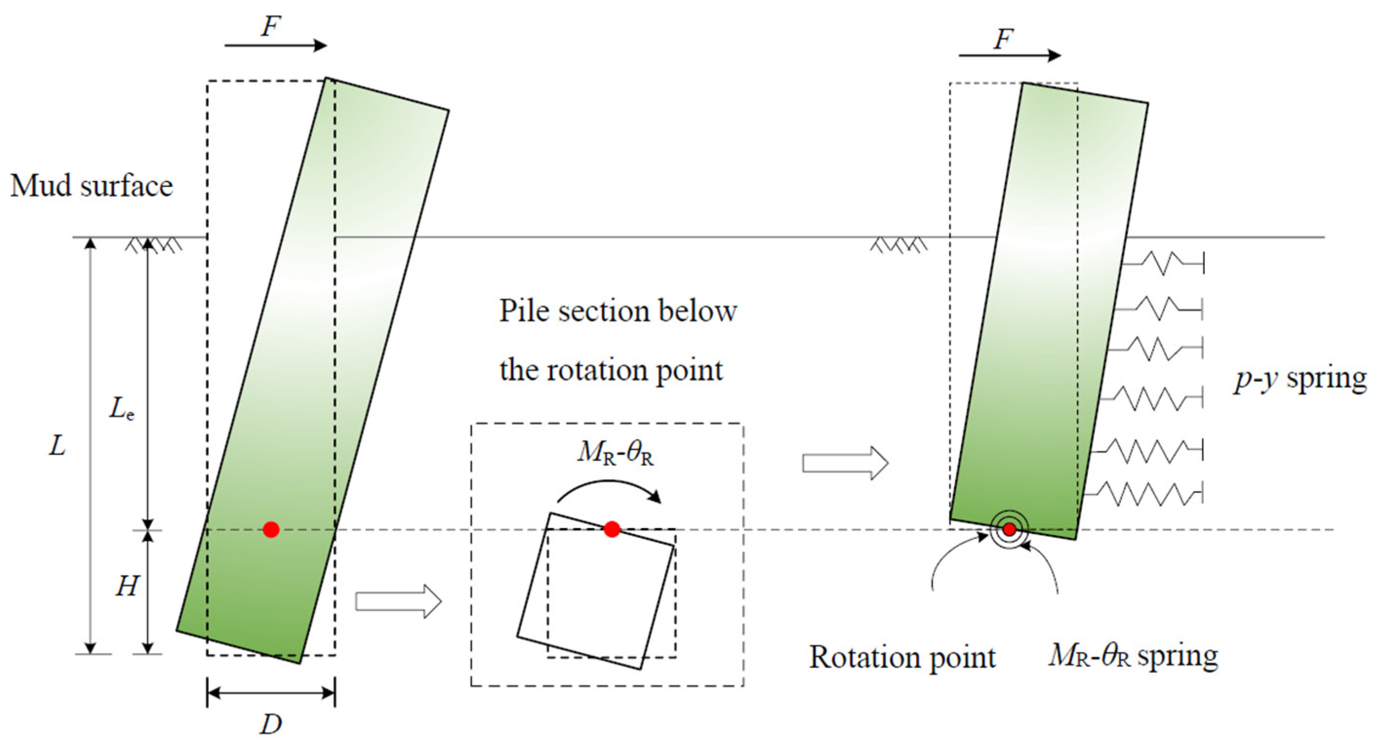
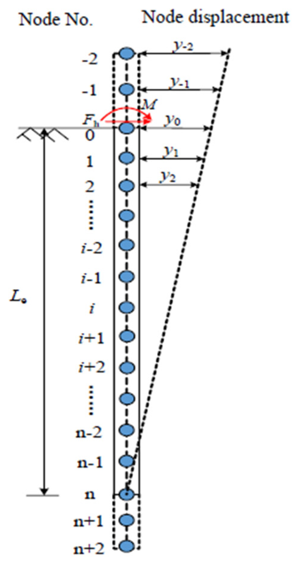
2.1. Simplified Calculation Model
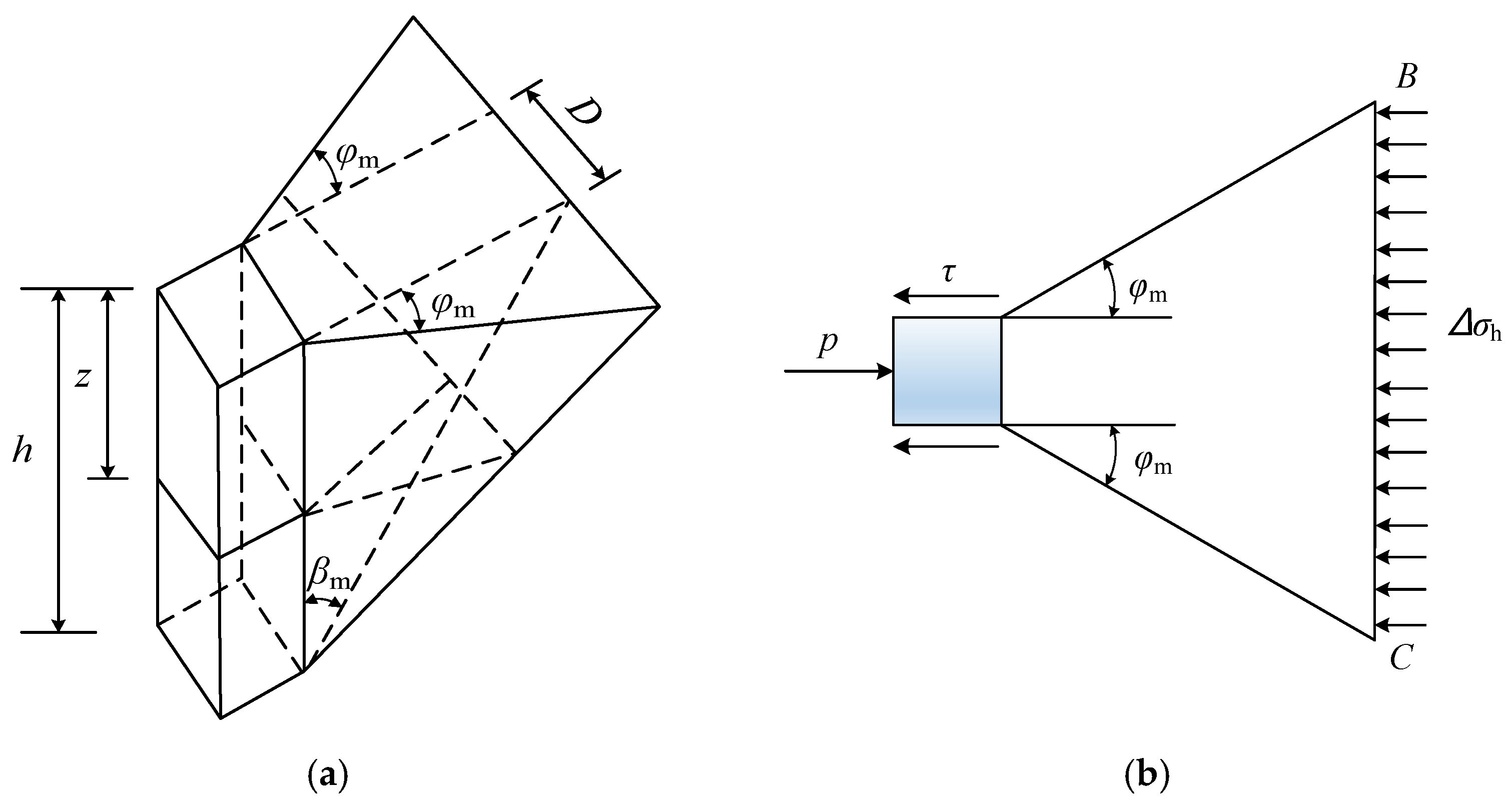
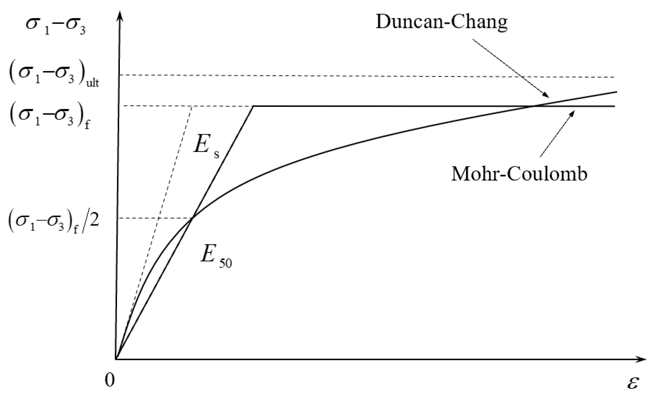
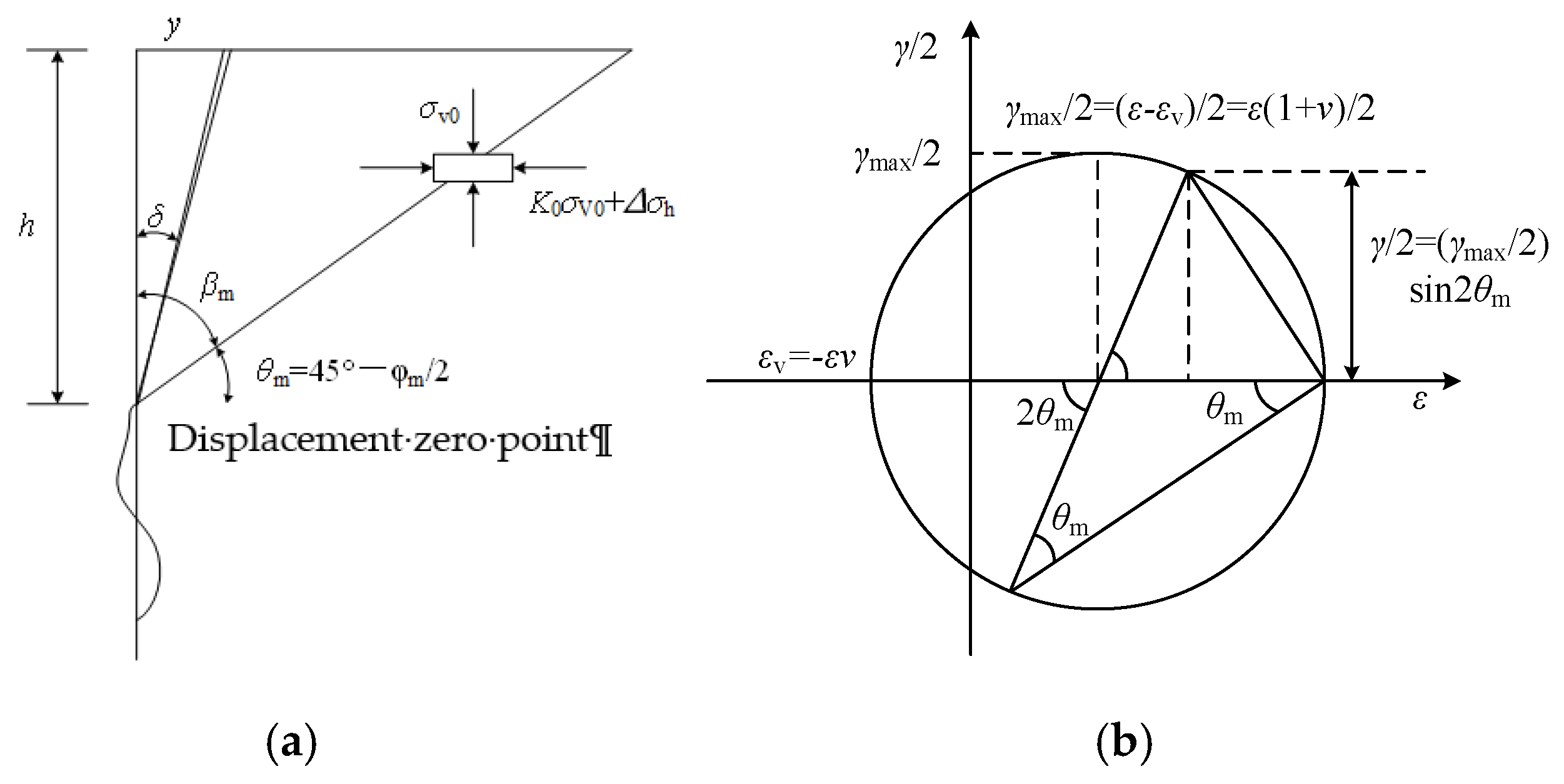
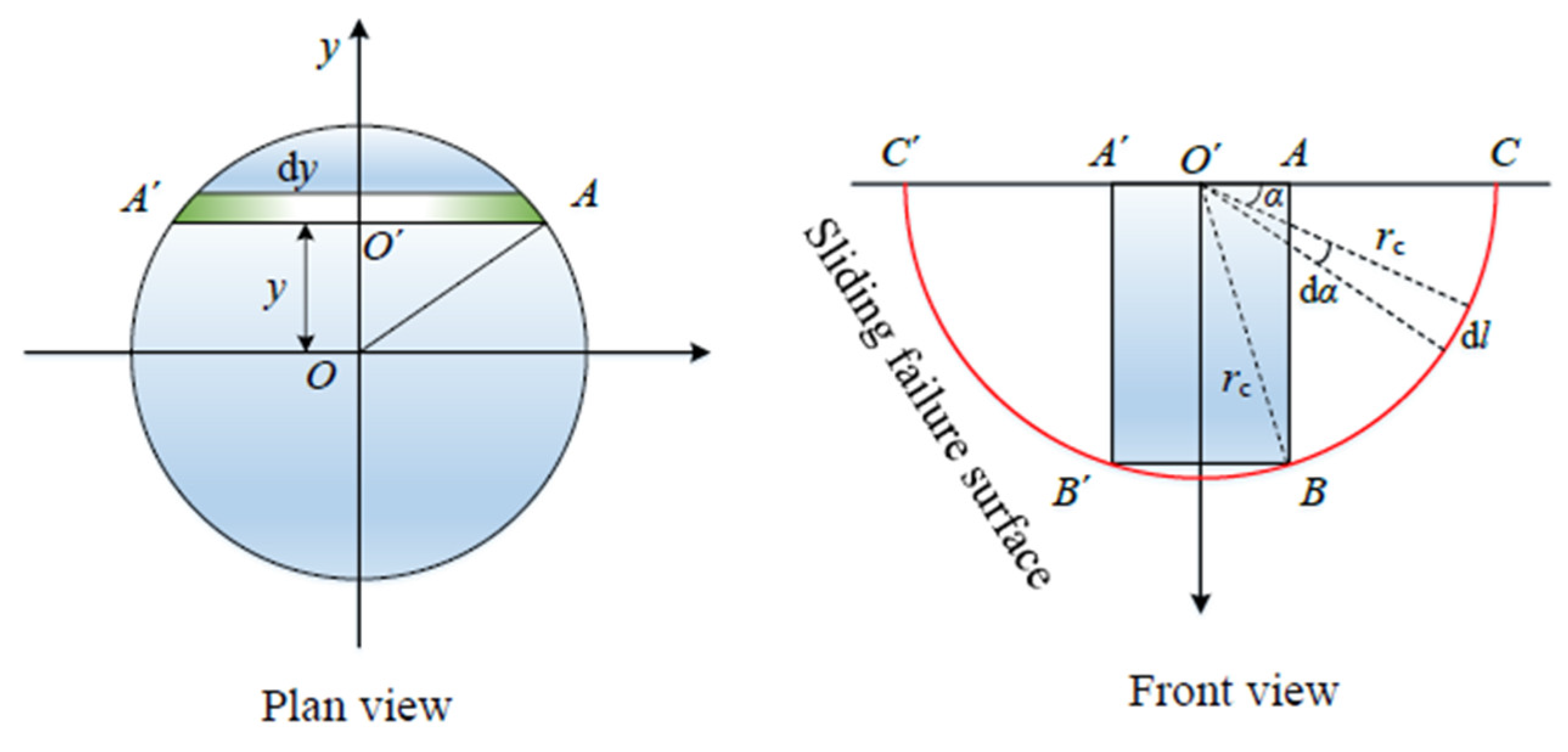
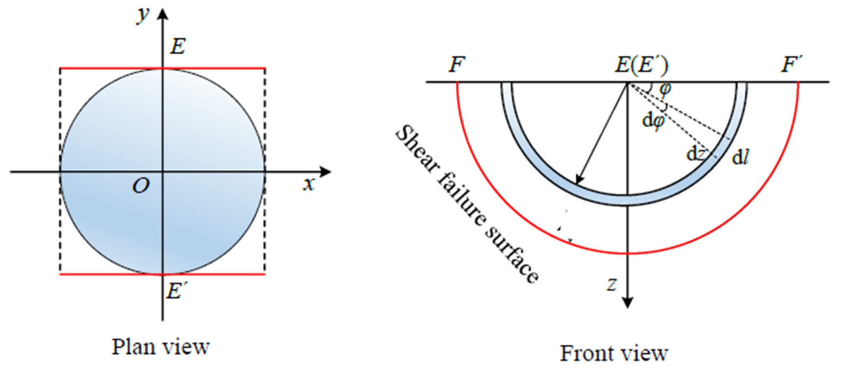
2.2. Strain Wedge Model
2.3. MR–θR Model
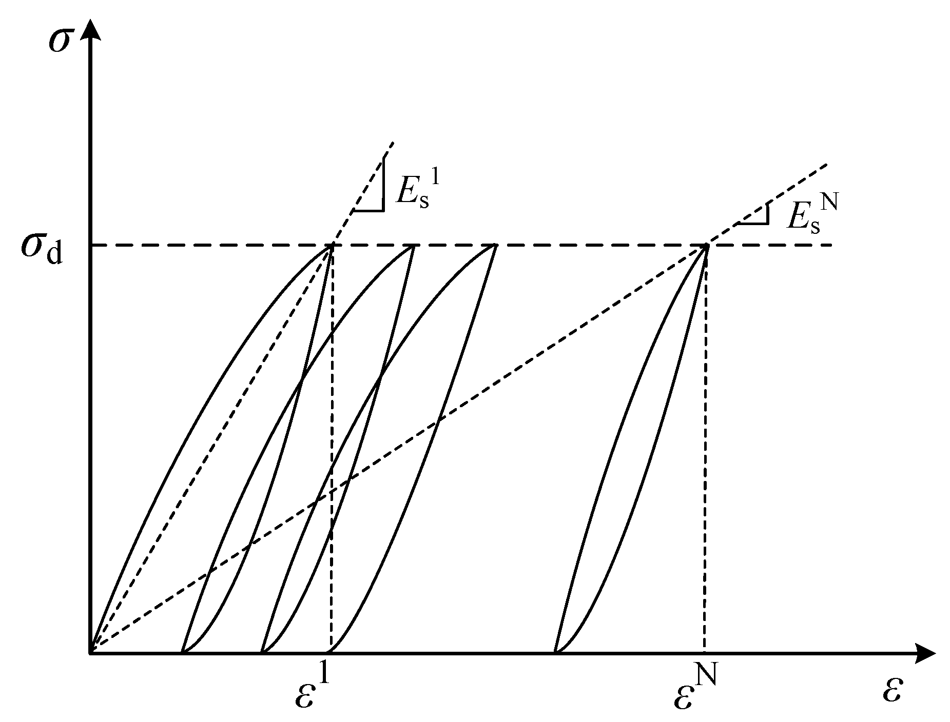
2.4. Stiffness Attenuation Model
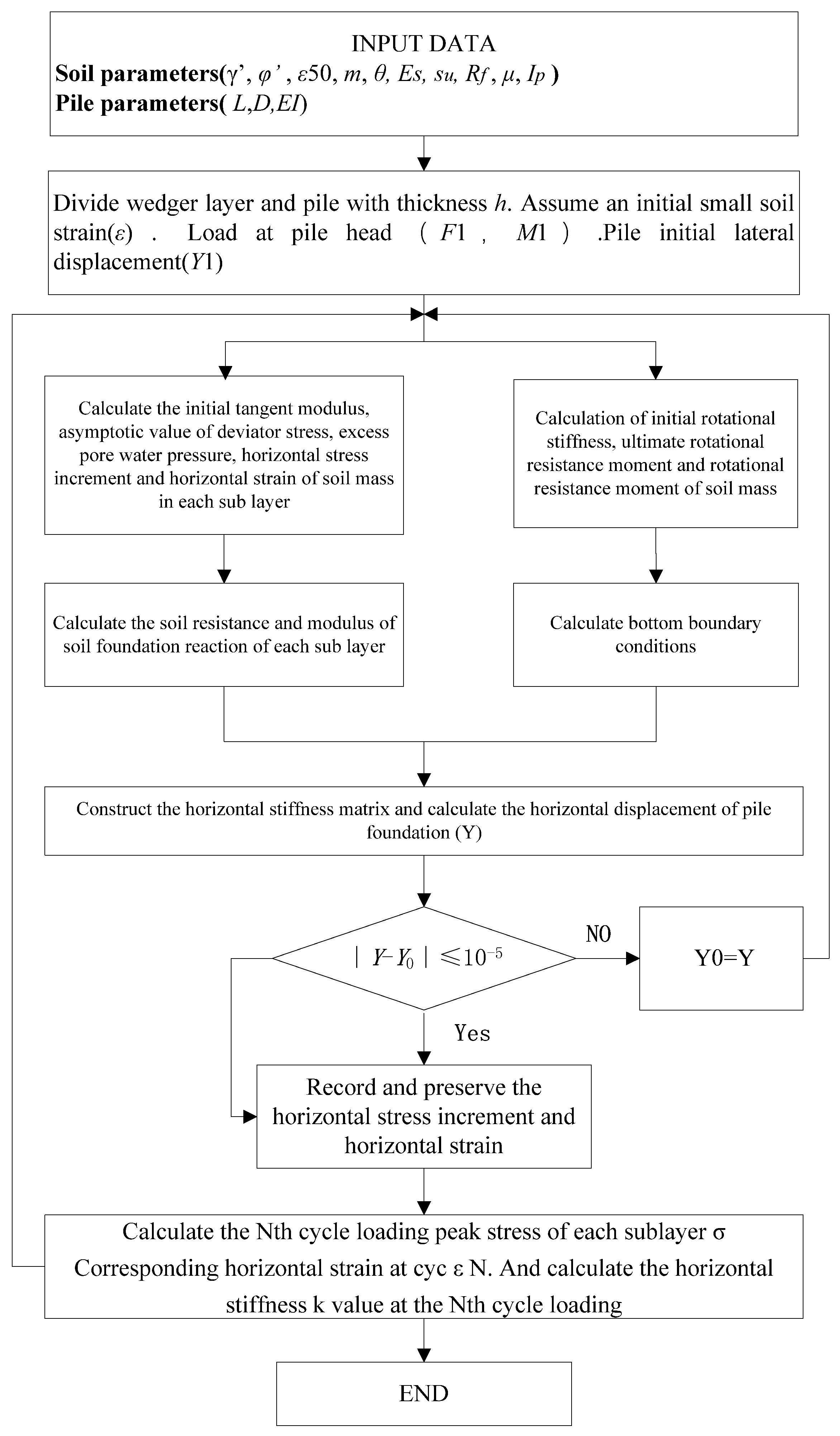
2.5. Calculation Method and Program Implementation
3. Method Validation
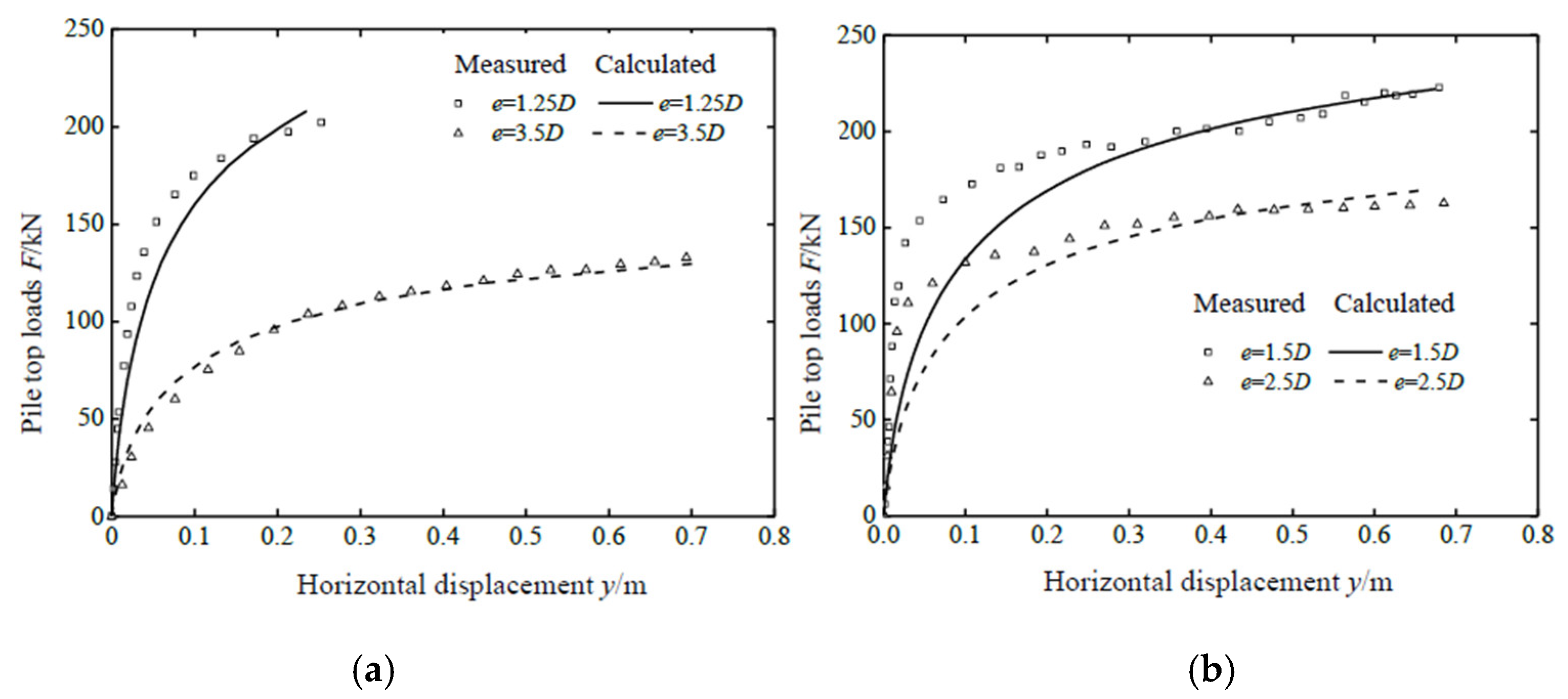
3.1. Case 1
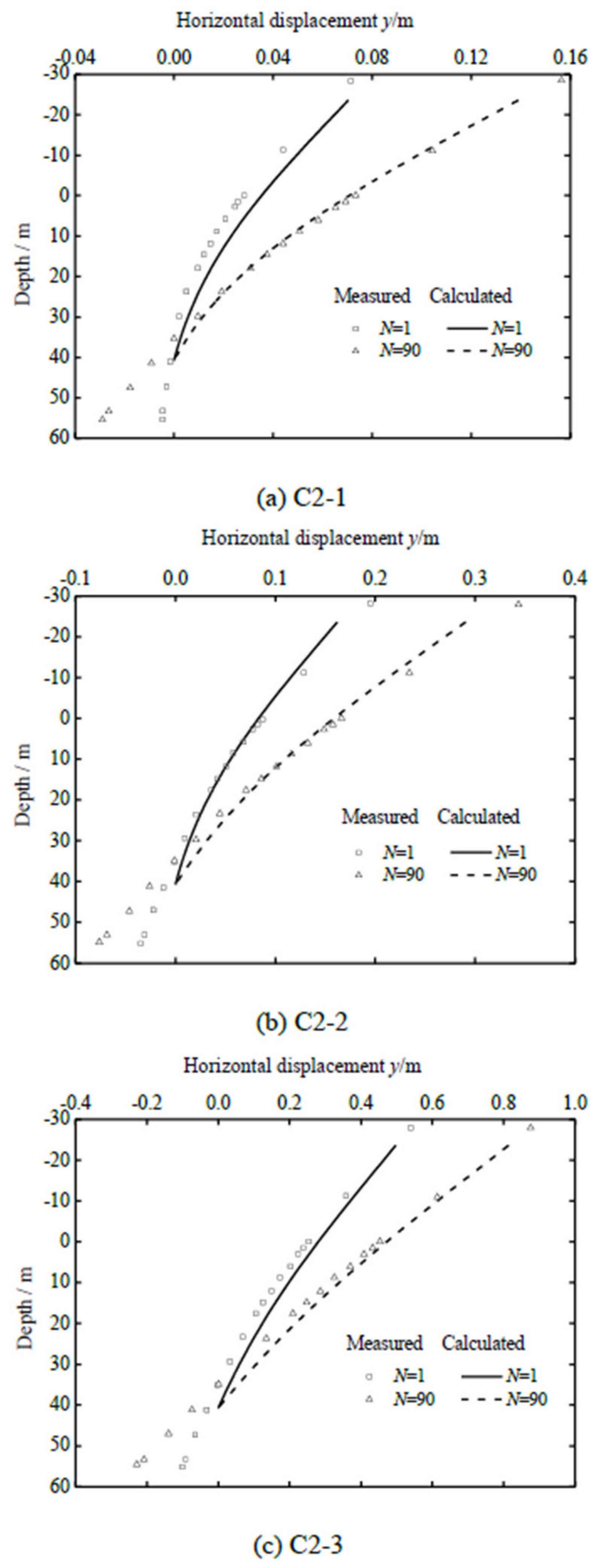
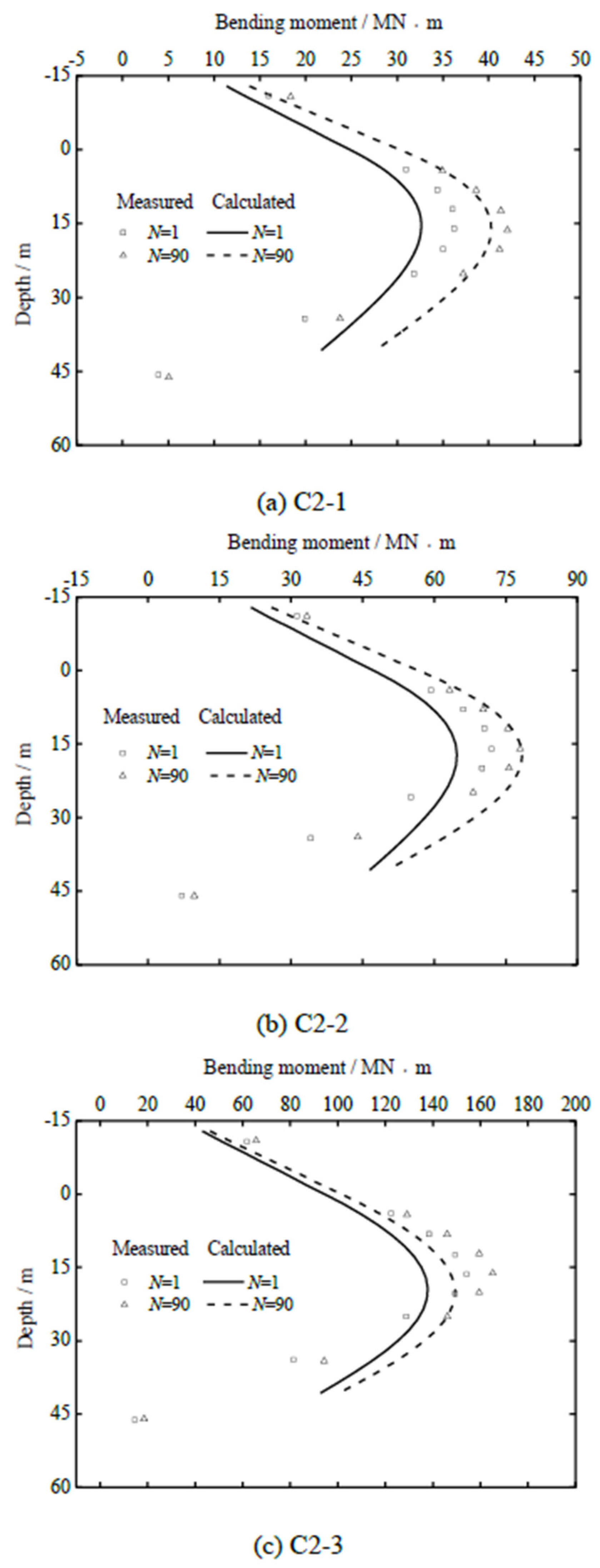
3.2. Case 2
4. Conclusions
Author Contributions
Funding
Institutional Review Board Statement
Informed Consent Statement
Data Availability Statement
Acknowledgments
Conflicts of Interest
References
- Jeanjean, P. Re—assessment of p–y curves for soft clays from centrifuge testing and finite element modeling. In Proceedings of the Offshore Technology Conference, Paper No. OTC 20158, Houston, TX, USA, 4–7 May 2009; pp. 1–23. [Google Scholar]
- Kodikara, J.; Haque, A.; Lee, K.Y. Theoretical p-y Curves for Laterally Loaded Single Piles in Undrained Clay Using Bezier Curves. J. Geotech. Geoenviron. Eng. 2010, 136, 265–268. [Google Scholar] [CrossRef]
- Reese, L.C.; Welch, R.C. Lateral Loading of Deep Foundations in Stiff Clay. J. Geotech. Eng. Div. 1975, 101, 633–649. [Google Scholar] [CrossRef]
- Sullivan, W.R.; Reese, L.C.; Fenske, C.W. Unified Method for Analysis of Laterally Loaded Piles in Clay. In Numerical Methods in Offshore Piling; Institution of Civil Engineers: London, UK, 1980; pp. 135–146. [Google Scholar]
- Dunnavant, T.W.; O’Neill, M.W. Experimental p–y model for submerged stiff clay. J. Geotech. Eng. 1989, 115, 95–114. [Google Scholar] [CrossRef]
- Georgiadis, M.; Anagnostopoulos, C.; Saflekou, S. Centrifugal testing of laterally loaded piles in sand. Can. Geotech. J. 1992, 29, 208–216. [Google Scholar] [CrossRef]
- API. Geotechnical and Foundation Design Considerations, ANSI/API Recommended Practice 2 GEO, 1st ed.; API: Washington, DC, USA, 2011. [Google Scholar]
- DNV. Design of Offshore Wind Turbine Structures. In Recommended Practice DNV–RP–H103; Det Norske Veritas: Baerum, Norway, 2011. [Google Scholar]
- American Petrolem Institute. Recommended Practice for Planning Designing and Constructing Fixed Offshore Platforms-Working Stress Design; American Petroleum Institute Publishing Services: Washington, DC, USA, 2005. [Google Scholar]
- Byrne, B.W.; Houlsby, G.T.; Burd, H.J.; Gavin, K.G. PISA design model for monopiles for offshore wind turbines: Application to a stiff glacial clay till. Géotechnique 2020, 70, 1030–1047. [Google Scholar] [CrossRef]
- Fu, D.F.; Zhang, Y.H.; Aamodt, K.K.; Yan, Y. A multi-spring model for monopiles analysis in soft clay. Mar. Struct. 2020, 72, 102768. [Google Scholar] [CrossRef]
- Wang, L.Z.; Lai, Y.Q.; Hong, Y.; Maín, D. A unified lateral soil reaction model for monopiles in soft clay considering various lengt-to-diameter (L/D) ratios. Ocean. Eng. 2020, 212, 107492. [Google Scholar] [CrossRef]
- Norris, G.M. Theoretically based BEF laterally loaded pile analysis. In Proceedings of the 3rd International Conference on Numerical Methods in Offshore Piling, Nantes, France, 21–22 May 1986; pp. 361–386. [Google Scholar]
- Ashour, M.; Norris, G.; Pilling, P. Lateral loading of a pile in layered soil using the strain wedge model. J. Geotech. Geoenviron. Eng. 1998, 124, 303–315. [Google Scholar] [CrossRef]
- Ashour, M.; Norris, G. Modeling lateral soil–pile response based on soil–pile interaction. J. Geotech. Geoenviron. Eng. 2000, 126, 420–428. [Google Scholar] [CrossRef]
- Xu, L.; Cai, F.; Wang, G.X.; Ugai, K. Nonlinear analysis of laterally loaded single piles in sand using modified strain wedge model. Comput. Geotech. 2013, 51, 60–71. [Google Scholar] [CrossRef]
- Duncan, J.M.; Chang, C.Y. Nonlinear analysis of stress and strain in soils. J. Soil. Mech. Found. Div. 1970, 96, 1629–1653. [Google Scholar] [CrossRef]
- Yang, X.; Zhang, C.; Huang, M.S.; Yuan, J.Y. Lateral loading of a pile using strain wedge model and its application under scouring. Mar. Geo. Geotech. 2017, 6, 340–350. [Google Scholar] [CrossRef]
- Peng, W.; Zhao, M.; Xiao, Y.; Yang, C.W.; Zhao, H. Analysis of laterally loaded piles in sloping ground using a modified strain wedge model. Comput. Geotech. 2019, 107, 163–175. [Google Scholar] [CrossRef]
- Zhu, W.B.; Dai, G.L.; Wang, B.C.; Gong, W.M.; Sun, J.; Hu, H. Study on cyclic characteristics and equivalent cyclic creep model of the soft clay at the bottom of suction caisson foundation. Rock Soil Mech. 2022, 43, 466–478. [Google Scholar]
- Yi, B.; Lw, B.; Yz, A.; Yi, H.B. Site-specific soil model for monopiles in soft clay based on laboratory element stress-strain curves. Ocean. Enineering 2021, 220, 108437. [Google Scholar]
- Brinkgreve, R.B.J. Plaxis User’s Manual-Version 8; Balkema: Rotterdam, The Netherlands, 2002. [Google Scholar]
- Idriss, I.M.; Singh, R.D.; Dobry, R. Nonlinear behavior of soft clays during cyclic loading. J. Geotech. Eng. Div. 1978, 104, 1427–1447. [Google Scholar] [CrossRef]
- Yasuhara, K.; Hyde, A.F.L.; Toyota, N. Cyclic stiffness of plastic silt with an initial drained shear stress. In Pre-Failure Deformation of Geoterials; Thomas Telford Ltd.: London, UK, 1998; pp. 373–382. [Google Scholar]
- Li, S.; Huang, M.S. Undrained long-term cyclic degradation characteristics of offshore soft clay. In Soil Dynamics and Earthquake Engineering; ASCE: Reston, VA, USA, 2010; pp. 263–271. [Google Scholar]
- Murali, M.; Hrajales-Saavedra, F.J.; Beemer, R.D.; Aubeny, C.P.; Biscontin, G. Capacity of short piles and casissons in soft clay from geotechnical centrifuge tests. J. Geotech. Geoenviron. Eng. 2019, 145, 04019079. [Google Scholar] [CrossRef]
- Yang, Q.J.; Gao, Y.F.; Kong, D.Q.; Zhu, B. Centrifuge modelling of lateral loading behavior of a “semi-rigid” monopile in soft clay. Mar. Georesources Geotechnol. 2019, 37, 1205–1216. [Google Scholar] [CrossRef]


Publisher’s Note: MDPI stays neutral with regard to jurisdictional claims in published maps and institutional affiliations. |
© 2022 by the authors. Licensee MDPI, Basel, Switzerland. This article is an open access article distributed under the terms and conditions of the Creative Commons Attribution (CC BY) license (https://creativecommons.org/licenses/by/4.0/).
Share and Cite
Liu, X.; Yao, Z.; Zhu, W.; Zhang, Y.; Yan, S.; Guo, X.; Dai, G. A Simplified Calculation Method for Cyclic Response of Laterally Loaded Piles Based on Strain Wedge Model in Soft Clay. J. Mar. Sci. Eng. 2022, 10, 1632. https://doi.org/10.3390/jmse10111632
Liu X, Yao Z, Zhu W, Zhang Y, Yan S, Guo X, Dai G. A Simplified Calculation Method for Cyclic Response of Laterally Loaded Piles Based on Strain Wedge Model in Soft Clay. Journal of Marine Science and Engineering. 2022; 10(11):1632. https://doi.org/10.3390/jmse10111632
Chicago/Turabian StyleLiu, Xin, Zhongyuan Yao, Wenbo Zhu, Yu Zhang, Shu Yan, Xiaojiang Guo, and Guoliang Dai. 2022. "A Simplified Calculation Method for Cyclic Response of Laterally Loaded Piles Based on Strain Wedge Model in Soft Clay" Journal of Marine Science and Engineering 10, no. 11: 1632. https://doi.org/10.3390/jmse10111632