Finite-Time Extended State Observe Based Fault Tolerant Control for Autonomous Underwater Vehicle with Unknown Thruster Fault

Abstract

This paper investigates the problem of fault tolerant control (FTC) for autonomous underwater vehicles (AUVs) with multiple thrusters in the presence of current disturbances, thruster faults, and modelling uncertainty. This paper focuses on the problems of reducing the energy consumption caused by the chattering of control signals and improving the tracking accuracy of an AUV operating in deep-sea environments. In view of the problem of large energy consumption in some other methods, a fault tolerant control method for multiple-thruster AUVs based on a finite-time extended state observer (FTESO) is proposed. More specifically, a FTESO based on an integral sliding mode surface is designed to estimate the generalized uncertainty compounded using current disturbances, thruster faults, and modelling uncertainty. The fast finite-time uniformly ultimately bounded stability of the proposed FTESO is analyzed. Then, based on the estimated value of FTESO, an FTC method based on non-singular fast terminal sliding mode surfaces is developed for AUVs. The finite-time convergence of the closed-loop control system is proved theoretically. In this design, two different sliding mode surfaces are used to design FTESO and FTC, in order to avoid the appearance of singularities. Moreover, a parameter adjustment method is designed to improve tracking accuracy. Finally, comparative numerical simulations show that the proposed control scheme is effective at reducing energy consumption and improving tracking accuracy.

1. Introduction

Because of the great advantages in terms of operating automatically in the deep-sea environments, autonomous underwater vehicles (AUVs) equipped with multiple thrusters play an important role in many tasks, including the detection of marine resources, seafloor mapping, and crashed aircraft search [1,2,3]. As AUVs operate in the unknown and complicated deep-sea environment, safety is one of the important issues to be considered [4]. Fault tolerant control (FTC) is the key technology to ensure the safety of AUVs [5]. Thrusters are the main power consumers on an AUV, and they are also the components that experience the heaviest loading and are thus the most prone to faults [6]. The failure of a thruster directly affects the safety of an AUV operating in deep areas [7]. Therefore, fault tolerant control for AUV thrusters is one of the current research hotspots in this field [6]. This paper focuses on fully actuated AUVs. Fully actuated AUVs equipped with manipulators have unique capabilities to complete missions, such as grasping or cutting [8].

Nowadays, two main FTC methods exist, that is, passive fault tolerant control (PFTC) and active fault-tolerant control (AFTC) [9]. The former can deal with some classes of faults specified and considered during the controller design process, but the fault tolerant control performance is poor for faults that are not of the specified class. As for the AFTC, it has attracted much attention in the past decades because of its feasibility and effectiveness to deal with unknown faults [10].

In the field of AUVs, AFTC is mainly divided into two types: AFTC based on thrust reallocation, and adaptive FTC [11]. The former is based on the premise of known fault information. However, in a complex marine environment, the dynamic performance of an AUV varies with the environment and is disturbed by random currents, so it is difficult to obtain accurate fault diagnosis results sufficiently quickly to compensate for the fault. Thus, this method has limitations in AUV fault tolerant control [12]. The adaptive FTC approach treats faults as a generalized uncertainty and then uses adaptive strategies to estimate its upper bounds along with its disturbances [13]. It is also suitable for vehicles such as AUVs that move in complex environments [14]. Adaptive FTC has developed rapidly and achieved good research results in recent years [15,16]. For AUVs subject to ocean current disturbances and modelling uncertainty, researchers have investigated a virtual closed-loop adaptive FTC method, which avoids serious chattering phenomena in control outputs. Su et al. [17] proposed an event-triggered adaptive FTC scheme, which solves the trajectory tracking control problem for AUVs with actuator faults and model uncertainties.

In the fault-tolerant control of AUVs, there are problems with system dynamic model uncertainty and external disturbances [16]. The adaptive FTC method based on observer estimation is suitable for moving vehicles in complex environments. The observer has a good effect in dealing with nonlinear dynamics due to disturbances and faults [18,19], and the so-called extended state observer (ESO) has been considered as an effective way to actively compensate for uncertainty and disturbances [20,21]. The key idea of ESO is that system uncertainties and disturbances are considered as an added or extended state of the system, and then all the states including the extended one will be estimated accurately and quickly by the ESO.

In recent years, ESO has been effectively applied in many fields [22]. In [22], a nonsingular fast terminal sliding mode control (NFTSMC) based on a third-order fast finite-time extended state observer was proposed for the trajectory tracking of AUVs with various hydrodynamic uncertainties and external disturbances. Specifically, ref. [22] constructed the extended state variable according to the velocity information and constructed a third-order FFTESO to realize the finite-time estimation of the extended state variable. Another typical example is that Li proposed robust fault-tolerant control for a spacecraft system based on a finite-time ESO (FTESO) [23], where the FTESO and controller design shared a non-singular terminal sliding mode surface (NTSMS). The proposed control scheme was continuous with the property of restraining chattering. However, in the research on fault-tolerant control of fully actuated AUV thrusters based on the above methods [23], it was found that the control law derived theoretically from the AUV had singularities, and from the experimental results, the control output chattering was serious, which would lead to energy consumption increases.

Motivated by the mentioned-above discussion, this paper studies the FTC problem based on FTESO for a fully actuated AUV in the presence of current disturbances, thruster faults, and dynamic model uncertainty. In this paper, an improved FTC method based on FTESO is proposed, which aims to reduce the energy consumption caused by the chattering of the control signal under the premise of ensuring a high tracking accuracy. The main contributions of this paper are as follows.

(1) In a previous approach [23], the design of FTESO and the controller share an NTSMS, but this paper uses two sliding mode surfaces respectively for the FTESO and the controller. In the design of FTESO in this paper, the integral sliding mode surface (ISMS) was used to replace the NTSMS, so that the coefficient of the generalized uncertainty term after the derivation of the sliding mode surface was 1, that is, the generalized uncertainty term was directly used in the design of the control law. The estimated value of the uncertain item replaces the real value. This is different to the approach of [23], which requires the estimated value to remove the fractional power term of the velocity error to obtain the real value. In particular, when the velocity error term tends to zero, the method in this paper effectively suppresses the fluctuation of the generalized uncertainty term and avoids the appearance of singular points.

(2) To design an FTESO based on ISMS, this paper replaces NTSMS with a non-singular fast terminal sliding mode surface (NFTSMS) in the design of a fault-tolerant controller. That is, the generalized uncertainty term estimated by FTESO is applied to the newly designed NFTSMS to derive the control law. This avoids the pseudo-inverse term of the velocity error with the fractional power that appears in the control gain of the method in [23], thus, it can effectively suppress the chattering of the control variable, thereby reducing the energy consumption.

(3) The FTESO-based fault-tolerant control (FTESO − FTC) method proposed in this paper has a good effect in reducing energy consumption, but it has the problem of reducing the tracking accuracy. Therefore, this paper adds a parameter adjustment method (PAM).

The remainder of this paper is structured as follows. Section 2 presents a mathematical model, notations, and some useful lemmas. In Section 3, the ISMS-based FTESO is designed and analyzed. The NFTSMS-based FTC design and convergence analysis and the PAM for AUV thruster control are described in Section 4. In Section 5, comparative simulations through the ODIN AUV were carried out to validate the effectiveness of the proposed method. Finally, some concluding statements are given in Section 6.

2. Mathematical Models and Preliminaries

The fault-tolerant AUV controller is obtained based on the AUV dynamic model. In this paper, the dynamic model of the AUV disturbed by the ocean current is described, then the thruster fault and the uncertainty of the AUV model are considered in turn, and finally the disturbed AUV dynamic model is converted into the AUV state space equation required for this paper.

2.1. Model Description

According to existing AUV research results, the dynamic model of an AUV disturbed by ocean currents in the body-fixed coordinate system [24] can be described as follows:

$$\begin{array}{l} \dot{\eta }=J\left(\eta \right)\upsilon \\ M\left(\upsilon \right)\dot{\upsilon }+C_{RB}\left(\upsilon \right)\upsilon +g\left(\eta \right)+C_A\left({\upsilon }_r\right){\upsilon }_r+D\left({\upsilon }_r\right){\upsilon }_r=\tau \end{array}$$

(1)

where $J\left(\eta \right)$ is the rotation transformation matrix between the earth coordinate frame and the body-fixed coordinate frame; $M$ is the inertia matrix including the added mass; $C_{RB}$ is the rigid body centripetal force and Coriolis force matrix; $C_A$ is the hydrodynamic centripetal force and Coriolis force matrix; $D$ is the hydrodynamic resistance matrix; $g$ is the restoring force matrix; $\tau$ is the control force and moment acting on the center of gravity of the AUV; $\upsilon ={\left[u v w p q r\right]}^T$ is the velocity vector relative to the body-fixed coordinate system; $\eta ={\left[x y z \phi \theta \psi \right]}^T$ is relative to the position and attitude vector of the boat in earth coordinate system; and ${\upsilon }_r=\upsilon -{\upsilon }_c$, ${\upsilon }_c$ is the current velocity relative to the body-fixed coordinate system.

In this paper, the fault-tolerant controller is designed in terms of the state quantities in the earth-fixed coordinate system. Therefore, the above AUV dynamic model needs to be converted into the description in the earth coordinate system. The results are expressed as follows:

$$M_{\eta }(\eta )\ddot{\eta }+C_{RB\eta }(\eta ,\dot{\eta })\dot{\eta }+C_{A\eta }({\eta }_r,{\dot{\eta }}_r){\dot{\eta }}_r+D_{\eta }({\eta }_r,{\dot{\eta }}_r){\dot{\eta }}_r+g_{\eta }(\eta )=J^{-T}\tau$$

(2)

where $M_{\eta }(\eta )=J^{-T}M{J}^{-1}$; $C_{RB\eta }(\eta ,\dot{\eta })=J^{-T}[C_{RB}(q)-M{J}^{-1}\dot{J}]J^{-1}$; $C_{A\eta }({\eta }_r,{\dot{\eta }}_r)=J^{-T}{C}_A(q_r)J^{-1}$; $D_{\eta }({\eta }_r,{\dot{\eta }}_r)=J^{-T}D(q_r)J^{-1}$; $g_{\eta }(\eta )=J^{-T}g$; $J^{-T}$ means inverting matrix $J$ and then transposing it; ${\dot{\eta }}_r=\dot{\eta }-V_c$; $V_c$ is the current vector in the earth coordinate system.

Equation (2) can be simplified as follows:

$$\ddot{\eta }=M_{\eta }{}^{-1}(\eta )\left(J^{-T}\tau -C_{RB\eta }(\eta ,\dot{\eta })\dot{\eta }-C_{A\eta }({\eta }_r,{\dot{\eta }}_r){\dot{\eta }}_r-D_{\eta }({\eta }_r,{\dot{\eta }}_r){\dot{\eta }}_r-g_{\eta }(\eta )\right)$$

(3)

2.2. AUV Dynamic Model with Thruster Fault

This paper studies a thruster fault-tolerant control method based on an AUV dynamic model that considers the thruster fault and the uncertainty of the dynamic model. To make the logic of this paper complete, the following will briefly describe the mathematical expressions for the thruster fault and the uncertainty of the dynamic model.

2.2.1. Thruster Fault

Typical forms of thruster fault include blade winding, blade damage, jamming, and other faults. They are approximately equivalent to the condition that the thrust provided by the faulty thruster is less than that of the no-fault thruster [25]. The actual output of the thruster under fault conditions can be expressed as follows:

$$u^{\prime }=u–u_f$$

(4)

where $u$ is the expected output of the thruster, and $u_f$ is the influence of the thruster fault.

Simulations of thruster faults often adopt the method of soft simulation. They generally introduce a diagonal coefficient matrix $K$ on the control output, the element $k_i\in \left[0,1\right]$, that is, the thruster fault can be expressed as: $u_f=Ku$. When $k_i=0$, it means that the i-th thruster has no fault; when $k_i=1$, it means that the i-th thruster fails completely; intermediate values $k_i\in \left(0,1\right)$ indicate partial failure of the thruster.

When the thruster fails, the actual output of the thruster acts on the AUV, and the control moments and forces acting on the center of gravity of the vehicle can be calculated through the thruster configuration matrix $B$, described as follows:

$${\tau }^{\prime }=B{u}^{\prime }=Bu-B{u}_f=Bu-BKu=(B-BK)u$$

(5)

where ${\tau }^{\prime }$ the vector of control moments and forces acting on the center of gravity of the vehicle, and $B$ is the thruster configuration matrix, which is a constant matrix.

2.2.2. Model Uncertainty

Because of the strong nonlinearity and mutual coupling characteristics of each degree of freedom of the AUV, the motion model of the AUV derived from the dynamic analysis method has great uncertainty. This paper considers the existence of model uncertainty in the modeling process, shown as follows:

$$M_{\eta }={\widehat{M}}_{\eta }+\Delta M_{\eta };\begin{array}{cc}& C_{\eta }\end{array}={\widehat{C}}_{\eta }+\Delta C_{\eta };\begin{array}{cc}& D_{\eta }\end{array}={\widehat{D}}_{\eta }+\Delta D_{\eta };\begin{array}{cc}& g_{\eta }\end{array}={\widehat{g}}_{\eta }+\Delta g_{\eta }$$

(6)

where the symbol ^ represents the estimated value of the variable, the symbol Δ represents the modeling uncertainty of the variable, and $C_{\eta }=C_{RB\eta }+C_{A\eta }$, $D_{\eta }=D_{\eta q}+D_{\eta c}$.

Based on these definitions, the AUV dynamic model is converted into the AUV state space equation to prepare for the subsequent fault-tolerant controller design.

The AUV state space equation derived from Equations (3)–(6) is described as follows:

$$\ddot{\eta }={\widehat{M}}_{\eta }{}_{}^{-1}\left[J^{-T}Bu-{\widehat{C}}_{\eta }\dot{\eta }-{\widehat{D}}_{\eta }\dot{\eta }-{\widehat{g}}_{\eta }\right]+d$$

(7)

where $d=-{\widehat{M}}_{\eta }^{-1}(\Delta M_{\eta }\ddot{\eta }+\Delta C_{\eta }{\dot{\eta }}_r+\Delta D_{\eta }{\dot{\eta }}_r+D_{\eta q}{V}_c+D_{\eta c}{\dot{\eta }}_r+\Delta g_{\eta })+{\widehat{M}}_{\eta }^{-1}{J}^{-T}BKu$, $d$ represents the lumped uncertainty composed of current disturbances, thruster faults, and dynamic model uncertainty. Here, $d$ is supposed to be unknown but bounded, that is, there exists a positive constant $d_1$, such that $\Vert d\Vert \le d_1$.

The above AUV state space equation can be described in the form of a second-order system, by defining new auxiliary variables as $x_1=\eta$ and $x_2=\dot{\eta }$, then Equation (7) can be rewritten as follows:

$${\dot{x}}_1=x_2$$

(8)

$${\dot{x}}_2={\widehat{M}}_{\eta }^{-1}\left[J^{-T}Bu-{\widehat{C}}_{\eta }\dot{\eta }-{\widehat{D}}_{\eta }\dot{\eta }-{\widehat{g}}_{\eta }\right]+d$$

(9)

The tracking error in this paper is defined as follows:

$$e_3=x_1-x_d$$

(10)

where $x_1$ represents the true position and attitude vector, and $x_d$ represents the desired position and attitude vector.

Then, the first derivative of the tracking error is ${\dot{e}}_3={\dot{x}}_1-{\dot{x}}_d=x_2-{\dot{x}}_d$, and the second derivative is ${\ddot{e}}_3={\dot{x}}_2-{\ddot{x}}_d$.

2.3. Notation and Preliminaries

The following notations and related theorems are used in the subsequent theoretical derivation. To make this paper more organized, the definitions of relevant notations and theorems are given here first.

2.3.1. Notations

The following notations are utilized for simplicity:

$${\langle \mathrm{x}\rangle }^{\alpha }=sign\left(x\right){\left|x\right|}^{\alpha }$$

$${\left|x\right|}^{\alpha }={\left[{\left|x_1\right|}^{\alpha },{\left|x_2\right|}^{\alpha },\dots ,{\left|x_n\right|}^{\alpha }\right]}^T$$

where $x={\left[x_1,x_2,\dots ,x_n\right]}^T$, $\alpha \in R$, and $sign(·)$ is a sign function with $sign\left(0\right)=0$. Particularly, ${\langle \mathrm{x}\rangle }^0=sign\left(x\right)$, ${\langle \mathrm{x}\rangle }^0{\left|x\right|}^{\alpha }={\langle \mathrm{x}\rangle }^{\alpha }$.

2.3.2. Lemmas and New Propositions

Consider the following nonlinear system:

$$\dot{x}=F\left(x\left(t\right)\right),x\left(0\right)=x_0,F\left(0\right)=0,x\in R^n$$

(11)

where $F:U\to R^n$ is continuous on an open neighborhood $U$ of the origin. Suppose that the system in (11) has a unique solution in forwarding time for all of the initial conditions.

Lemma 1 

([26]). Consider the above nonlinear system (11), and suppose there exists a Lyapunov function $V\left(x\right)$ defined on the neighborhood $U\subset R^n$ of the origin, and $\dot{V}\left(x\right)+{\beta }_{1}V{\left(x\right)}^{{\alpha }_1}<0$, where $x\in U/\left\{0\right\}$, $0<{\alpha }_1<1$, ${\beta }_1>0$. Then, the system is locally finite-time stable, and the time required to reach $V\left(x\right)=0$ is $T\le \frac{1}{{\beta }_1\left(1-{\alpha }_1\right)}{\left|V\left(x_0\right)\right|}^{1-{\alpha }_1}$.

Lemma 2 

([27]). Consider System (11) and suppose there exists a Lyapunov candidate function $V\left(x\right)$, where $V\left(x_0\right)$ represents its initial value. (1) If $\dot{V}\left(x\right)\le -{\beta }_{1}V{\left(x\right)}^{{\alpha }_1}+{\beta }_{2}V{\left(x\right)}^{{\alpha }_2}$, for ${\alpha }_1>{\alpha }_2$, ${\beta }_1>0$, ${\beta }_2>0$, ${\theta }_1\in \left(0,{\beta }_1\right)$, then the trajectory of the above nonlinear system is finite-time uniform and eventually bounded stable within the range of$Q_1=\left\{x|V{\left(x\right)}^{{\alpha }_1-{\alpha }_2}<\frac{{\beta }_2}{{\theta }_1}\right\}$, and the stable time $T_1$ to reach the state of the stable residual set satisfies:$T_1\le \frac{V{\left(x_0\right)}^{1-{\alpha }_1}}{\left({\beta }_1-{\theta }_1\right)\left(1-{\alpha }_1\right)}$. (2) If $\dot{V}\left(x\right)\le -{\beta }_{1}V{\left(x\right)}^{{\alpha }_1}-{\beta }_{2}V\left(x\right)+{\beta }_{3}V{\left(x\right)}^{{\alpha }_2}$, for ${\beta }_3>0$, then the trajectory of the system is fast and finally bounded and stable within the finite time $T$, and the convergence time $T_2$ is bounded: $T_2\le \frac{\ln \left[1+\left({\beta }_2-{\theta }_2\right)V{\left(x_0\right)}^{1-{\alpha }_1}/\left({\beta }_1-{\theta }_1\right)\right]}{\left({\beta }_2-{\theta }_2\right)\left(1-{\alpha }_1\right)}$, with ${\theta }_2\in \left(0,{\beta }_2\right)$. Then, it can be calculated that the stable residual region of the above nonlinear system is $Q_2=\left\{x|{\theta }_{1}V{\left(x\right)}^{{\alpha }_1-{\alpha }_2}+{\theta }_{2}V{\left(x\right)}^{1-{\alpha }_2}<{\beta }_3\right\}$.

Lemma 3 

([26]). Assume $V_1\left(x\right)$ and $V_2\left(x\right)$ are continuous real-valued functions, which are homogeneous of degrees $l_1>0$ and $l_2>0$, respectively, with respect to weight $\left({\gamma }_1,{\gamma }_2,\dots ,{\gamma }_n\right)$, and $V_1\left(x\right)$ is positive definite. Then, for any $x\subset R^n$, there exists $c_1{V}_1{\left(x\right)}^{l_2/l_1}\le V_2\left(x\right)\le c_2{V}_1{\left(x\right)}^{l_2/l_1}$, with $c_1=\underset{\left\{z;V_1\left(z\right)=1\right\}}{\min }{V}_2\left(z\right),c_2=\underset{\left\{z;V_1\left(z\right)=1\right\}}{\max }{V}_2\left(z\right)$.

3. FTESO Design Based on ISMS

This section explains the design ideas and implementation process of the FTESO in this paper, and then analyzes the convergence of the FTESO proposed in this paper.

3.1. Design Ideas and Implementation Process of FTESO

To compensate for the generalized uncertainty term combining ocean current disturbances, AUV thruster faults, and dynamic model uncertainty, an FTESO method based on integral sliding mode surface (ISMS) is proposed in this paper. Firstly, ISMS is constructed based on the tracking error. Then, the control system of the AUV is obtained by derivation of the established sliding mode surface. Finally, an extended state observer is used to estimate the generalized uncertainty to obtain the FTESO in this paper.

First, this paper selects an ISMS as follows [28]:

$$S_1={\dot{e}}_3+K{\displaystyle \int e_3}dt$$

(12)

where $S_1$ is the designed integral sliding mode surface, $e_3$ is the tracking error, ${\dot{e}}_3$ is the first derivative of the tracking error, and $K$ is a constant value parameter. The meanings of the relevant symbols in the formulas are shown in Section 2.

By differentiation of the ISMS in Equation (12), noting that ${\ddot{e}}_3={\dot{x}}_2-{\ddot{x}}_d$, we find that the state Equation (7) becomes the following:

$${\dot{S}}_1={\widehat{M}}_{\eta }^{-1}\left(J^{-T}Bu-{\widehat{C}}_{\eta }\dot{\eta }-{\widehat{D}}_{\eta }\dot{\eta }-{\widehat{g}}_{\eta }\right)+d-{\ddot{x}}_d+K{e}_3$$

(13)

To simplify Equation (13), we define $Q={\widehat{M}}_{\eta }^{-1}\left[-{\widehat{C}}_{\eta }\dot{\eta }-{\widehat{D}}_{\eta }\dot{\eta }-{\widehat{g}}_{\eta }\right]-{\ddot{x}}_d+K{e}_3$, $R={\widehat{M}}_{\eta }^{-1}{J}^{-T}Bu$, $W=d$.

Using the above-mentioned notation, Equation (14) is given by the following:

$${\dot{S}}_1=Q+Ru+W$$

(14)

To use the ESO technique to estimate and compensate for the lumped disturbances or uncertainties, a new state variable is defined as $z_1=S_1$, and an extended state variable $z_2=W$ is defined with ${\dot{z}}_2=\dot{W}=j\left(t\right)$. We suppose $j\left(t\right)$ is unknown but bounded, that is, there is a positive constant $\overline{j}$, such that $\Vert j\left(t\right)\Vert <\overline{j}$.

Then, the mathematic model of the AUV control system governed by (14) will be extended as follows:

$${\dot{z}}_1={\dot{S}}_1=Q+Ru+z_2$$

(15)

$${\dot{z}}_2=j\left(t\right)$$

(16)

Let ${\widehat{z}}_1$ and ${\widehat{z}}_2$ be the observation values of $z_1$ and $z_2$ in the above extended system, respectively, and denote $e_1={\widehat{z}}_1-z_1$ as the observation error of the integral sliding mode surface $z_1=S_1$.

The fast finite-time extended state observer (FTESO) is designed as follows:

$${\dot{\widehat{z}}}_1=Q+Ru+{\widehat{z}}_2-{\beta }_1\left({\langle e_1\rangle }^{{\alpha }_1}+e_1\right)$$

(17)

$${\dot{\widehat{z}}}_2=-{\beta }_2\left({\langle e_1\rangle }^{{\alpha }_2}+2{\langle e_1\rangle }^{{\alpha }_1}+e_1\right)$$

(18)

where the gain parameters satisfy ${\beta }_1>0$, ${\beta }_2>0$, $\frac{1}{2}<{\alpha }_1<1$ and ${\alpha }_2=2{\alpha }_1-1$.

As a part of the proposed FTESO, ${\widehat{z}}_2$ is utilized to estimate the generalized uncertainty term $W$ in (14). Although the actual value of $z_2$ is unavailable, its observation value ${\widehat{z}}_2$ can be obtained by the above FTESO. The analysis and proof that ${\widehat{z}}_2$ perfectly tracks the actual fault $z_2$ in finite time is described below.

3.2. FTESO Convergence Analysis

Based on the above-constructed observer, the following will analyze the convergence of the observer’s estimation error according to the Lyapunov theory.

Define another auxiliary variable $e_2={\widehat{z}}_2-z_2$. Combined with Equations (15)–(18), the dynamic error of the proposed FTESO can be obtained as follows:

$${\dot{e}}_1=e_2-{\beta }_1\left({\langle e_1\rangle }^{{\alpha }_1}+e_1\right)$$

(19)

$${\dot{e}}_2=-{\beta }_2\left({\langle e_1\rangle }^{{\alpha }_2}+2{\langle e_1\rangle }^{{\alpha }_1}+e_1\right)-j\left(t\right)$$

(20)

The stability and convergence of the proposed observer (17) and (18) are stated as the following theorem.

Theorem 1. 

Considering the AUV state space equation in (7) under the assumptions, design FTESO as (17) and (18), and select an appropriate gain to satisfy the constraints, then the observation error$e={\left[e_1^T,e_2^T\right]}^T$converges to the following region$Z_1$in a finite time$T_1$:

Proof of Theorem 1. 

First introduce another auxiliary state variable:

$$\overline{\epsilon }={\left[{\left({\langle e_1\rangle }^{{\alpha }_1}+e_1\right)}^T,e_2{}^T\right]}^T$$

(21)

Obviously, if the new auxiliary state variables $\overline{\epsilon }$ converge to the origin in a finite time, the observation errors $e_1$ and $e_2$ will also converge to the origin in a finite time.

According to Lemma 2 and Proof of Theorem 1 in [23], the trajectory of the proposed FTESO (20) is fast finite-time uniformly ultimately bounded stable. This also implies that the observation errors of FTESO $e_1$ and $e_2$ will converge to a small region of the origin in the finite time $T_1$.

The observation error gradually decreases with time and finally enters the domain:

$$Z_1=\left\{e|{\gamma }_1{V}_1{\left(e\right)}^{1-\frac{1}{2{\alpha }_1}}+{\gamma }_2{V}_1{\left(e\right)}^{\frac{1}{2}}<{\lambda }_3\right\}$$

(22)

where ${\lambda }_1={\lambda }_{\min }\left(Q_1\right){\lambda }_{\max }{\left(N\right)}^{\frac{1}{2{\alpha }_1}-\frac{3}{2}}$, ${\lambda }_2={\lambda }_{\min }\left(Q_2\right){\lambda }_{\max }{\left(N\right)}^{-1}$, ${\lambda }_3=2\sqrt{3}\overline{g}{\lambda }_{\min }{\left(N\right)}^{-\frac{1}{2}}\Vert N\Vert$, ${\gamma }_1\in \left(0,{\lambda }_1\right)$ and ${\gamma }_2\in \left(0,{\lambda }_2\right)$ are arbitrary constants. Then, the observation error $e_2$ of the generalized uncertainty is theoretically bounded, and this bound is assumed to be $\overline{\delta }=\left[{\overline{\delta }}_1,{\overline{\delta }}_2,{\overline{\delta }}_3\right]$. Note that ${\dot{e}}_2$ is bounded under the assumption that $j\left(t\right)$ is bounded. Then, the observation error $\overline{\epsilon }$ eventually converges to the domain $Z_1$ within a finite time $T_1$. □

Remark 1. 

Compared with [23], the integral sliding mode surface is used to replace the non-singular terminal sliding mode surface in the design of the extended state observer (17) and (18) in this paper. In this way, the coefficient of the generalized uncertainty term in the derivative of the sliding mode surface does not include the fractional power term of the velocity error and is 1. Therefore, after the generalized uncertainty term of AUV is estimated by the extended state observer, its estimated value is directly used to replace the true value in the design of the control law, and it is not necessary to remove the fractional power term of the degree error from the estimated value of the observer to obtain the true value. The method in this paper can effectively suppress the amplification and fluctuation of the generalized uncertainty term and reduce chattering.

4. Fault-Tolerant Control Design Based on NFTSMS

This section briefly introduces the specific implementation of the fault-tolerant control (FTC) based on the non-singular fast terminal sliding mode surface (NFTSMS), then analyzes the convergence of the controller designed in this paper.

4.1. FTC Design

Based on the generalized AUV uncertainty term estimated by FTESO, an FTC design method based on NFTSMS is proposed in this paper. First, a new NFTSMS is designed; then, the sliding mode surface is derived; finally, using the second derivative of the tracking error, the control law of the AUV controller can be constructed.

Design a new NFTSMS [29]:

$$S=e_3+{\sigma }_1{e}_3{}^{\psi }+{\sigma }_2{\langle {\dot{e}}_3\rangle }^{\frac{L}{p}}$$

(23)

where ${\sigma }_1$ and ${\sigma }_2$ are positive constants, and $L$ and $p$ are positive odd integers that satisfy the conditions $1<\frac{L}{p}<2$, $\psi >\frac{L}{p}$.

Thus, the time derivative of (23) is given as:

$$\dot{S}={\dot{e}}_3+{\sigma }_1\psi {\left|e_3\right|}^{\psi -1}\times {\dot{e}}_3+{\sigma }_2\frac{L}{p}{\langle {\dot{e}}_3\rangle }^{\frac{L}{p}-1}\times {\ddot{e}}_3$$

(24)

Using the second derivative of the tracking error, expression (24) can be written as follows:

$$\dot{S}={\dot{e}}_3+{\sigma }_1\psi {\left|e_3\right|}^{\psi -1}\times {\dot{e}}_3+{\sigma }_2\frac{L}{p}{\langle {\dot{e}}_3\rangle }^{\frac{L}{p}-1}\times \left({\widehat{M}}_{\eta }^{-1}\left(J^{-T}Bu-{\widehat{C}}_{\eta }\dot{\eta }-{\widehat{D}}_{\eta }\dot{\eta }-{\widehat{g}}_{\eta }\right)+d-{\ddot{x}}_d\right)$$

(25)

For the newly introduced NFTSM, the control law of AUV can be designed as follows:

$$\begin{array}{l}u=B^{+}{J}^T\left\{\left({\widehat{C}}_{\eta }\dot{\eta }+{\widehat{D}}_{\eta }\dot{\eta }+{\widehat{g}}_{\eta }\right)+{\widehat{M}}_{\eta }{\ddot{x}}_d-{\widehat{M}}_{\eta }\frac{{\sigma }_1}{{\sigma }_2}\psi \frac{p}{L}{\left|{\dot{e}}_3\right|}^{2-\frac{L}{p}}sign\left({\dot{e}}_3\right){\left|{\dot{e}}_3\right|}^{\psi -1}\right\}+\\ B^{+}{J}^T\left\{-{\widehat{M}}_{\eta }{\widehat{z}}_2+\left(\frac{1}{{\sigma }_2}\frac{p}{L}{\left|{\dot{e}}_3\right|}^{1-\frac{L}{p}}\right)\times \left(-{\widehat{M}}_{\eta }{k}_1{f}^{\frac{2}{3}}{\left|S\right|}^{\frac{1}{3}}sign\left(S\right)+{\widehat{M}}_{\eta }{z}_3\right)\right\}-\\ B^{+}{J}^T\left\{{\widehat{M}}_{\eta }\frac{1}{{\sigma }_2}\frac{p}{L}{\left|{\dot{e}}_3\right|}^{2-\frac{L}{p}}sign\left({\dot{e}}_3\right)\right\}\end{array}$$

(26)

$${\dot{z}}_3=-k_{2}f{\langle S\rangle }^0$$

(27)

where $k_1$, $k_2$, and $f$ are positive gains to be designed, ${\left(\right)}^{+}$ represents the pseudo-inverse operation of the specified matrix, i.e., ${\left(B\right)}^{+}=B^T{\left(B{B}^T\right)}^{-1}$. Matrix $B$ represents the thruster configuration matrix, which is a constant matrix, so there is no singularity problem for $B$.

This paper defines $e_{22}={\sigma }_2\frac{L}{p}{\langle {\dot{e}}_3\rangle }^{\frac{L}{p}-1}{e}_2$ and $Y=z_3-e_{22}$. Incorporating (26) in (25) leads to the (28), taking the time derivative of $Y=z_3-e_{22}$ and using (27) yields (29).

$$\dot{S}=-k_1{f}^{\frac{2}{3}}{\langle S\rangle }^{\frac{1}{3}}+S_3$$

(28)

$$\dot{Y}=-k_{2}f{\langle S\rangle }^0-{\ddot{e}}_{22}$$

(29)

As the right-hand side of the above system is discontinuous, its solutions will be understood as the meaning of Filippov [30]. Furthermore, the convergence analysis of the controller is as follows.

Remark 2. 

In [23], the FTESO and the controller share an NTSMS, so in the obtained control law, the control gain contains a pseudo-inverse term of the fractional power term of the velocity tracking error. When the velocity tracking error is smaller, the gain becomes larger, which plays a role in amplifying the control jitter. In addition, when the velocity tracking error is zero, this gain tends to infinity and, theoretically, singularities will appear. However, compared with [23], the FTESO and controller in this paper are designed with two sliding mode surfaces, namely the ISMS and the NFTSMS, which can effectively suppress the chattering of the control quantity, thereby reducing the energy consumption and theoretically avoiding the emergence of singular points.

Remark 3. 

The NFTSMS in reference [29] has many advantages, including the fast convergence property inherited from terminal attractors’ rapid response, finite time converge, and non-singularity. Therefore, this paper also selects the sliding mode surface to design the control law.

4.2. FTC Stability Analysis

Theorem 2. 

Consider the AUV control system in (14) and assume$\Vert j\left(t\right)\Vert <\overline{j}$, $\overline{j}>0$. If NFTSMS is selected as Equation (31), and the control law is selected as (34) and (35), the control system of the AUV will converge to the origin in a finite time globally and uniformly.

Proof of Theorem 2. 

Consider introducing the method of continuously differentiable and homogeneous Lyapunov functions to prove Theorem 2.

Consider the following Lyapunov candidate function:

$$V_2=\frac{2}{5}\alpha {\left|S\right|}^T{\left|S\right|}^{\frac{3}{2}}-\frac{1}{k_1^3}{S}^T{Y}^3+\kappa {\left|Y\right|}^T{\left|Y\right|}^4$$

(30)

where $\kappa >0$.

According to the Proof of Theorem 2 in [23], it is easy to calculate that the above candidate Lyapunov function $V_2$ is bounded and positive definite.

Thus, the time derivative of the Lyapunov candidate function $V_2$ is given as follows:

$$\begin{array}{l}{\dot{V}}_2=\alpha {\left({\langle S\rangle }^{\frac{3}{2}}\right)}^T\dot{S}-\frac{1}{k_1^3}\left({\left(Y^3\right)}^T\dot{S}+3S^{T}Y{Y}^T\dot{Y}\right)+5\kappa {\left({\langle Y\rangle }^4\right)}^T\dot{Y}\\ =-\left(\alpha {\left({\langle S\rangle }^{\frac{3}{2}}\right)}^T-\frac{1}{k_1^3}{\left(Y^3\right)}^T\right)\left(k_1{\langle S\rangle }^{\frac{1}{3}}-Y\right)-Y^{T}Y\left(5\kappa {\left({\langle Y\rangle }^2\right)}^T-\frac{3}{k_1^3}{S}^T\right)\left(k_2{\langle S\rangle }^0+\frac{{\ddot{e}}_{22}}{f}\right)\end{array}$$

(31)

According to the Proof of Theorem 2 in [23] and Lemma 3 in this paper, one can obtain the following inequality:

$${\dot{V}}_2\le -{\eta }_2{V}_2^{\frac{4}{5}}$$

(32)

According to Lemma 1, combined with the basic Lyapunov theories for differential inclusions, the AUV control system in (14) is globally uniformly finite-time stable. □

4.3. Parameter Adjustment Method for AUV Thrusters

This section introduces the reasons for the proposed parameter adjustment method (PAM) for AUV thrusters and its specific implementation steps.

The simulation results show that, compared with the method in [23], FTESO − FTC is effective at reducing energy consumption, but there is a problem of a low tracking accuracy. Moreover, the controller parameters of the referenced methods are mostly constant values, which have the problem of a low tracking accuracy. Specifically, a large value of $k_1$ will lead to an increase in tracking accuracy, but also increased chattering and energy consumption, while a small value of $k_1$ will lead to a decrease in tracking accuracy, but correspondingly decreased chattering and energy consumption, so it is not ideal to adopt constant values. Through the analysis, this problem can be effectively solved by analyzing $k_1$ as a piecewise function in the shape of a ramp, as shown in (34) designed in this paper.

The controller parameters are adaptive parameters instead of constant values, and the design of PAM can be expressed as follows:

$$k_1=\{\begin{array}{l}a,\left(0\le t<t_1\right)\\ a-\frac{\left(t-t_1\right)\left(a-b\right)}{\left(t_2-t_1\right)},\left(t_1\le t<t_2\right)\\ b,\left(t_2\le t<t_3\right)\end{array}$$

(33)

where $a$, $b$ are constant values; $t_1$, $t_2$ and $t_3$ are time values.

Remark 4. 

Therefore, on the basis of the FTESO − FTC proposed in this paper, we add the PAM for AUV thrusters, which aim to reduce energy consumption while maintaining a good tracking accuracy.

5. Simulation and Analysis

To verify the effectiveness of the method proposed in this paper, this paper uses ODIN AUV [31] to conduct trajectory tracking control simulation experiments in the simulated ocean current environment. This section first introduces the preparation of the simulation experiment. Then, the comparison and simulation verifications between FTESO − FTC − APAM and FTESO − FTC and previous method in [23] are carried out.

5.1. Preparations for Simulation Experiments

5.1.1. Introduction of ODIN AUV

In this paper, ODIN AUV was selected as the simulated vehicle. At present, this AUV has been used as a research object in many literature works for simulation experiments, such as [31,32]. ODIN AUV is an open-frame underwater vehicle with four lateral thrusters and four vertical thrusters, and its model parameters are presented in [33]. In the simulation, the initial state of the ODIN AUV is set as $\eta (0)=\left[ 1 ; 1 ;-1 ; \pi /18 ; \pi /18 ; 2\pi /9 \right]$ and $\dot{\eta } (0)=\left[ 0.2 ; 0.2 ; 0.2 ; 0.2 ; 0.2 ; 0.2 \right]$. Furthermore, it is assumed that the thruster amplitude limits are ±200 N.

5.1.2. Desired Trajectory

In this simulation, ODIN AUV is controlled to track a spiral trajectory to test the performance of the proposed control scheme, in comparison with the controller in [23]. The desired spiral trajectory is described as: ${\eta }_d={\left[x_d,y_d,z_d,0,0,0\right]}^T$, $x_d=3\left(1-\cos \left(0.15t\right)\right)$, $y_d=3\sin \left(0.15t\right)$, $z_d=-0.2t$.

5.1.3. Simulate Current Disturbance

Based on the current simulation method given in the literature [24], in this paper, a first-order Gauss–Markov process was used to simulate the ocean current, and the specific expression is shown as follows:

$${\dot{V}}_c+u_c{V}_c={\omega }_c$$

(34)

where $V_c$ is the simulated current value; ${\omega }_c$ is Gaussian white noise (mean 1.5 and variance 1); $u_c=3$; two angles involved in ocean currents are ${\beta }_c$ and ${\alpha }_c$; ${\beta }_c$ is generated by the sum of Gaussian noise with mean 0 and variance 50, and ${\alpha }_c={\beta }_c/2$.

5.1.4. Model Uncertainty and Fault Simulation

This paper considers inevitable model uncertainty. In the simulations, 30% modelling uncertainty was considered, i.e., the parameters of ODIN AUV in the controller were only 70% of the nominal system dynamics. The thruster faults generally include the incipient thruster fault, abrupt thruster fault, etc. [34]. In this paper, two different thruster fault simulation methods were used to conduct the simulation experiments. The specific abrupt thruster fault was described, as Equation (36), which indicates that the thruster is healthy from the 0th s to 20th s, and then the magnitude of the thruster fault persists until the end of the simulation. However, the controller does not know this fault a priori.

The mathematical description of different fault degrees under an abrupt fault is given as follows:

$$\beta =\{\begin{array}{ll}1\hfill & 0\le t<20\hfill \\ 1-\sigma \hfill & 20\le t<120\hfill \end{array}$$

(35)

where a 30% fault degree is expressed as $\sigma =0.3$; when the fault degree is 50%, $\sigma =0.5$.

5.1.5. Control Parameters

This paper involves multiple parameters, and the result of the parameter selection affects the control effect. The following is a brief introduction to each parameter selection method.

1.

Parameter selection in sliding surface

When designing the FTESO, the parameter of the ISMS is selected, $K=3$. When designing the controller, the parameters of the NFTSMS are selected as follows: ${\sigma }_1=1, {\sigma }_2=1, \psi =7, L=7, p=6$.

2.

FTESO parameter selection

According to reference [23], the specific parameters in the observer are ${\alpha }_1=0.66, {\beta }_1=0.2, {\beta }_2=0.07$.

3.

FTC parameter selection

The control parameters are determined by trial and error, given as follows:$f=2$ and $k_2=0.001$ are constants, and $k_1$ is determined by PAM instead of a constant value. The specific design of the adaptive parameter is shown as (33), where $a=25\times \mathrm{diag}\left(\left[5,5,5,1,1,5\right]\right)$, $b=0.3\times {\widehat{M}}_{\eta }$, $t_1=5$, $t_2=60$, $t_3=120$.

5.2. Comparative Simulation Verification

In order to verify the effectiveness of the FTESO − FTC − PAM proposed in this paper in reducing the energy consumption of fully actuated AUVs, this paper adopts the fault-tolerant control method proposed in [23], in which the FTESO and the controller share a terminal sliding surface to carry out comparative simulation experiments.

There are two types of fault: abrupt fault and incipient fault, and the thruster fault degree is divided into three kinds: 0, 30%, and 50%. In the simulation experiments, it was found that the simulation results of the abrupt and incipient fault types are similar under the same fault degree. Therefore, the fault type of the thruster in this paper is chosen as the abrupt fault.

To validate the performance of the proposed FTESO − FTC − PAM for fully actuated AUV, three cases were considered in this subsection.

Case 1: 30% fault degree at thruster T1.

Case 2: 50% fault degree at thruster T2.

Case 3: no fault at any thruster.

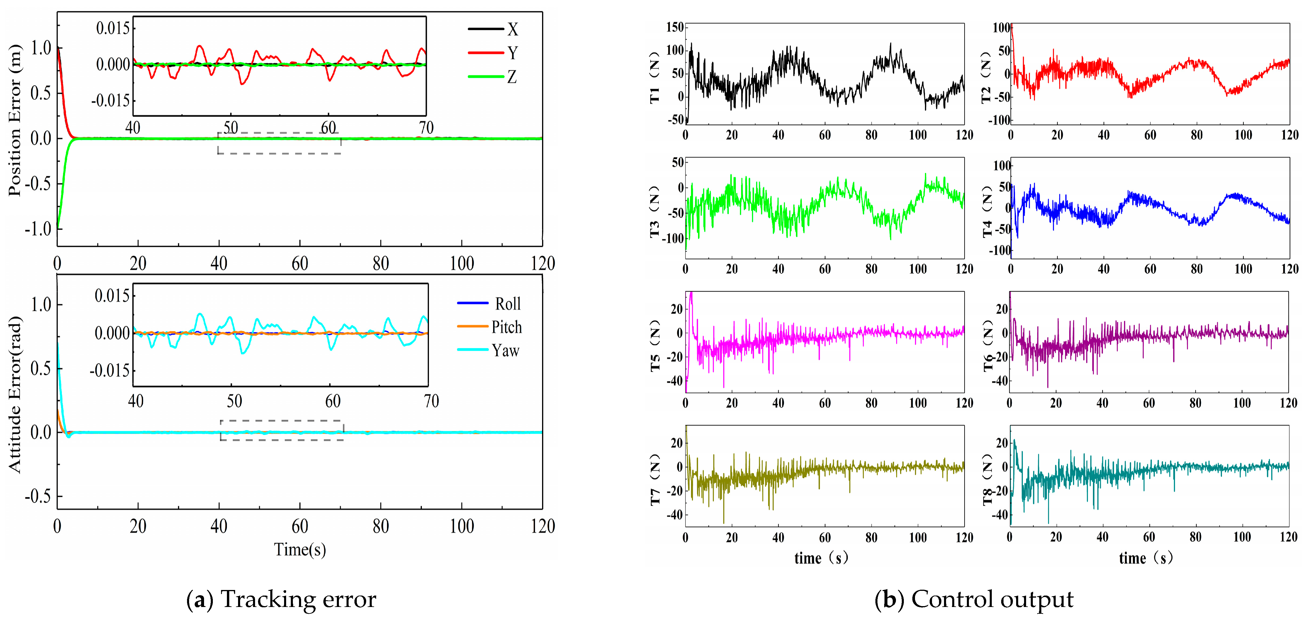
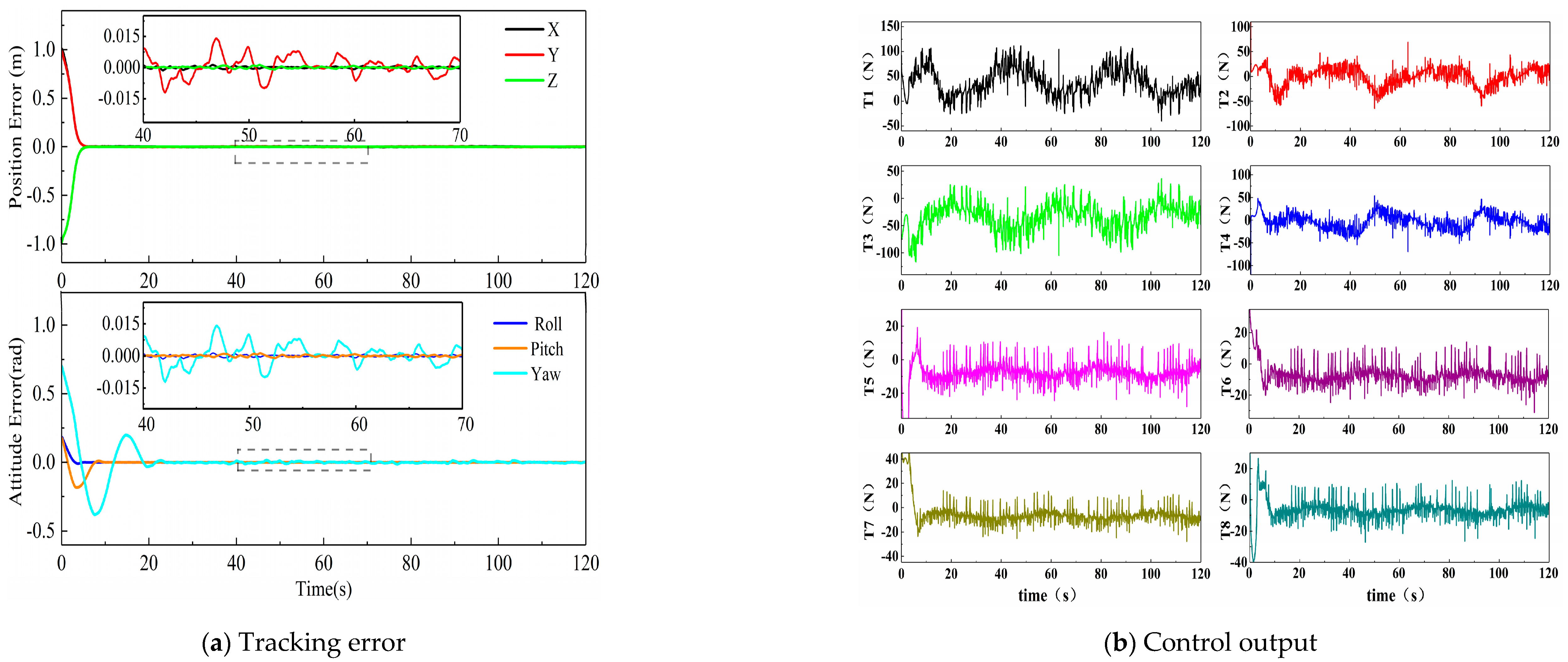
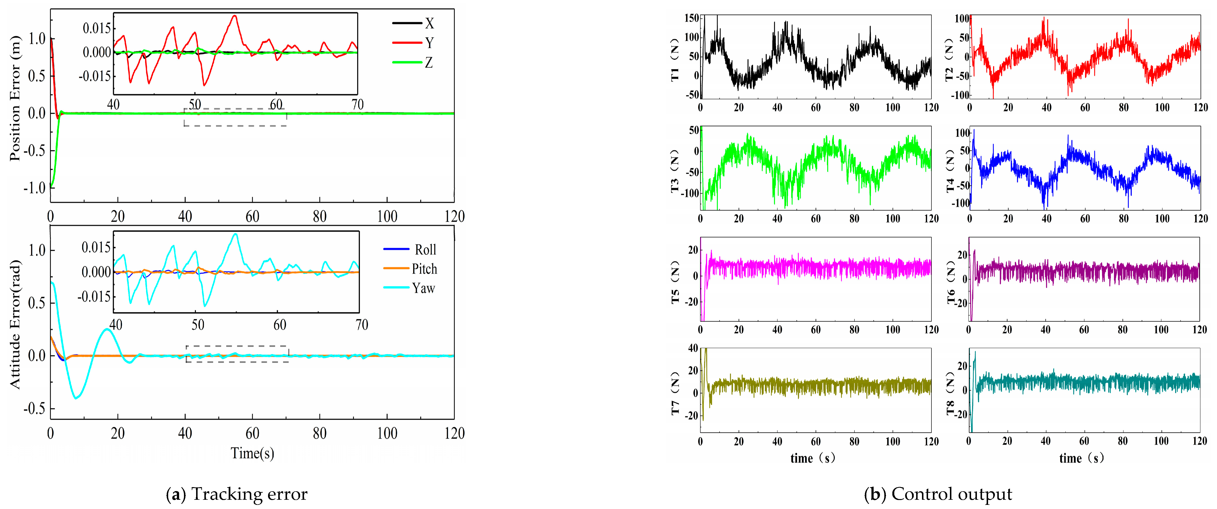
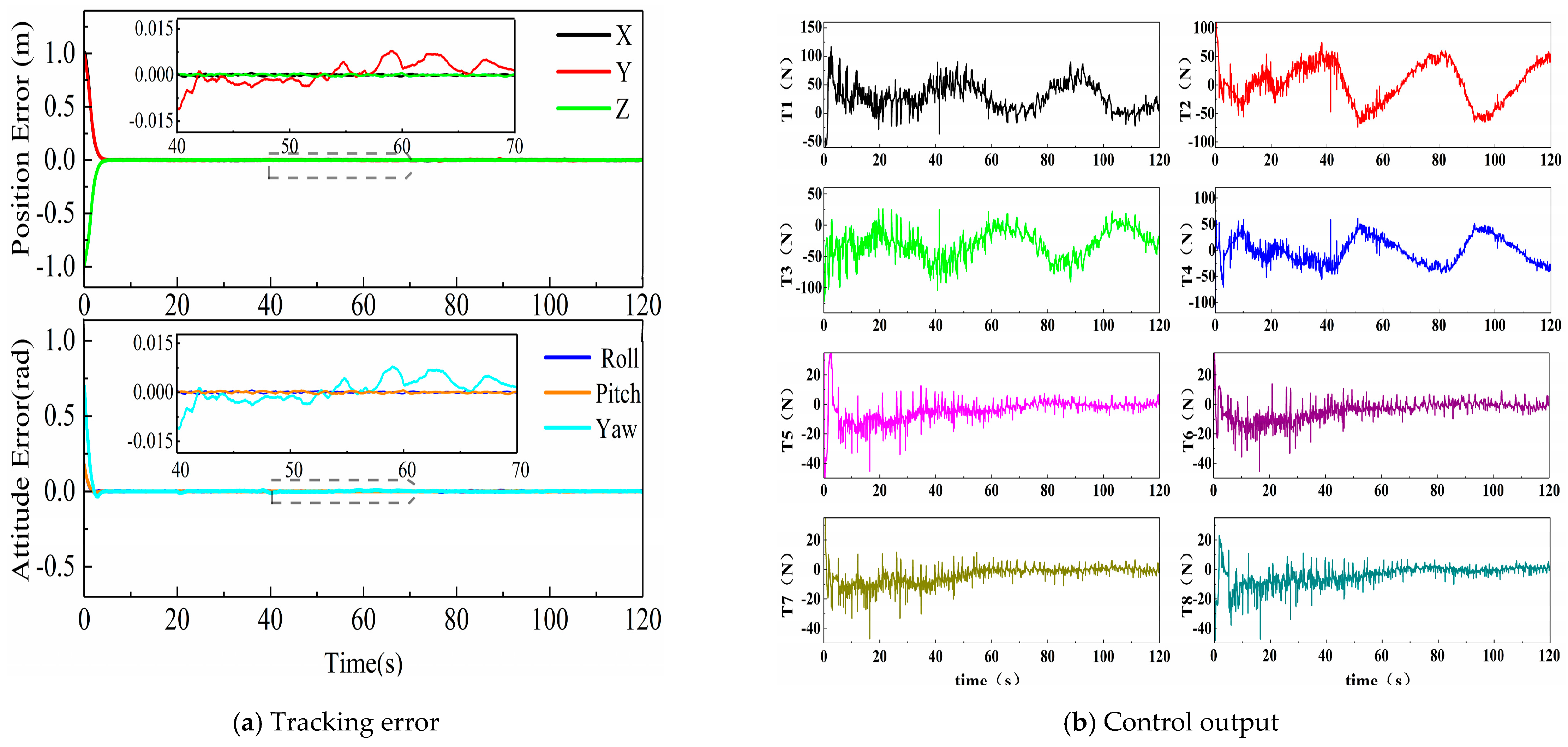
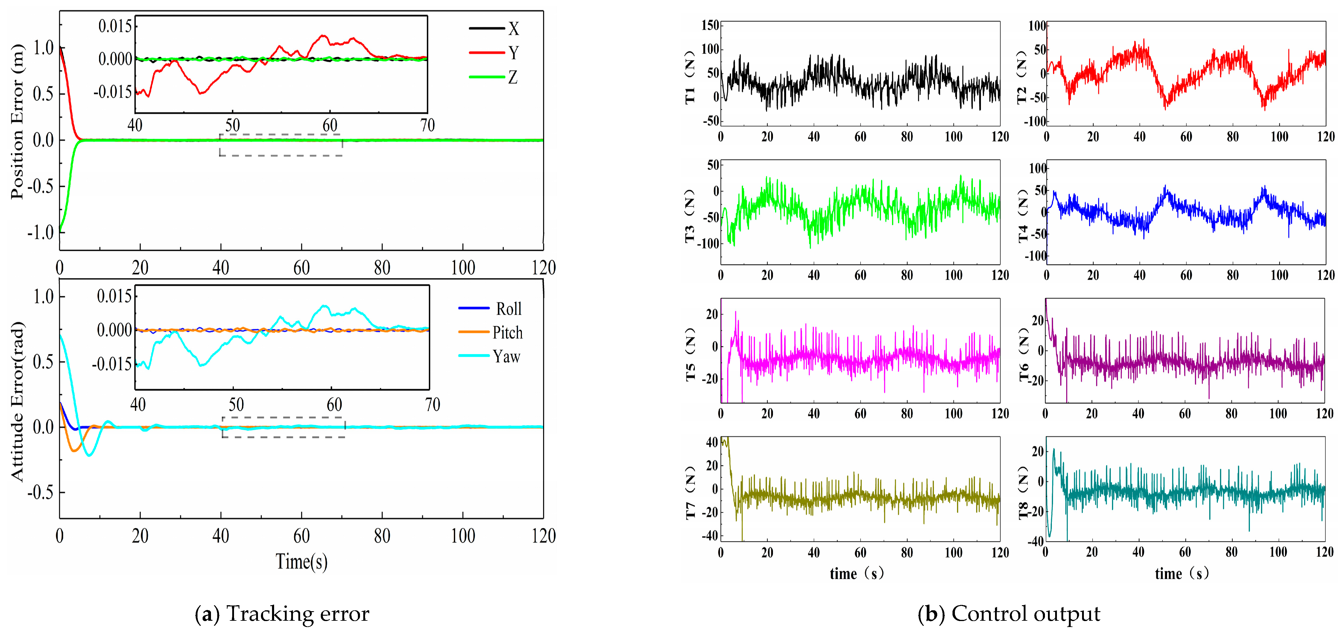
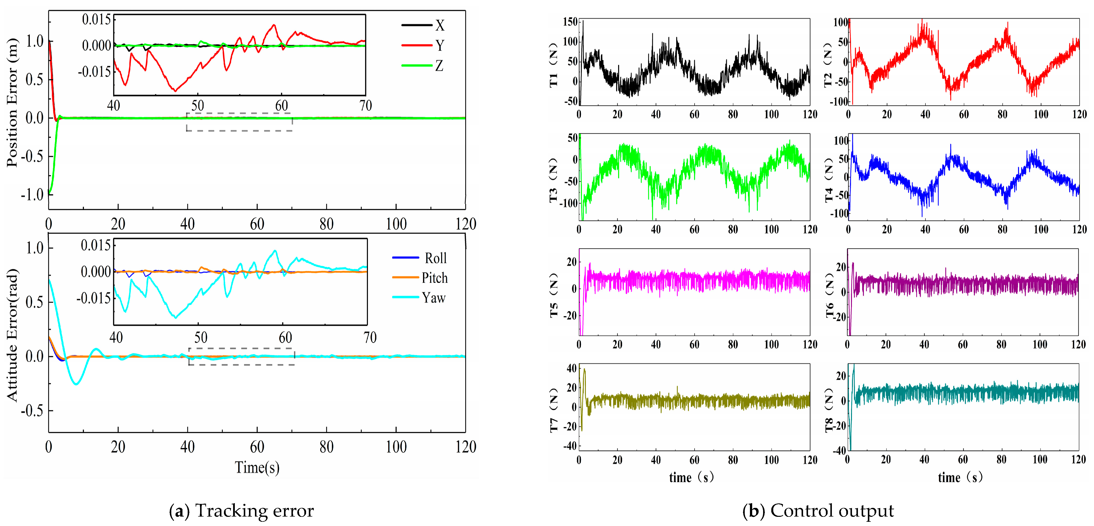
The simulation results of FTESO − FTC − APAM and FTESO − FTC and the compared method for Case 1 are presented in Figure 1, Figure 2 and Figure 3, respectively. In addition, the simulation results of these three methods for Case 2 are presented in Figure 4, Figure 5 and Figure 6, respectively. Finally, to fully illustrate the effectiveness of the method in this paper, the tracking results of these three methods for Case 3 are presented in

Table 1. Compared results of the three methods under Cases 1–3.

Methods	Tracking Error	Distance Errors (m)			SSCS (107 × N2)
		Case 1	Case 2	Case 3	Case 1	Case 2	Case 3
FTESO − FTC − PAM	Mean	0.0224	0.0227	0.0212	2.77	3.49	2.43
	Mean square error	0.1502	0.1522	0.1482
FTESO − FTC	Mean	0.0356	0.0367	0.0328	2.74	3.48	2.34
	Mean square error	0.1991	0.2008	0.1863
Compared method [23]	Mean	0.0225	0.0236	0.0215	3.81	4.71	3.07
	Mean square error	0.1516	0.1527	0.1496

.

Referring to [35], in this paper, the mean and mean square error of the absolute value of the tracking error were used to measure the tracking effect. If the chattering phenomenon in the control signals became serious, the energy consumption caused by the chattering of the control signal would be increased if the environmental parameters had no change, according to [36]. The energy consumption value was calculated by the sum of the squares of the control signal (SSCS), shown as follows:

$$SSCS={{\displaystyle \sum {\displaystyle \sum _{i=1}^8\left|u_i\right|}}}^2$$

(36)

For the convenience of analysis, this paper organizes and summarizes the mean, mean square error of the absolute value of the tracking error, and energy consumption (SSCS) in Case 1–Case 3 into Table 1.

In addition, in this paper, the position errors of the three degrees of freedom, X, Y, and Z, are synthesized into distance errors.

In terms of the tracking error and energy consumption, the simulation results of FTESO − FTC − APAM and FTESO − FTC and the compared method are analyzed.

Firstly, compared with the method in [23], the analysis of Cases 1–3 in Table 1 shows that FTESO − FTC has an obvious effect on reducing the energy consumption; however, the tracking accuracy was reduced. Taking Case 1 as an example, compared with the method in [23], the mean and mean square error of the distance error of FTESO − FTC increased by 58.22% and 31.33%, respectively, so the tracking accuracy decreased. However, it can be found that compared with the method in [23], FTESO + FTC reduced the energy consumption by 28.08%.

Compared with [23], it can be concluded that FTESO − FTC was effective at reducing the energy consumption, but there was the problem of reducing the tracking accuracy. Therefore, this paper proposed PAM based on FTESO − FTC to reduce the energy consumption of the control output while maintaining a good tracking accuracy.

Then, compared with FTESO − FTC, it can be seen from Cases 1–3 in Table 1 that FTESO − FTC − PAM significantly improved the tracking accuracy and slightly increased the energy consumption. Similarly, taking Case 1 as an example, compared with FTESO − FTC, FTESO − FTC − PAM reduced the mean value and mean square error of the distance error by 37.07% and 24.56%, respectively, that is, the tracking accuracy was significantly improved. FTESO − FTC − APAM was close to FTESO − FTC in terms of the energy consumption (slightly increased).

Furthermore, compared with the method in [23], it can be obtained from Cases 1–3 in Table 1 that FTESO − FTC − APAM can significantly reduce energy consumption on the premise of a slightly improved tracking accuracy. Then, taking Case 1 as an example, compared with [23], the mean value and mean square error of the absolute value of the distance error in the FTESO − FTC − APAM were slightly smaller, and the tracking accuracy was slightly improved. In terms of energy consumption, compared with the method in [23], FTESO − FTC − APAM was reduced by 29.92%, and the effect of reducing the energy consumption was obvious.

It can be concluded that FTESO − FTC − PAM was a further improved method based on the FTESO − FTC of this paper. Overall, based on the simulation results of the above three methods, it is concluded that compared with FTESO − FTC, the FTESO − FTC − PAM could greatly improve the tracking accuracy under the condition of a slight increase in energy consumption. Compared with the method in [23], the FTESO − FTC − PAM of this paper made up for the shortcomings of FTESO − FTC in reducing the tracking accuracy when reducing the energy consumption and finally could achieve the control goal of reducing the energy consumption while maintaining a better tracking accuracy.

6. Conclusions

This paper studies the problem of fault tolerant control for fully actuated AUV thrusters in the presence of current disturbances, thruster faults, and dynamic model uncertainty. In view of the problems of high energy consumption caused by the chattering of the control signal when the method in [23] is used in AUV, this paper proposes FTESO − FTC − PAM, i.e., a fault-tolerant control method based on a finite-time extended state observer for AUV with unknown thruster faults. Through theoretical analysis and simulation experiments, the following conclusions can be drawn.

(1) Aiming at the problem of large energy consumption when a previous method is applied to AUVs, this paper proposes the FTC method based on FTESO (FTESO − FTC). In this paper, the design of the FTESO and the FTC adopts ISMS and NFTSMS, respectively. The stability of the finite-time extended state observer and the finite-time convergence of the closed-loop control system formed by the fault-tolerant control method are proved by the Lyapunov stability theory. The simulation comparison experiment results using an ODIN AUV show that under the simulated thruster fault and ocean current interference, FTESO − FTC is more effective at reducing the energy consumption than the method in [23], but it has the problem of reducing the accuracy of tracking.

(2) To this end, the above-mentioned FTESO − FTC is further improved, and the parameter adjustment method (PAM) for AUV thrusters is added. The simulation and compared experimental results for the ODIN AUV show that after adding PAM, the tracking accuracy can be effectively restored, and the energy consumption is basically not increased. Moreover, the simulation results show that the FTESO − FTC − PAM is superior to the method in [23] in terms of reducing the energy consumption and improving the tracking accuracy.