Typhoon Wave Simulation Responses to Various Reanalysis Wind Fields and Computational Domain Sizes

Abstract

A fully coupled tide-surge-wave model was developed to study the influence of different computational domains on typhoon wave characteristics in the waters surrounding Taiwan. Three typhoons were selected as study cases: Meranti, Malakas, and Megi, which successively impacted Taiwan in September 2016. Superposition of the CFSV2 winds blended with ERA5 winds onto the tide-surge-wave model yielded optimum simulations of typhoon waves. Storm wave responses along the eastern shelf of Taiwan resulting from three typhoons were examined in four model domains. The first domain (D01) was primarily situated in the region where giant waves were generated. The second domain (D02) covered an area extending from 114° E to 130° E and 19° N to 29° N. The third domain (D03) southwardly included the entire Bashi Channel, from longitudes of 111° E to 135° E and latitudes of 18° N to 30° N. The fourth domain (D04) was the largest among the four computational domains; it extended from longitudes of 105° E to 140° E and latitudes of 15° N to 31° N. The simulated sea state responses indicated that the smaller computational domains were inadequate for typhoon-driven storm wave computation purposes, although the areas of D01 and D02 reached approximately 0.75 and 1.38 million km², respectively, encompassing all of Taiwan Island and adjacent waters. Our results suggest that utilizing at least D03 or a larger model domain (e.g., D04) is essential to account for the remote wind effect of typhoons on wave simulations in Taiwanese waters.

1. Introduction

In the Northwestern Pacific Ocean, one of the most active typhoon areas worldwide, extreme typhoon-driven waves and storm surges are responsible for significant geomorphic changes, severe flooding, and property damage in coastal regions [1,2,3,4]. Taiwan is an island country in East Asia, located at the junction between the East and South China Seas in the Northwestern Pacific Ocean; thus, it is necessary to develop a fully coupled tide-surge-wave prediction system covering the waters surrounding Taiwan and adjacent small islands, to implement early measures against typhoon-induced coastal disasters. This is particularly true for the prediction or simulation of typhoon-driven waves, because extreme typhoon waves are more severe than storm surges and can threaten human lives and the infrastructure of Taiwan’s coastal communities; for example, substantial storm waves destroyed a lighthouse in a fishing port on the southeastern coast of Taiwan during Typhoon Meranti in 2016 [5].

Currently, numerical models have become helpful tools and have been widely used to assess the physics of either continental margins or offshore waters. However, it is crucial to recognize that the various elements comprising a numerical model might affect the simulated responses of extensive waters, including the model governing equations, model boundary conditions (e.g., meteorological and hydrological conditions), model forcing functions, model numeric scheme, model grid structure or type, and model computational domain size [6]. The influence of boundary conditions on the simulated results can be jointly considered with computational domain size determination. A significant disadvantage in typhoon wave and surge modeling studies is the lack of adequate research to indicate convergence concerning the grid structure, grid spacing, and computational domain size. Consequently, it is often unclear whether computed water body responses are significantly aliased, due to an inadequate grid resolution, or are overwhelmed by the imposed boundary conditions and their interactions with the selected domain. To eliminate the effects of the selected boundary conditions on model simulations, the computational domain for storm surge, storm tide and storm wave modeling must be large enough to accommodate an entire typhoon, including its peripheral circulation [7,8,9,10,11,12,13].

Many previous studies have demonstrated that the computational domain size could influence storm surge simulations [6,14,15]. Blain et al. [6] indicated that if the offshore boundary was located in an area with significant surges, the nearshore surge elevation would be underestimated because a storm surge at the boundary is difficult to estimate in advance. Similar to the storm surge simulation results obtained by Blain et al. [6], typhoon wave simulation accuracy could theoretically increase with an increasing computational domain size, and primary storm waves are only accurately simulated when the offshore boundary is located far from the study area. Additionally, the computational domain should be large enough to capture the resonant modes. However, a critical issue that remains unresolved is the appropriate size of the model domain at a given geographic location, and specific typhoon conditions. Moreover, previous studies only focused on the influence of the domain size on storm surge simulations, but there is a lack of relevant studies on the effect of the domain size on storm wave simulations.

The present study aimed to systematically and quantitatively investigate the influence of the computational domain size on simulated typhoon waves. Three actual typhoons, which traversed the southern and eastern waters of Taiwan and made landfall on the eastern coast of Taiwan, were applied in storm wave simulations using three reanalysis wind fields in the present study, considering four model domains. Each computational domain exhibited a different size and covered an increasingly larger region. Details of the materials and methods are described in the following section; the typhoon wave simulation results obtained with the different model domain sizes and reanalysis winds are presented in Section 3. In Section 4, a further discussion of the present study is given, and a summary and conclusions are outlined in Section 5.

2. Materials and Methods

2.1. Three Successive Typhoon Events

Typhoon Meranti, referred to as Typhoon Ferdie in the Philippines, was one of the most intense tropical cyclones on record. Impacting the Batanes in the Philippines, Taiwan, and Fujian Province of China in September 2016, Meranti became a tropical depression on 8 September near the island of Guam. Tracking towards the west–northwest, Meranti gradually intensified until 11 September, at which point it entered a period of rapid intensification. Continuing to rapidly intensify, it became a super typhoon early on 12 September, as it passed through the Luzon Strait, ultimately reaching its peak intensity on 13 September with 1-min sustained winds of 315 km/h. Shortly afterward, it passed directly over the island of Itbayat. Meranti passed to the south of Taiwan as a super typhoon and steadily weakened due to land interaction. By 15 September, it reached Fujian Province as a Category 2-equivalent typhoon, becoming the strongest typhoon on record to impact the province. Upon moving inland, a rapid weakening ensued, and Meranti degraded to reach the extratropical level the day after it passed to the south of the Korean Peninsula. The tracks and arrival time (UTC+0) of Typhoon Meranti are shown in Figure 1a.

Typhoon Malakas acquired a very favorable sea surface temperature (SST) of nearly 30 °C and was later upgraded to a Category 2 typhoon by 15 September. After maintaining this intensity for six hours, satellite imagery depicted enhanced deep convection and a well-defined 18.5-km eye feature as Malakas rapidly intensified into a Category 4 typhoon. Malakas reached its peak intensity with 1-min sustained winds of 215 km/h and a minimum pressure of 930 hPa. The Japan Meteorological Agency (JMA) recorded 10-min sustained winds of 175 km/h at midnight on 17 September. Shortly thereafter, its eye became cloud-filled and uneven, and it weakened into a Category 3 typhoon. Later that same day, Malakas further weakened to reach the Category 2 level, as satellite imagery depicted warming cloud tops, decreasing convection, and an SST of approximately 28 °C. However, by 18 September, Malakas again started to intensify as it moved east–northeastward. Malakas reached its secondary peak on 19 September but only as a Category 3 typhoon. Malakas then started to weaken due to land interaction with Japan. On 20 September, the Joint Typhoon Warning Center (JTWC) downgraded Malakas to a tropical storm, while the JMA downgraded it to a severe tropical storm because at approximately 00:00 JST on 20 September (15:00 UTC on 19 September), Malakas made landfall over the Ōsumi Peninsula in Japan. It subsequently crossed Cape Muroto at approximately 11:00 JST (02:00 UTC) and made landfall over Tanabe at approximately 13:30 JST (04:30 UTC). The JAM and JWTC issued their final advisory as it became an extratropical system later that day. The tracks and arrival time (UTC+0) of Typhoon Malakas are shown in Figure 1b.

Typhoon Megi, referred to as Typhoon Helen in the Philippines, was a large and powerful tropical cyclone affecting Taiwan and eastern China in late September 2016. The JMA upgraded a tropical depression to a tropical storm and named it Megi early on 23 September, when the JTWC indicated that monsoonal circulation had consolidated, upgrading it to a tropical depression, but lacking a definitive center. Six hours later, the JTWC upgraded Megi to a tropical storm. When formative banding and cloud tops were improving and cooling late on the same day, the JMA further upgraded the broad system to a severe tropical storm. Megi was trying to form an eye, prompting both the JMA and JTWC to upgrade the system to a typhoon on 24 September. After completing an eyewall replacement cycle on 26 September, Megi eventually strengthened in the afternoon, resulting in an uneven but much larger eye embedded in this large typhoon. The JMA indicated that Megi had reached its peak intensity at 18:00 UTC, with ten-minute maximum sustained winds of 155 km/h and a central pressure of 940 hPa. Megi’s large eye temporarily became more defined early on 27 September; however, the eye soon became cloud-filled as the typhoon approached the eastern coast of Taiwan. Shortly before Megi made landfall over Hualien city at 14:00 Taiwan Time (06:00 UTC), it had already intensified into a stronger typhoon at approximately 03:00 UTC, with one-minute maximum sustained winds of 220 km/h indicated by the JTWC, equivalent to Category 4 on the Saffir–Simpson hurricane wind scale. Subsequently, interaction with the high mountains in Taiwan caused Megi to significantly weaken, and the typhoon entered the Taiwan Strait from Yunlin County, Taiwan, at 21:10 Taiwan Time (13:10 UTC). At 04:40 CST on 28 September (20:40 UTC on 27 September), Megi made landfall over Huian County of Fujian Province, China, as a minimal typhoon. The tracks and arrival time (UTC+0) of Typhoon Megi are shown in Figure 1c.

2.2. Measurements of the Significant Wave Height via Wave Buoys

Data recorded by four wave buoys deployed in the offshore eastern waters of Taiwan were selected to validate the model performance in regard to storm wave simulation with different computational domains. According to the location of the buoys, from north to south, they included the Suao, Hualien, Taitung, and Eluanbi buoys (as shown in Figure 1b). Annual buoy observation data of the Central Weather Bureau, Taiwan, indicate that the sampling frequency of these wave buoys reaches 2 Hz over 10 min at the beginning of each hour, and the accuracy of significant wave height measurement is ±10 cm.

Table 1. Scenario simulations conducted in the present study.

Buoy Name	Lon. (°E)	Lat. (°N)	Water Depth (m)
Suao	121.8758	24.6247	23
Haulien	121.6325	24.0311	22
Taitung	121.1400	22.7222	30
Eluanbi	120.8225	21.9003	40

Data source: Central Weather Bureau and Water Resource Agency of Taiwan.

lists the coordinates of the four wave buoys and their corresponding water depths.

2.3. Sources of the Meteorological Conditions for the Sea State Simulations

The Cross-Calibrated Multi-Platform (CCMP) is a near-global dataset for gridded surface vector winds. The CCMP is produced using a combination of ERA-40 reanalysis and European Center for Medium-Range Weather Forecasting operational analysis data as background wind data, and wind data acquired by satellites and moored buoys [16]. CCMP products provide a consistent, gap-free long-term time series of wind vector analysis fields over the ocean surface from 1987 to the present, with a spatial resolution of 0.25° and a temporal resolution of 6 h. A near-real-time (NRT) version of the CCMP (hereafter referred to as CCMPNRT) was developed to overcome the obstacles raised by a delay in reanalysis fields available only after several months and measurements delay of in situ sources. Two changes were made to the input datasets of the CCMPNRT: the background winds now comprised operational 0.25° analysis winds retrieved from the National Centers for Environmental Prediction (NCEP) global data assimilation system, and no in situ data were used. These modifications allowed the CCMPNRT to be routinely processed with a latency of less than 48 h [17]. The CCMPNRT is available at 0.25° spatial and 6 h temporal resolutions, with a delay of only a few hours.

The NCEP Climate Forecast System (CFS) was upgraded to version 2 (hereafter referred to as CFSV2) and became operational at the NCEP in March 2011. CFSV2 is the same model used to create the NCEP Climate Forecast System Reanalysis (CFSR) product. CFSV2 is with no doubt superior to the CFS, especially at the intraseasonal time scale; it also provides many more subseasonal and seasonal forecasting products with an extensive set of retrospective forecasts for users to calibrate their forecast products [18]. CFSV2 products are available at spatial resolutions of 0.2°, 0.5°, 1.0°, and 2.5° and hourly intervals. In the present study, hourly winds with a spatial resolution of 0.2° were utilized in typhoon wave simulations.

ERA5 is the fifth-generation European Centre for Medium-Range Weather Forecasts (ECMWF) atmospheric reanalysis dataset of the global climate. It combines vast amounts of historical observations into global estimates using advanced modeling and data assimilation systems. ERA5 provides hourly estimates of a large number of atmospheric, land, and oceanic climate variables, and includes information on the uncertainty in all variables. These reanalysis data cover the Earth via a 0.25° (approximately 30-km) grid and resolve the atmosphere using 137 levels from the surface up to 80 km. ERA5 publishes quality-assured monthly updates within three months of real time. Compared to ERA-Interim, the hourly output resolution of ERA5 represents a notable improvement, and provides a more detailed evolution of particular and severe weather events, e.g., typhoons.

The dynamic wind fields of the above three successive typhoons extracted from the CCMPNRT, CFSV2, and ERA5 were applied in storm wave simulations in the present study. These gridded winds were converted into unstructured grids of the SCHISM-WWM-III via the inverse distance weighting (IDW) method.

2.4. Configuration of the SCHISM-WWM-III with Four Computational Domains

The Semi-implicit Cross-scale Hydroscience Integrated System Model (hereafter referred to as SCHISM) developed by Zhang et al. [19] was chosen to function as a hydrodynamic model in the present study. Similar to its predecessor, the Semi-implicit Eulerian–Lagrangian Finite Element/volume (SELFE) model (developed by Zhang and Baptista [20]), the SCHISM is also based on unstructured meshes with a no-mode-splitting technique to eliminate the numerical errors resulting from splitting between internal and external modes [21]. The SCHISM applies a highly efficient semi-implicit scheme to the treat advection terms of momentum equations, and consequently bypasses the Courant–Friedrichs–Lewy (CFL) condition, the severest stability constraint of numerical modeling [22]. The two-dimensional module of the SCHISM (SCHISM-2D) was utilized in the present study because a two-dimensional model is sufficient to reproduce typhoon-driven hydrodynamics in the nearshore and offshore waters of Taiwan [7,8,9,10,11,23,24,25,26]. The SCHISM and SELFE modeling systems are highly scalable and extendable and seamlessly connect large and small domains; these superiorities make these models multipurpose modeling systems. For example, inundation assessments of coastal regions [27,28], hydrodynamic and water quality simulations of estuarine systems [29,30,31], and tidal current power evaluations [32,33] have been conducted.

We preset a Manning’s coefficient value of 0.025 with a time step of 120 s in SCHISM-2D based on the bathymetric characteristics of the waters surrounding Taiwan and the numerical stability of SCHISM-2D.

A third-generation spectral wind wave model, the Wind Wave Model version III (WWM-III), functioned as a sea state simulator in the present study. The WWM-III is an upgraded version of the WWM-II (developed by Roland et al. [34]), which employs a fractional step method to solve the wave action balance equation on unstructured grids. The wave breaking phenomenon attributed to the depth in nearshore shallow waters was treated with the BJ 78 model (proposed by Battjes and Janssen [35]). The Joint North Sea Wave Project (JONSWAP, Hasselmann et al. [36]) applied a peak enhancement coefficient value of 3.3 in wave spectra, which is also adopted in the WWM-III, and the wave breaking criterion was set to 0.78, while the bottom friction coefficient was set to 0.067. The number of bins in the directional space reaches 36 to consider a full circle of 360°, which suggests that the spectral directional resolution of the WWM-III is 360°/36 = 10°. Additionally, 36 frequency bins were utilized to divide the discrete wave period from 0.03 to 1.0 Hz.

An identical domain decomposition scheme is employed in both SCHISM-2D and WWM-III; hence, this prevents the interpolation errors of these two models by sharing the same subdomains. By adopting time steps of 120 s for SCHISM-2D and 600 s for the WWM-III, the parallelization, two-way, tightly coupled modeling system of the SCHISM-WWM-III is very computationally efficient. The SCHISM-WWM-III has been widely used to simulate typhoon-generated coastal storm tides and offshore storm waves in Taiwanese waters [5,7,8,9,10,11,25,37].

The GEBCO_2022 Grid product is the latest gridded global bathymetric product released by the General Bathymetric Chart of the Oceans (GEBCO). GEBCO_2022 provides a global coverage of elevation data in ocean and land regions (in meters) at a spatial resolution of 15 arc-seconds. Gridded bathymetric and topographic data were extracted from the global GEBCO_2022 Grid product and interpolated into the unstructured grids of the SCHISM-WWM-III.

Four computational domains of significantly varying sizes were considered in the present investigation. Different domain sizes were applied to demonstrate the influence of the computational domain size on typhoon wave simulations. The two smaller domains (domains 01 and 02, i.e., D01 and D02, respectively,) were constructed to facilitate comparison to the two larger domains (domains 03 and 04, i.e., D03 and D04, respectively,) used in recent storm wave modeling efforts. All domains created in the present study expand outward from the traversed water region of the three successive typhoons around Taiwan and increasingly cover more extensive areas (as shown in Figure 2).

Table 2. Characteristics of computational domains D01 to D04.

Domain Number	Coverage (km2)	Nodes	Elements
D01	0.75 × 106	77,505	149,658
D02	1.38 × 106	101,945	198,270
D03	2.50 × 106	168,829	327,955
D04	4.48 × 106	276,639	540,510

summarizes the coverage levels and characteristics of the four computational domains. As these four computational domains entirely encompass the path of the above three successive typhoons when they passed or made landfall over Taiwan, open wave boundary conditions were not essential for the SCHISM-WWM-III [7,8,9,11].

The TPXO is a barotropic tide model obtained using the methods proposed by Egbert et al. [38] and Egbert and Erofeeva [39]. These methods have been implemented in the OSU Tidal Inversion Software (OTIS) package. All of the global/regional/local TPXO models can be used with OTIS by assimilating satellite altimetry and sometimes other data. Three variables, including the elevation, velocity, and transport, are included in both global and regional tidal models. TPXO9-atlas is the latest fully global tide model with a spatial resolution of 1/30 degrees for all coastal areas, including the Arctic and Antarctic. Therefore, the horizontal velocity and tidal elevation along the SCHISM-WWM-III open boundaries were driven by eight main tidal constituents (M2, S2, N2, K2, K1, O1, P1, and Q1) extracted from the TPXO9-atlas tidal model. Anomalous sea surface elevations generated by atmospheric pressure are also considered in the SCHISM-WWM-III.

3. Results

3.1. Influence of the Different Wind Fields on the Simulation of the Typhoon-Driven Significant Wave Height

Figure 3, Figure 4 and Figure 5 show scatter plots to compare significant wave height between the measurement and simulation data and the hourly difference for the Suao, Hualien, Taitung, and Eluanbi wave buoys using CCMPNRT (Figure 3), CFSV2 (Figure 4), and ERA5 (Figure 5) wind fields. The hourly differences in significant wave height between the measurement and simulation data for the four wave buoys employing the D04 computational domain of the SCHISM-WWM-III with CCMPNRT winds are shown in Figure 3. The hourly difference in the maximum wave height reached approximately 4.0 m for the Suao (Figure 3a) and Eluanbi (Figure 3d) wave buoys during Typhoon Megi; however, the differences reached approximately 2.5 and 2.0 m for the Hualien (Figure 3b) and Taitung wave buoys (Figure 3c), respectively. The Typhoon Megi-induced extreme wave height could reach 12.0 and 10.5 m at the Suao and Hualien wave buoys, respectively, while the CCMPNRT winds only resulted in a wave height smaller than 8.0 m at the Suao and Hualien wave buoys (Figure 3a and Figure 3b, respectively). Comparison of the Taitung and Eluanbi wave buoys (Figure 3c and Figure 3d, respectively) also revealed a phenomenon similar to that observed for the Suao and Hualien wave buoys. The SCHISM-WWM-III with CCMPNRT winds underpredicted Typhoon Meranti causing maximum wave heights of 2.5 and 4.0 m at the Taitung and Eluanbi wave buoys, respectively. Overall, the wave heights predicted considering CCMPNRT winds were inferior; the maximum hourly differences could reach 8.0 and 7.0 m higher at the Taitung and Eluanbi wave buoys, respectively.

The performance of the SCHISM-WWM-III paired with CFSV2 winds in significant wave height simulations during Typhoons Meranti, Malakas, and Megi were evaluated based on measurements recorded at the Suao, Hualien, Taitung, and Eluanbi wave buoys. The hourly differences between the simulation and observation data are shown in Figure 4. The maximum typhoon wave height simulations were better than those using CCMPNRT winds. The SCHISM-WWM-III with CFSV2 winds underpredicted the Typhoon Megi and Meranti-driven extreme waves by approximately 4.0 m (Figure 4a), 1.5 m (Figure 4b), and 1.0 m (Figure 4d) at the Suao, Hualien, and Eluanbi wave buoys, respectively. However, a wave height overprediction of 2.0 m could be observed for Typhoon Meranti, triggering an enormous wave at the Taitung wave buoy (Figure 4c). The maximum hourly differences in significant wave height between the simulation and measurement data reached approximately 4.0, 5.0, 11.0, and 12.0 at the Suao, Hualien, Taitung, and Eluanbi wave buoys, respectively. Significant differences were obvious for wave heights larger than 6.0 m (as shown in Figure 4a–d).

Imposing ERA5 winds on the SCHISM-WWM-III yielded negligible hourly differences in the simulated significant wave height among the three dynamic wind fields, except for very high waves above 10.0 m (as shown in Figure 5a–d). The maximum hourly differences in significant wave height between the simulation and measurement data reached approximately 4.0 and 3.5 m at the Suao (Figure 5a) and Hualien (Figure 5b) wave buoys, respectively, during the Typhoon Megi period. The maximum differences were more pronounced and reached up to 7.0 and 11.0 m at the Taitung (Figure 5c) and Eluanbi (Figure 5d) wave buoys, respectively, during the passage of Typhoon Meranti. Overall, ERA5 winds produced significant wave heights which were more closely matching the measurements than those produced by CCMPNRT and CFSV2 winds, especially for wave heights smaller than 6.0 m; however, underestimations could occur if typhoons generated more intense winds.

To visualize which of several approximate representations or models of a given system, process, or phenomenon is most realistic, Taylor [40] designed a mathematical diagram, namely, the Taylor diagram. Taylor diagrams thus facilitate a comparative assessment of different models by quantifying the degree of correspondence between the modeled and observed behaviors in terms of three statistics: the correlation coefficient, root-mean-square error, and standard deviation. Although Taylor diagrams have primarily been used to evaluate models developed to study climate processes and other aspects of the Earth’s environment [41], they can also be adopted for purposes unrelated to Earth systems or environmental science. Figure 6a–d show Taylor diagrams of the relative bias, correlation coefficient, and normalized standard deviation patterns between the in situ observations and model simulations of the significant wave height using the ERA5 (No. 1 in Figure 6a–d), CFSV2 (No. 2 in Figure 6a–d), and CCMPNRT (No. 3 in Figure 6a–d) wind fields for the Suao (Figure 6a), Hualien (Figure 6b), Taitung (Figure 6c), and Eluanbi (Figure 6d) wave buoys. The correlation coefficient and normalized standard deviation of the three wind fields are shown in Figure 6a–d. The normalized standard deviation indicates the relative amplitude of the modeled and observed variations. Moreover, the correlation coefficient measures the linear dependence correlation between two variables. The quantitative analysis results derived using the Taylor diagram method indicated that the significant wave height simulations utilizing the combination of ERA5 winds and the SCHISM-WWM-III yielded the minimum statistical errors, and the corresponding results occurred closest to the reference line (No. 1 in Figure 6a–d), followed by the employment of CFSV2 and CCMPNRT winds.

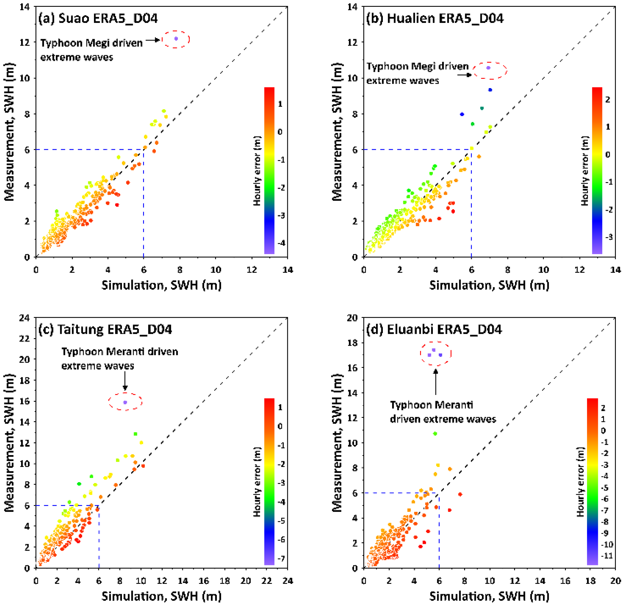
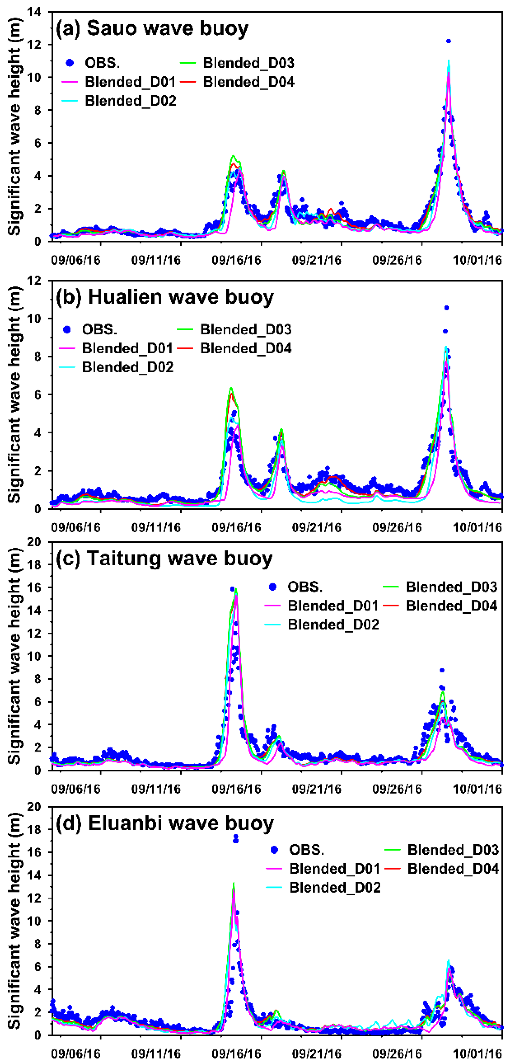
3.2. Influence of the Different Computational Domains on the Simulation of the Typhoon-Driven Significant Wave Height

Through qualitative and quantitative analysis of the significant wave height simulations conducted in the largest computational domain (i.e., D04), the SCHISM-WWM-III driven by ERA5 wind fields exhibited an overall high reliability in simulating the storm wave height, although vast storm waves were still underestimated. Thus, considering the four computational domains, ERA5 winds were superimposed on the SCHISM-WWM-III to examine the sensitivity of typhoon wave simulations to the model domain size. The Taylor diagram method was again applied to enable a comparative evaluation of the four computational domains in significant wave height simulations during the above three successive typhoon events; the modeling coverage in ascending order is D01, D02, D03, and D04. Figure 7 shows Taylor diagrams for the comparison of the simulated typhoon-induced significant wave heights at the Suao (Figure 7a), Hualien (Figure 7b), Taitung (Figure 7c), and Eluanbi (Figure 7d) wave buoys. Domains 01, 02, 03, and 04 are indicated as No. 1, No. 2, No. 3, and No. 4, respectively, in Figure 7a–d. As shown in Figure 7a–d, domain 04 (No. 4) exhibited the minimum statistical errors in the significant wave height simulations, and the corresponding results occurred closest to the reference line, followed by the utilization of domains 03, 02, and 01. However, the adoption of domains 03 and 04 generated negligible statistical errors in the typhoon wave simulations.

A two-dimensional spatial distribution map was used to compare the simulated significant wave height among the different computational domains. Figure 8, Figure 9, Figure 10 and Figure 11 show the ocean surface storm waves generated by Typhoon Meranti at 00:00 on 14 September (Figure 8a, Figure 9a, Figure 10a and Figure 11a), Typhoon Malakas at 00:00 on 17 September (Figure 8b, Figure 9b, Figure 10b, and Figure 11b), and Typhoon Megi at 00:00 on 27 September (Figure 8c, Figure 9c, Figure 10c and Figure 11c) using computational domain 01 (D01, Figure 8), computational domain 02 (D02, Figure 9), computational domain 03 (D03, Figure 10), and computational domain 04 (D04, Figure 11), while ERA5 wind fields functioned as meteorological conditions for these four model domains. The plan views of the storm waves revealed an asymmetric distribution, and the coverage of very high waves was mainly concentrated on the right-hand side of the typhoon path because the total wind speed is the sum of the forward speed and local wind speed; in contrast, the total wind speed on the left-hand side of the typhoon path is the wind speed minus the forward speed. As shown in Figure 8, Figure 9, Figure 10 and Figure 11, the four domains produced similar patterns of the spatial distribution of typhoon waves larger than 9.0 m. However, the extent of large waves was restricted within computational domain 01 (D01, Figure 8c) because a small model domain cannot sufficiently contain typhoons of a large size. This phenomenon was evident in the storm wave simulations of the large-size Typhoon Megi (comparing Figure 8c to Figure 9c, Figure 10c and Figure 11c). Additionally, the effect of the boundary conditions on the spatial distribution of storm wave simulations was observed in the smallest model domain, i.e., domain 01 (D01, Figure 8a–c).

Another notable phenomenon was that wave heights between 7.0 and 8.0 m occurred in the southwestern offshore waters of Taiwan using computational domain 03 (D03) and computational domain 04 (D04) when Typhoon Megi was approaching Taiwan Island (as shown in Figure 10c and Figure 11c, respectively). However, the employment of smaller computational domains, i.e., D01 and D02, could not produce an analogous phenomenon to that observed for the larger computational domains, i.e., D03 and D04 (comparing Figure 8c to Figure 9c, Figure 10c and Figure 11c).

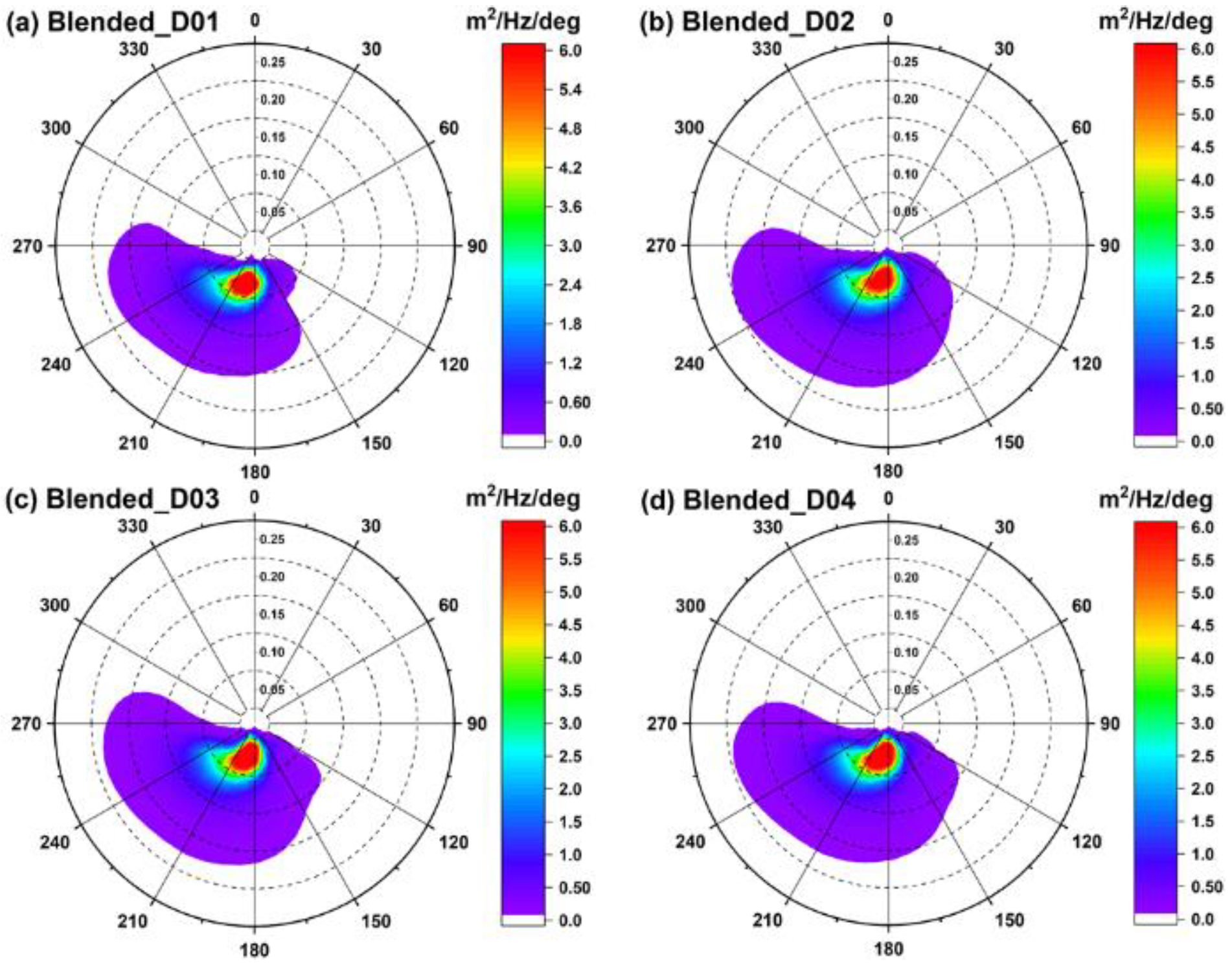
3.3. Influence of the Different Computational Domains on the Simulation of the Typhoon-Driven Wave Period and Wave Direction

Although the SCHISM-WWM-III forced by ERA5 winds produced the overall minimal statistical error in typhoon wave simulations over those driven by CCMPNRT and CFSV2 winds, the underprediction of typhoon-induced extremely large waves remained significant (as shown in Figure 5a–d). The direct modification approach proposed by Pan et al. [42] was therefore applied in the present study to take advantage of the combination of the CFSV2 (with the minimum errors in extremely large wave simulations) and ERA5 (with the minimum errors in overall wave simulations) wind fields to construct a suitable scale for the entire typhoon wind field:

$$W_{BL}=\{\begin{array}{cc}{W}_{ERA5}\left[\frac{r}{R_{Emax}}\left(\frac{W_{Cmax}}{W_{Emax}}-1\right)+1\right]\hfill & \hfill r<R_{Emax}\\ W_{ERA5}\left[\frac{R_{trs}-r}{R_{trs}-R_{Emax}}\left(\frac{W_{Cmax}}{W_{Emax}}-1\right)+1\right]\hfill & \hfill R_{Emax}\le r\le R_{trs}\\ W_{ERA5}\hfill & \hfill r>R_{trs}\end{array},$$

(1)

where W_BL is the wind speed at an arbitrary grid point within the model domain through the direct modification method, W_ERA5 is the wind speed extracted from ERA5 at an arbitrary point in the computational grid, W_Cmax and W_Emax are the maximum wind speed of the typhoon among the hourly ERA5 and CFSV2 wind fields, respectively, r is the radial distance from an arbitrary grid point within the model domain to the eye of the typhoon, R_trs is the radius of the modified scale (also referred to as the radius of the transitional zone), and REmax is the distance to the point of the maximum typhoon wind speed in the ERA5 wind field. Time-series significant wave height comparisons between the model simulation and measurement data for the Suao, Hualien, Taitung, and Eluanbi wave buoys using the four computational domains are shown in Figure 12a–d. Computational domain 03 produced typhoon significant wave heights very close to those calculated with computational domain 04. However, the blended typhoon wind fields still failed to capture the enormous waves generated by Typhoon Meranti at the Eluabi wave buoy (Figure 12d) and those induced by Typhoon Megi at the Suao, Hualien, and Taitung wave buoys (Figure 12a–c). Overall, the utilization of model domains 01 and 02 produced slightly inferior typhoon wave height simulations than those produced via the adoption of domains 03 and 04; as shown in Figure 13 and Figure 14, this phenomenon was particularly evident in the simulations of the mean wave period (Figure 13) and wave direction (Figure 14). A time lag was evident in the simulations of the significant wave height, mean wave period, and wave direction with computational domain 01 because this domain is too small to capture the typhoon remote wind effect.

4. Discussion

Hu and Chen [43] conducted numerical experiments using a third-generation spectral wave prediction model to better understand the mechanism controlling hurricane/typhoon 1D and 2D wave spectra. Their results indicated that hurricane/typhoon wave spectra are mostly swell-dominated quantities, except for the right-rear quadrant of a hurricane/typhoon along the forward direction, where strong local winds control these spectra. Therefore, in addition to the significant wave height, mean wave period, and wave direction, 1D and 2D wave spectra derived from the four computational domains were compared in the present study to further confirm that wave parameters are sensitive to the domain size. Figure 15a–l shows the 1D wave energy spectra at the Suao, Hualien, Taitung, and Eluanbi wave buoys using the four computational domains and blended wind fields at 00:00 on 14 September 2016 (Figure 15a–d), 00:00 on 17 September 2016 (Figure 15e–h), and at 00:00 on 27 September 2016 (Figure 15i–l). The use of computational domains 03 and 04 generated similar 1D wave energy spectra in regard to the magnitude and trend; overall, domains 01 and 02 produced lower 1D wave energy spectra. It should be noted that the four computational domains yielded very similar 1D energy spectra in the right-front quadrant along the typhoon forward direction (Figure 15d,i).

Although the spatial distribution of typhoon wind fields is complicated, most typhoon-induced wave spectra are mono-modal, similar to those under fetch-limited and unidirectional winds. However, bimodal typhoon wave spectra were also found in the measurements and model results, even though they rarely occur [42]. Figure 16, Figure 17, Figure 18, Figure 19, Figure 20, Figure 21, Figure 22, Figure 23, Figure 24, Figure 25, Figure 26 and Figure 27 show a comparison of the 2D directional wave spectra at the Suao, Hualien, Taitung, and Eluanbi wave buoys at 00:00 on 14 September 2016 (Figure 16, Figure 17, Figure 18 and Figure 19), 00:00 on 17 September 2016 (Figure 20, Figure 21, Figure 22 and Figure 23), and at 00:00 on 27 September 2016 (Figure 24, Figure 25, Figure 26 and Figure 27). Result comparison revealed that almost all typhoon-generated 2D directional wave spectra are mono-modal, although bi-modal typhoon wave spectra sometimes occurred, and bi-modal spectra were particularly observed at the Eluanbi wave buoy using the four model domains at 00:00 on 17 September 2016 (as shown in Figure 23a–d and compared to Figure 15h) and only occurred at the same wave buoy using model domain 02 at 00:00 on 27 September 2016 (Figure 27b and compared to Figure 15l). These bimodal typhoon wave spectra belonged to the second type of wave spectra [42], exhibiting significant direction differences. They occurred in the left quadrant when typhoon winds deviated from the swell direction. Thus, computational domain 02 produced unreasonable bimodal typhoon wave spectra at the Eluanbi wave buoy at 00:00 on 27 September 2016 (during the period of Typhoon Megi); in addition, computational domain 01 usually produced lower 2D typhoon wave spectra. The employment of model domains 03 and 04 generated acceptable 1D and 2D typhoon wave spectra over those derived from computational domains 01 and 02.

The main emphasis of the present study is the analysis of typhoon wave modeling in domains of different sizes; however, the spatial discretization is fixed in a given computational model domain. The different spatial discretizations might be more influential on the wave simulation than the domain size; additionally, the scalability for a fully coupled model is also critical, and turbulence might affect the simulations; these works should be considered in the future.

Nonlinear interactions exist between tide, surge, and wave; the present study employed a fully coupled tide-surge-wave model to investigate how domain sizes affect typhoon wave simulations. Hsiao et al. [8] quantified the nonlinearity between tide and surge, surge and wave for Taiwanese waters using a fully coupled model, similar to the present study. They indicated that the nonlinear interactions are minor, except for the wave-induced setup contributing to storm tides near the coastal areas of Taiwan. However, Hsiao et al. [9] found that currents are more influential in typhoon wave simulation; this is why a fully coupled tide-surge-wave model needs to be utilized in the present study.

5. Summary and Conclusions

The present study simulated the sea states induced by three successive typhoons in Taiwanese waters using a fully coupled tide-surge-wave model (SCHISM-WWM-III) with four computational domains and three reanalysis typhoon wind products. Model domain 01 (D01) was the smallest domain, but covered the sea area where extreme storm waves were generated. Model domain 02 (D02) contained the region from 114° E to 130° E and 19° N to 29° N. The third model domain (D03) southwardly included waters from longitudes of 111° E to 135° E and latitudes of 18° N to 30° N. The last model domain (D04) was the largest among the four computational domains, and it encompassed the vast ocean stretch from longitudes of 105° E to 140° E and latitudes of 15° N to 31° N. CCMPNRT, CFSV2, and ERA5 reanalysis wind fields over the periods of three successive typhoons, i.e., Meranti, Malakas, and Megi, were extracted and superimposed on the SCHISM-WWM-III, considering four computational domains of different sizes. A comparison between the model and observation data at four wave buoys during these three typhoons revealed that blended wind fields involving the ERA5 and CFSV2 reanalysis products produced better wave simulations.

Through comparison of the application of the different reanalysis wind products and computational domains in simulations of the typhoon wave height, mean period, and wave direction, it was shown that the simulated wave parameters were significantly affected by the variation in the computational domain size when the model domain was relatively small, e.g., D01 and D02. However, once the computational domain size was large enough to accommodate the entire typhoon-generated wave field, i.e., D03 and D04, the simulated wave parameters were insensitive to variation in the model domain size; additionally, the storm wave simulations were considered reasonable, as the model error due to an inappropriate computational domain size could be greatly reduced. The 1D and 2D wave spectra generated by the SCHISM-WWM-III paired with blended typhoon winds and the four computational domains were also compared in the present study. Compared to the 1D and 2D typhoon wave spectra obtained with the SCHISM-WWM-III and computational domains 01 and 02, computational domains 03 and 04 produced acceptable 1D and 2D typhoon wave spectra.

Our findings provide a quantitative understanding of how the computational domain size influences storm wave parameters and wave spectra simulations under various typhoon conditions. The actual case studies of Typhoons Meranti, Malakas, and Megi in 2016 revealed that the size of computational domain 04 (D04) created in the present study could be applied in realistic typhoon storm wave modeling in Taiwanese waters.

References

1. Fritz, H.M.; Blount, C.; Sokoloski, R.; Singleton, J.; Fuggle, A.; McAdoo, B.G.; Tate, B. Hurricane Katrina storm surge distribution and feld observations on the Mississippi Barrier Islands. Estuar. Coast. Shelf Sci. 2007, 74, 12–20. [Google Scholar] [CrossRef]
2. Mas, E.; Bricker, J.; Kure, S.; Adriano, B.; Yi, C.; Suppasri, A.; Koshimura, S. Field survey report and satellite image interpretation of the 2013 Super Typhoon Haiyan in the Philippines. Nat. Hazards Earth Syst. Sci. 2015, 15, 805–816. [Google Scholar] [CrossRef]
3. Minamidate, K.; Goto, K.; Watanabe, M.; Roeber, V.; Toguchi, K.; Sannoh, M.; Kan, H. Millennial scale maximum intensities of typhoon and storm wave in the northwestern Pacific Ocean inferred from storm deposited reef boulders. Sci. Rep. 2020, 7218, 10. [Google Scholar] [CrossRef]
4. Peduzzi, P.; Chatenoux, B.; Dao, Q.-H.; De Bono, A.; Herold, C.; Kossin, J.; Mouton, F.; Nordbeck, O. Global trends in tropical cyclone risk. Nat. Clim. Chang. 2012, 2, 289–294. [Google Scholar] [CrossRef]
5. Shih, H.J.; Chen, H.; Liang, T.Y.; Fu, H.S.; Chang, C.H.; Chen, W.B.; Lin, L.Y. Generating potential risk maps for typhoon-induced waves along the coast of Taiwan. Ocean Eng. 2018, 163, 1–14. [Google Scholar] [CrossRef]
6. Blain, C.A.; Westerink, J.J.; Luettich, R.A., Jr. The influence of domain size on the response characteristics of a hurricane storm surge model. J. Geophys. Res. 1994, 99, 18467–18479. [Google Scholar] [CrossRef]
7. Chen, W.B.; Chen, H.; Hsiao, S.C.; Chang, C.H.; Lin, L.Y. Wind forcing effect on hindcasting of typhoon-driven extreme waves. Ocean Eng. 2019, 188, 106260. [Google Scholar] [CrossRef]
8. Hsiao, S.C.; Chen, H.; Chen, W.B.; Chang, C.H.; Lin, L.Y. Quantifying the contribution of nonlinear interactions to storm tide simulations during a super typhoon event. Ocean Eng. 2019, 194, 106661. [Google Scholar] [CrossRef]
9. Hsiao, S.-C.; Chen, H.; Wu, H.-L.; Chen, W.-B.; Chang, C.-H.; Guo, W.-D.; Chen, Y.-M.; Lin, L.-Y. Numerical simulation of large wave heights from super typhoon Nepartak (2016) in the eastern waters of Taiwan. J. Mar. Sci. Eng. 2020, 8, 217. [Google Scholar] [CrossRef]
10. Hsiao, S.C.; Wu, H.L.; Chen, W.B.; Chang, C.H.; Lin, L.Y. On the sensitivity of typhoon wave simulations to tidal elevation and current. J. Mar. Sci. Eng. 2020, 8, 731. [Google Scholar] [CrossRef]
11. Hsiao, S.C.; Wu, H.L.; Chen, W.B.; Guo, W.D.; Chang, C.H.; Su, W.R. Effect of depth-induced breaking on wind wave simulations in shallow nearshore waters off Northern Taiwan during the passage of two Super Typhoons. J. Mar. Sci. Eng. 2021, 9, 706. [Google Scholar] [CrossRef]
12. Orton, P.; Georgas, N.; Blumber, A.; Pullen, J. Detailed modeling of recent severe storm tides in estuaries of the New York City region. J. Geophys. Res. 2012, 117, C09030. [Google Scholar] [CrossRef]
13. Zheng, L.; Weisberg, R.H.; Huang, Y.; Luettich, R.A.; Westerink, J.J.; Kerr, P.C.; Donahue, A.S.; Grane, G.; Akli, L. Implications from the comparisons between two- and three-dimensional model simulations of the Hurricane Ike storm surge. J. Geophys. Res. Oceans 2013, 3350, 118–3369. [Google Scholar] [CrossRef]
14. Li, R.; Xie, L.; Liu, B.; Guan, C. On the sensitivity of hurricane storm surge simulation to domain size. Ocean Model. 2013, 67, 1–12. [Google Scholar] [CrossRef]
15. Shen, J.; Gong, W. Influence of model domain size, wind directions and Ekman transport on storm surge development inside the Chesapeake Bay: A case study of extratropical cyclone Ernesto, 2006. J. Mar. Syst. 2009, 75, 198–215. [Google Scholar] [CrossRef]
16. Atlas, R.; Hoffman, R.; Ardizzone, J.; Leidner, S.M.; Jusem, J.C.; Smith, D.K.; Gombos, D. A cross-calibrated, multiplatform ocean surface wind velocity product for meteorological and oceanographic applications. Bull. Amer. Meteor. Soc. 2011, 92, 157–174. [Google Scholar]
17. Mears, C.A.; Scott, J.; Wentz, F.J.; Ricciardulli, L.; Leidner, S.M.; Hoffman, R.; Atlas, R. A Near-Real-Time Version of the Cross-CalibratedMultiplatform (CCMP) Ocean Surface WindVelocity Data Set. J. Geophys. Res. Oceans 2019, 124, 6997–7010. [Google Scholar] [CrossRef]
18. Saha, S.; Moorthi, S.; Wu, X.; Wang, J.; Nadiga, S.; Tripp, P.; Becker, E. The NCEP Climate Forecast System version 2. J. Clim. 2014, 27, 2185–2208. [Google Scholar] [CrossRef]
19. Zhang, Y.J.; Ye, F.; Stanev, E.V.; Grashorn, S. Seamless cross-scale modelling with SCHISM. Ocean Modell. 2016, 102, 64–81. [Google Scholar]
20. Zhang, Y.J.; Baptista, A.M. SELFE: A semi-implicit Eulerian-Lagrangian finite-element model for cross-scale ocean circulation. Ocean Modell. 2008, 2, 71–96. [Google Scholar] [CrossRef]
21. Shchepetkin, A.F.; McWilliams, J.C. The regional oceanic modeling system (ROMS): A split-explicit, free-surface, topography-following-coordinate oceanic model. Ocean Modell. 2005, 9, 347–404. [Google Scholar] [CrossRef]
22. Zhang, Y.J.; Ye, F.; Yu, H.; Sun, W.; Moghimi, S.; Myers, E.; Nunez, K.; Zhang, R.; Wang, H.; Roland, A.; et al. Simulating compound flooding events in a hurricane. Ocean. Dyn. 2020, 70, 621–640. [Google Scholar] [CrossRef]
23. Chang, C.-H.; Shih, H.-J.; Chen, W.-B.; Su, W.-R.; Lin, L.-Y.; Yu, Y.-C.; Jang, J.-H. Hazard Assessment of Typhoon-Driven Storm Waves in the Nearshore Waters of Taiwan. Water 2018, 10, 926. [Google Scholar] [CrossRef]
24. Chang, T.-Y.; Chen, H.; Hsiao, S.-C.; Wu, H.-L.; Chen, W.-B. Numerical Analysis of the Effect of Binary Typhoons on Ocean Surface Waves in Waters Surrounding Taiwan. Front. Mar. Sci. 2021, 7491, 885. [Google Scholar] [CrossRef]
25. Chen, W.B.; Lin, L.Y.; Jang, J.H.; Chang, C.H. Simulation of typhoon-induced storm tides and wind waves for the northeastern coast of Taiwan using a tide–surge–wave coupled model. Water 2017, 9, 549. [Google Scholar] [CrossRef]
26. Yu, Y.-C.; Chen, H.; Shih, H.-J.; Chang, C.-H.; Hsiao, S.-C.; Chen, W.-B.; Chen, Y.-M.; Su, W.-R.; Lin, L.-Y. Assessing the potential highest storm tide hazard in Taiwan based on 40-year historical typhoon surge hindcasting. Atmosphere 2019, 10, 346. [Google Scholar] [CrossRef]
27. Chen, W.B.; Liu, W.C. Modeling flood inundation induced by river flow and storm surges over a river basin. Water 2014, 6, 3182–3199. [Google Scholar] [CrossRef]
28. Chen, W.B.; Liu, W.C. Assessment of storm surge inundation and potential hazard maps for the southern coast of Taiwan. Nat. Hazards 2016, 82, 591–616. [Google Scholar] [CrossRef]
29. Chen, W.B.; Liu, W.C.; Hsu, M.H.; Hwang, C.C. Modeling investigation of suspended sediment transport in a tidal estuary using a three-dimensional model. Appl. Math. Model. 2015, 39, 2570–2586. [Google Scholar] [CrossRef]
30. Chen, W.B.; Liu, W.C. Investigating the fate and transport of fecal coliform contamination in a tidal estuarine system using a three-dimensional model. Mar. Pollut. Bull. 2017, 116, 365–384. [Google Scholar] [CrossRef]
31. Liu, W.C.; Chen, W.B.; Kuo, J.T. Modeling residence time response to freshwater discharge in a mesotidal estuary, Taiwan. J. Mar. Syst. 2008, 74, 295–314. [Google Scholar] [CrossRef]
32. Chen, W.B.; Liu, W.C.; Hsu, M.H. Modeling evaluation of tidal stream energy and the impacts of energy extraction on hydrodynamics in the Taiwan Strait. Energies 2013, 6, 2191–2203. [Google Scholar] [CrossRef] [Green Version]
33. Chen, W.B.; Chen, H.; Lin, L.Y.; Yu, Y.C. Tidal current power resources and influence of sea-level rise in the coastal waters of Kinmen Island, Taiwan. Energies 2017, 10, 652. [Google Scholar] [CrossRef]
34. Roland, A.; Zhang, Y.J.; Wang, H.V.; Meng, Y.; Teng, Y.-C.; Maderich, V.; Brovchenko, I.; Dutour-Sikiric, M.; Zanke, U. A fully coupled 3D wave-current interaction model on unstructured grids. J. Geophys. Res. 2012, 117, C00J33. [Google Scholar] [CrossRef]
35. Battjes, J.A.; Janssen, J.P.F.M. Energy loss and set-up due to breaking of random waves. In Proceedings of the 16th I’nal Conference on Coastal Engineering; ASCE: Hamburg, Germany, 1978; pp. 569–587. [Google Scholar]
36. Hasselmann, K.; Barnett, T.P.; Bouws, E.; Carlson, H.; Cartwright, D.E.; Enke, K.; Walden, H. Measurements of Wind-Wave Growth and Swell Decay during the Joint North Sea Wave Project (JONSWAP); Deutsches Hydrographisches Institut: Hamburg, Germany, 1973. [Google Scholar]
37. Su, W.-R.; Chen, H.; Chen, W.-B.; Chang, C.-H.; Lin, L.-Y.; Jang, J.-H.; Yu, Y.-C. Numerical investigation of wave energy resources and hotspots in the surrounding waters of Taiwan. Renew. Energy 2018, 118, 814–824. [Google Scholar] [CrossRef]
38. Egbert, G.D.; Bennett, A.F. MGG Topex/Poseidon tides estimated using a global inverse model. J. Geophys. Res. 1994, 2482, 991–24852. [Google Scholar]
39. Egbert, G.D.; Svetlana, Y.E. Efficient inverse modeling of barotropic ocean tides. J. Atmos. Ocean. Technol. 2002, 19, 183–204. [Google Scholar] [CrossRef]
40. Taylor, K.E. Summarizing multiple aspects of model performance in a single diagram. J. Geophys. Res. 2001, 106, D7183–D7192. [Google Scholar] [CrossRef]
41. Gleckler, P.J.; Taylor, K.E.; Doutriau, C. Performance metrics for climate models. J. Geophys. Res. 2008, 113, D06104. [Google Scholar] [CrossRef]
42. Pan, Y.; Chen, Y.P.; Li, J.X.; Ding, X.L. Improvement of wind field hindcasts for tropical cyclones. Water Sci. Eng. 2016, 9, 58–66. [Google Scholar] [CrossRef]
43. Hu, K.; Chen, Q. Directional spectra of hurricane-generated waves in the Gulf of Mexico. Geophys. Res. Lett. 2011, 38, L19608. [Google Scholar] [CrossRef]
Figure 1. Tracks and arrival times of Typhoons (a) Meranti, (b) Malakas, and (c) Megi. The four yellow circles in (b) indicate the locations of the wave buoys.
Jmse 10 01360 g001
Figure 2. Four computational domains of the SCHISM-WWM-III adopted in the present study.
Jmse 10 01360 g002
Figure 3. Hourly differences in significant wave height between the measurement and simulation data for the (a) Suao, (b) Hualine, (c) Taitung, and (d) Eluanbi wave buoys employing D04 (domain 04) and the SCHISM-WWM-III with CCMPNRT winds.
Jmse 10 01360 g003
Figure 4. Hourly differences in significant wave height between the measurement and simulation data for the (a) Suao, (b) Hualine, (c) Taitung, and (d) Eluanbi wave buoys employing D04 (domain 04) and the SCHISM-WWM-III with CFSV2 winds.
Jmse 10 01360 g004
Figure 5. Hourly differences in significant wave height between the measurement and simulation data for the (a) Suao, (b) Hualine, (c) Taitung, and (d) Eluanbi wave buoys employing D04 (domain 04) and the SCHISM-WWM-III with ERA5 winds.
Jmse 10 01360 g005
Figure 6. Taylor diagram of the relative bias, correlation coefficient, and normalized standard deviation patterns between the in situ observations and model simulations of significant wave height using the D04 computational domain and three wind fields for the (a) Suao, (b) Hualine, (c) Taitung, and (d) Eluanbi wave buoys.
Jmse 10 01360 g006
Figure 7. Taylor diagram of the relative bias, correlation coefficient, and normalized standard deviation patterns between the in situ observations and model simulations of significant wave height using ERA5 wind fields and the four computational domains for the (a) Suao, (b) Hualine, (c) Taitung, and (d) Eluanbi wave buoys.
Jmse 10 01360 g007
Figure 8. Spatial distribution of the simulated significant wave height at (a) 00:00 on 14 September 2016, (b) 00:00 on 17 September 2016, and (c) 00:00 on 27 September 2016, using the D01 computation domain and ERA5 wind fields.
Jmse 10 01360 g008
Figure 9. Spatial distribution of the simulated significant wave height at (a) 00:00 on 14 September 2016, (b) 00:00 on 17 September 2016, and (c) 00:00 on 27 September 2016, using the D02 computation domain and ERA5 wind fields.
Jmse 10 01360 g009
Figure 10. Spatial distribution of the simulated significant wave height at (a) 00:00 on 14 September 2016, (b) 00:00 on 17 September 2016, and (c) 00:00 on 27 September 2016, using the D03 computation domain and ERA5 wind fields.
Jmse 10 01360 g010
Figure 11. Spatial distribution of the simulated significant wave height at (a) 00:00 on 14 September 2016, (b) 00:00 on 17 September 2016, and (c) 00:00 on 27 September 2016, using the D04 computation domain and ERA5 wind fields.
Jmse 10 01360 g011
Figure 12. Comparison of the simulated and measured significant wave heights at the (a) Suao, (b) Hualien, (c) Taitung, and (d) Eluanbi wave buoys using the four computational domains and blended wind fields.
Jmse 10 01360 g012
Figure 13. Comparison of the simulated and measured mean wave periods at the (a) Suao, (b) Hualien, (c) Taitung, and (d) Eluanbi wave buoys using the four computational domains and blended wind fields.
Jmse 10 01360 g013
Figure 14. Comparison of the simulated and measured wave directions at the (a) Suao, (b) Hualien, (c) Taitung, and (d) Eluanbi wave buoys using the four computational domains and blended wind fields.
Jmse 10 01360 g014
Figure 15. Comparison of the one-dimensional wave energy spectra at the Suao, Hualien, Taitung, and Eluanbi wave buoys using the four computational domains and blended winds field at (ad) 00:00 on 14 September 2016, (eh) 00:00 on 17 September 2016, and (il) at 00:00 on 27 September 2016.
Jmse 10 01360 g015
Figure 16. Comparison of the directional wave spectra at the Suao wave buoy at 00:00 on 14 September 2016, using the four computational domains (ad) and blended wind fields.
Jmse 10 01360 g016
Figure 17. Comparison of the directional wave spectra at the Hualien wave buoy at 00:00 on 14 September 2016, using the four computational domains (ad) and blended wind fields.
Jmse 10 01360 g017
Figure 18. Comparison of the directional wave spectra at the Taitung wave buoy at 00:00 on 14 September 2016, using the four computational domains (ad) and blended wind fields.
Jmse 10 01360 g018
Figure 19. Comparison of the directional wave spectra at the Eluanbi wave buoy at 00:00 on 14 September 2016, using the four computational domains (ad) and blended wind fields.
Jmse 10 01360 g019
Figure 20. Comparison of the directional wave spectra at the Suao wave buoy at 00:00 on 17 September 2016, using the four computational domains (ad) and blended wind fields.
Jmse 10 01360 g020
Figure 21. Comparison of the directional wave spectra at the Hualien wave buoy at 00:00 on 17 September 2016, using the four computational domains (ad) and blended wind fields.
Jmse 10 01360 g021
Figure 22. Comparison of the directional wave spectra at the Taitung wave buoy at 00:00 on 17 September 2016, using the four computational domains (ad) and blended wind fields.
Jmse 10 01360 g022
Figure 23. Comparison of the directional wave spectra at the Eluanbi wave buoy at 00:00 on 17 September 2016, using the four computational domains (ad) and blended wind fields.
Jmse 10 01360 g023
Figure 24. Comparison of the directional wave spectra at the Suao wave buoy at 00:00 on 27 September 2016, using the four computational domains (ad) and blended wind fields.
Jmse 10 01360 g024
Figure 25. Comparison of the directional wave spectra at the Hualien wave buoy at 00:00 on 27 September 2016, using the four computational domains (ad) and blended wind fields.
Jmse 10 01360 g025
Figure 26. Comparison of the directional wave spectra at the Taitung wave buoy at 00:00 on 27 September 2016, using the four computational domains (ad) and blended wind fields.
Jmse 10 01360 g026
Figure 27. Comparison of the directional wave spectra at the Eluanbi wave buoy at 00:00 on 27 September 2016, using the four computational domains (ad) and blended wind fields.
Jmse 10 01360 g027