GNSS Real–Time Precise Point Positioning in Arctic Northeast Passage

Abstract

Human activities in the Arctic regions have been increasing in recent years due to the impacts of climate change, such as Arctic Sea ice decline. For example, there has been an increase in Arctic shipping routes. A robust navigation system with a high positioning accuracy is required when traversing the extremely challenging Arctic environment to ensure the safety of human activities. However, the high–precision GNSS navigation and the positioning method, e.g., real–time kinematic (RTK), is not available in the polar regions due to the accessibility issues of the required infrastructures. On the other hand, the International GNSS Service (IGS) enables real–time applications; additionally, quick and convenient satellite communication systems are also available. This offers the possibility of real–time precise point positioning (RT–PPP) with multi–GNSS for high-precision navigation in the Arctic. In our paper, we analyzed the performance of multi–GNSS RT–PPP in the Arctic Northeast Passage (NEP), highlighting the following contributions: First, a GNSS device is installed on the M/V TIANHUI, which passed through the NEP from 10 September to 20 September 2019; Second, we quantitatively evaluated the collected GNSS signals in terms of the maximum satellite elevations, number of visible satellites (NSAT), position dilution of precision (PDOP) values, signal–to–noise ratio (SNR), and multipath errors. Third, we evaluated the accuracy of the CLK93 real–time products compared with the Deutsches GeoForschungsZentrum (GFZ) final products GBM. Finally, we carried out experiments for both single– (SF) and dual–frequency (DF) RT–PPP in the NEP during the 11–day testing period. Our experimental results show that meter–level positioning accuracy can be achieved with SF RT–PPP, while the DF RT–PPP model reaches sub–decimeter values and even centimeter–level accuracy. In addition, using the multi–GNSS method, we showed that the average RMS values of DF RT–PPP in the horizontal and vertical directions are 0.080 m and 0.057 m, respectively, demonstrating an improvement of approximately 70% over single–GPS solutions.

1. Introduction

The Arctic Sea ice is undergoing unprecedented decline as a result of global climate change [1]. Wang and Overland [2] predicted that, by 2030, sea ice will be greatly reduced in the Arctic regions, improving several Arctic routes, including the Northeast (NEP) and the Northwest Passages (NWP), especially in summer. Arctic routes can save up to tens of days and come with large cost reductions, promoting huge commercial potential [3]. Furthermore, the development of several industrial fields has increased in Arctic Sea lanes, including fishing, scientific research, mining, and tourism [4,5].

To ensure the safety of the growing amounts of human activities in the Arctic, it is necessary to develop a navigation system with high positioning accuracy. Commonly used navigation and positioning methods at sea include satellite, inertial, magnetic, and gravity–aid navigation systems. However, the feasibility of the strapdown inertial navigation system (SINS) is constrained because the fictitious graticules change from rectangular in low latitudes to triangular in high latitudes [6]. Magnetic and gravity sensors are not suitable either, because magnetic and gravity forces are nearly constant in the polar region [7]. GNSS has global coverage, a high sampling rate, and high–precision positioning results; therefore, it is utilized as a preferred navigation method in the Arctic [8].

A number of high–precision GNSS navigation and positioning algorithms have been developed, including kinematic (RTK), satellite–based augmentation systems (SBASs), and precise point positioning (PPP). The RTK method requires building base stations in the Arctic; therefore, it is not suitable. SBAS services need the GEO satellite to broadcast precise correction information; however, this cannot be appropriately received in the Arctic due to the low satellite altitude angle [9]. The PPP concept was proposed in 1997, and has been widely used for its higher positioning accuracy (centimeter–level or higher) with a single GNSS receiver [10,11]. As a result, PPP boasts huge advantages over other algorithms and is preferred for use in the Arctic regions.

Little work on the GNSS PPP has been conducted in the polar regions due to the harsh environment. Zhang and Andersen [12] installed a GNSS receiver on the Antarctic Amery ice shelf to analyze its movement trend using PPP technology. Through simulation calculations, YANG and Xu [7] simulated and analyzed BDS–2 and BDS–3 constellations for navigation and positioning services in the polar regions, as well as the coverage of integrated GPS/BDS constellations. Similarly, Yao et al. [13] analyzed the positioning accuracy of BDS PPP and combined GPS/BDS PPP. Dabove et al. [14] evaluated the performance of both single– and multi–GNSS PPP solutions in high latitudes, based on an Antarctic GNSS station.

Traditional post–processing PPP methods with several–day latencies for the precise ephemeris do not meet the requirements for real–time positioning. Meanwhile, IGS provides services via Radio Technical Commission for Maritime Services (NTRIP), whose real–time capability can be further improved by increasing the number of analysis centers (ACs) and real–time products. These ACs, e.g., BKG, CNES, DLR, ESA/ESOC, GFZ, GMV, NRCan, and WHU, can provide both GPS and multi–GNSS combination products. Thus, the RT–PPP method has a wide range of applications spanning different fields, e.g., earthquake early warning, weather forecasting, and sea–level measurement systems [15,16,17,18].

In polar regions, real–time data transmission may produce a bottleneck. According to The International Convention for Safety of Life at Sea (SOLAS) and The International Code for Ships Operating in Polar Waters (Polar Code), both Inmarsat and Iridium equipment must be installed on the ship when sailing in the Arctic, especially in areas above 76° N [19]. Iridium, which pioneered the low–Earth–orbit (LEO) communication satellite, has considerable coverage in the polar regions thanks to its special orbital space structure, offering effective and reliable real–time ship communications in the Arctic regions (https://www.iridium.com/network/, accessed on 1 February 2022). This has opened an opportunity for the RT–PPP method to be used for polar–region ship navigation and oil/gas exploitation.

Some work has been performed to evaluate the performance of the PPP algorithm in polar regions. However, all tests are based on data collected from only a few polar IGS stations, which cannot truly reflect the positioning accuracy of the sailing ships on sea routes. To address this limitation, we have carried out more comprehensive experiments. We installed a GNSS device on the M/V TIANHUI, which continuously collected data in the NEP during the period between 10 September and 20 September 2019. We assessed the performance of the RT–PPP in the NEP in terms of GNSS signal and real–time product quality, and single– and dual–frequency GNSS positioning accuracy.

Our paper is organized as follows: Section 2 describes the related background knowledge, including GNSS signal quality and the RT–PPP model, and then describes our NEP RT–PPP experiments. Section 3 analyzes the signal quality of the GNSS in the NEP and shows the RT–PPP performance, including the accuracy of CLK93 products, and SF and DF RT–PPP positioning results, comparisons, and validations between single–GPS and GPS/Galileo/BDS combinations. In Section 4, we discuss the effectiveness of real–time ionosphere products on SF RT–PPP positioning, which is followed by our summaries and conclusions in Section 5.

2. Materials and Methods

2.1. GNSS Signal Quality

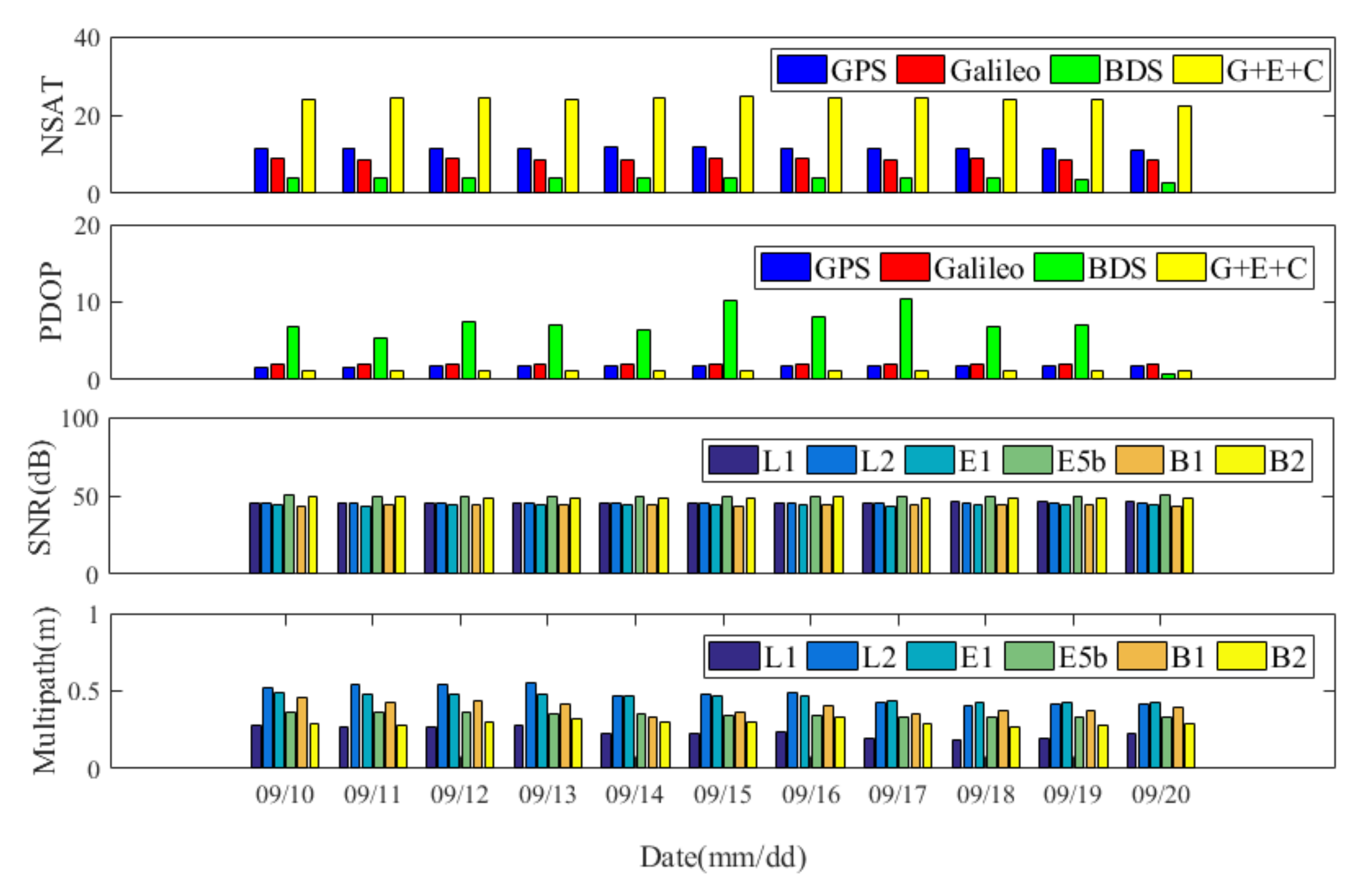
The quality of satellite signals can greatly affect positioning accuracy. However, little work has been performed to analyze GNSS signal quality in the Arctic NEP. To address this issue, we first discuss the corresponding quality metrics, including the maximum satellite elevation, NSAT, PDOP, SNR, and multipath errors.

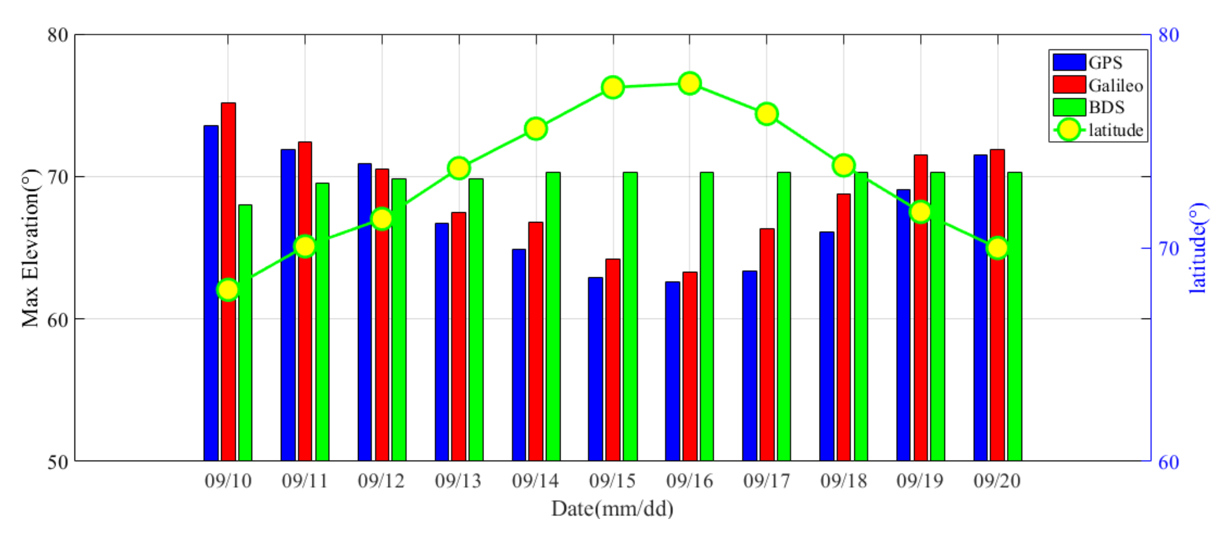
Both tropospheric and ionospheric errors have considerable impacts on GNSS positioning, and lower altitudes usually result in larger atmospheric and multipath errors. In addition, the satellite elevation angle at high latitudes is usually low; thus, it is necessary to discuss the satellite elevation in the NEP.

The NSAT and the DOP represent certain spatial geometry features of GNSS satellites. The PDOP reflects positional geometry in the X, Y, and Z directions [20], which can be calculated as below:

$$\begin{array}{c}\hfill \delta P_m=Bdx+e_{m}d{t}_r+e_p\end{array}$$

(1)

where the vector of $\delta P_m$ denotes the observed pseudo–range minus computed values; B denotes the corresponding design matrix; and $d{t}_r$ is the estimated receiver clock offset. $e_m$ is the m–th row vector with all unit values of 1. The vector of $e_p$ denotes the pseudo–range observation noises.

$$\begin{array}{c}\hfill A={\left(B^{T}B\right)}^{-1}=\left\{\begin{array}{ccc}{A}_{11}& A_{12}& A_{13}\\ A_{21}& A_{22}& A_{23}\\ A_{31}& A_{31}& A_{33}\end{array}\right\}\end{array}$$

(2)

$$\begin{array}{c}\hfill PDOP=\sqrt{A_{11}+A_{22}+A_{33}}\end{array}$$

(3)

The receiver SNR is related to factors such as residual atmospheric and multipath errors, antenna gains, and the internal circuit design of the receiver, which reflects the data quality and the observation noise level.

The signal received by the GNSS receiver includes not only the direct signal, but also the reflected signal from nearby objects (such as the sea surface); thus, multipath errors should be considered due to the interference of these two signals. The multipath error $M{P}_{r,j1}^s$ of the $j1$ signal can be approximated as [21]:

$$\begin{array}{c}\hfill M{P}_{r,j1}^s=P_{r,j1}^s-\frac{f_{r,j1}^s+f_{r,j2}^s}{f_{r,j1}^s-f_{r,j2}^s}{\lambda }_{j1}{\phi }_{r,j1}^s+\frac{2f_{r,j1}^s}{f_{r,j1}^s-f_{r,j2}^s}{\lambda }_{j2}{\phi }_{r,j2}^s-B_{r,j1}^s\end{array}$$

(4)

$$\begin{array}{c}\hfill B_{r,j1}^s=\frac{f_{r,j1}^s+f_{r,j2}^s}{f_{r,j1}^s-f_{r,j2}^s}{\lambda }_{j1}{N}_{r,j1}^s+\frac{2f_{r,j1}^s}{f_{r,j1}^s-f_{r,j2}^s}{\lambda }_{j2}{N}_{r,j2}^s+d_{r,j1}-d_{j1}^s\end{array}$$

(5)

where s, r, and $j(j1,j2)$ denote the satellite PRN (pseudo random noise), receiver, and carrier frequency; $P_{r,j1}^s$ and ${\phi }_{r,j1}^s$ are the pseudo–range and carrier–phase observation, respectively; $d_{r,j1}$ and $d_{j1}^s$ are the code biases; ${\lambda }_j$ is the wave–length, and $f_{r,j}^s$ is the frequency.

2.2. GNSS Real–Time PPP Model

2.2.1. Multi–GNSS SF RT–PPP Model

The standard uncombined single–frequency PPP model can be expressed as follows:

$$\begin{array}{c}\hfill \left\{\begin{array}{c}{L}_{r,j}^{sys,s}={\rho }_r^{sys,s}+c\left(d{t}_r^{sys}-d{t}^{sys,s}\right)+{\lambda }_j^{sys}\left(b_{r,j}^{sys}-b_j^{sys,s}\right)+{\lambda }_j^{sys}{N}_{r,j}^{sys,s}-I_{r,j}^{sys,s}+T_r^{sys,s}+{\epsilon }_{r,j}^{sys,s}\hfill \\ P_{r,j}^{sys,s}={\rho }_r^{sys,s}+c\left(d{t}_r^{sys}-d{t}^{sys,s}\right)+d_{r,j}^{sys}-d_j^{sys,s}+I_{r,j}^{sys,s}+T_r^{sys,s}+e_{r,j}^{sys,s}\hfill \end{array}\right.\end{array}$$

(6)

where L and P are the carrier phase and pseudo–range observation, respectively; $sys$ represents the GNSS system; ${\rho }_r^s$ is the satellite–receiver geometric distance; $d{t}_r$ and $d{t}^s$ represent the clock bias; ${\lambda }_j$ is the wavelength of frequency j; b and d are the phase delay and the code biases; N is the integer ambiguity; $I_{r,j}^s$ is the ionospheric delay at frequency j; $T_r^s$ is the tropospheric delay; and $e_{r,j}^s$ and ${\epsilon }_{r,j}^s$ denote the pseudo–range and carrier phase observation noise.

2.2.2. Multi–GNSS Ionospheric–Free (IF) DF RT–PPP Model

The ionosphere is a dissipative medium; thus, the ionospheric errors of GNSS signals are frequency dependent, which can be expressed as:

$$\begin{array}{c}\hfill I_{r,j}^{sys,s}=k_j{I}_{r,1}^{sys,s},k_j=\frac{f_1^{sys}}{f_j^{sys}}\end{array}$$

(7)

Therefore, the linear combination (LC) of GNSS observations at different frequencies can effectively eliminate the influence of the first–order ionosphere errors,

$$\begin{array}{c}\hfill \left\{\begin{array}{c}{L}_{r,IF}^{sys,s}=\alpha L_{r,1}^{sys,s}+\beta L_{r,2}^{sys,s}\hfill \\ P_{r,IF}^{sys,s}=\alpha L_{r,1}^{sys,s}+\beta L_{r,2}^{sys,s}\hfill \end{array}\right.,\alpha =\frac{f_1^{sy{s}^2}}{f_1^{sy{s}^2}-f_2^{sy{s}^2}},\beta =-\frac{f_2^{sy{s}^2}}{f_1^{sy{s}^2}-f_2^{sy{s}^2}}\end{array}$$

(8)

Then, the undifferentiated IF–LC RT–PPP model can be expressed [22]:

$$\begin{array}{c}\hfill \left\{\begin{array}{c}{L}_{r,IF}^{sys,s}={\rho }_r^{sys,s}+c\left(d{t}_r^{sys}-d{t}^{sys,s}\right)+{\lambda }_{IF}^{sys}\left(b_{r,IF}^{sys}-b_{IF}^{sys,s}\right)+{\lambda }_{IF}^{sys}{N}_{r,IF}^{sys,s}+T_r^{sys,s}+{\epsilon }_{r,IF}^{sys,s}\hfill \\ P_{r,IF}^{sys,s}={\rho }_r^{sys,s}+c\left(d{t}_r^{sys}-d{t}^{sys,s}\right)+d_{r,IF}^{sys}-d_{IF}^{sys,s}+T_r^{sys,s}+e_{r,IF}^{sys,s}\hfill \end{array}\right.\end{array}$$

(9)

To ensure the calculation efficiency, as well as the product accuracy, IGS and some of the ACs use the IF–LC model in real–time precise ephemeris and clock calculation. As a result, the receiver and the satellite code biases $d_{r,IF}$ and $d_{IF}^{sys,s}$ will be absorbed by the receiver and satellite clock, respectively. Meanwhile, the phase delays $b_{r,IF}^{sys}$ and $b_{IF}^{sys,s}$ will be absorbed by phase ambiguities. Therefore, Equation (9) can be rewritten as:

$$\begin{array}{c}\hfill \left\{\begin{array}{c}{L}_{r,IF}^{sys,s}={\rho }_r^{sys,s}+c\left(d{\widehat{t}}_r^{sys}-d{\widehat{t}}^{sys,s}\right)+{\lambda }_{IF}^{sys}{\widehat{N}}_{r,IF}^{sys,s}+T_r^{sys,s}+{\epsilon }_{r,IF}^{sys,s}\hfill \\ P_{r,IF}^{sys,s}={\rho }_r^{sys,s}+c\left(d{\widehat{t}}_r^{sys}-d{\widehat{t}}^{sys,s}\right)+T_r^{sys,s}+e_{r,IF}^{sys,s}\hfill \end{array}\right.\end{array}$$

(10)

with

$$\begin{array}{c}\hfill \left\{\begin{array}{c}cd{\widehat{t}}_r^{sys}=cd{t}_r^{sys}+d_{r,IF}^{sys}\hfill \\ cd{\widehat{t}}^{sys,s}=cd{t}^{sys,s}+d_{IF}^{sys,s}\hfill \\ {\widehat{N}}_{r,IF}^{sys,s}=N_{r,IF}^{sys,s}+\left(b_{r,IF}^{sys}-b_{IF}^{sys,s}\right)+\frac{1}{{\lambda }_{IF}^{sys}}\left(d{t}_r^{sys}-d{t}^{sys,s}\right)\hfill \end{array}\right.\end{array}$$

(11)

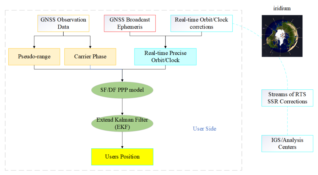
2.2.3. RT–PPP Method in NEP

We processed the RT–PPP method in the NEP in three steps, i.e., data collection, real–time precise orbit/clock calculation, and PPP processing. In the first step, we received data including GNSS observation data, broadcast ephemeris, and real–time orbit/clock corrections via LEO, such as Iridium. In the second step, we calculated the real–time precise orbit and clock by using the real–time orbit/clock corrections, and the specific calculation process referred to in (https://igs.org/wg/real-time, accessed on 1 February 2022). In the third step, we used the PPP model mentioned above and an extended Kalman filter to obtain the users’ positions. The specific RT–PPP method in the NEP is shown in Figure 1.

2.3. GNSS Data Collection in NEP

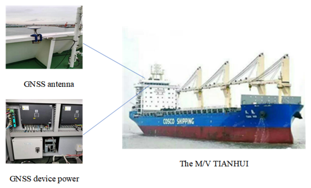
We installed a data acquisition system on the M/V TIANHUI, including a low–cost U–blox ZED–F9P GNSS receiver and a GNSS antenna, to evaluate the RT–PPP positioning performance in the NEP. Figure 2 shows that TIANHUI is a cargo ship with a length of 190 m and a width of 29 m. The GNSS antenna is placed on the ship deck, and the power supply and receiver are installed in the cabin equipment room.

The M/V TIANHUI set sail from Yangshan Port in Shanghai on 30 August 2019, crossed the Bering Strait into the NEP on 10 September, and entered the Norwegian Sea on 20 September, which is shown in Figure 3. The total voyage on the NEP was approximately 3000 nautical miles, and we collected approximately 11 days of GNSS raw observation data with a 1 s sampling rate. However, the GLONASS signal was shielded in the data acquisition process; as such, we only collected GPS, Galileo, and BDS observation data.

Meanwhile, we received the CLK93 stream of the state–space representation (SSR) orbit/clock correction products, which contain the correction information for Multi–GNSS, via NTRIP Caster by BNC software, and the data period was from 10 September to 20 September 2019.

3. Results

3.1. GNSS Signal Quality in NEP

Satellite signal quality is closely related to positioning accuracy, therefore, we analyzed the maximum satellite elevations, NSAT, PDOP, SNR, and multipath errors of GPS, Galileo, and BDS.

GNSS uses a specific orbital inclination to cover densely populated mid– and low–latitude areas, which means that the satellite elevation angle will be lower when sailing in polar regions [5]. Consequently, this may produce poor satellite geometry. Furthermore, the complex environment in the polar region may affect the GNSS signal and positioning accuracy. Therefore, herein, we analyze the spatial structures and signal quality of GPS, Galileo, and BDS–2 (because CLK93 products only provided BDS–2 correction information).

Figure 4 shows the variation between the maximum satellite elevation in a day and the ship’s average latitude in the NEP. The maximum GPS and Galileo satellite elevations vary considerably with latitude. The maximum GPS and Galileo satellite elevations are approximately 75° when the latitude of the ship is approximately 68° N, while they are 60° when the ship reaches 78° N. Conversely, the maximum BDS satellite elevation is not sensitive to latitude changes in the NEP, which remains at approximately 65°–70° because of the contributions of inclined geo–synchronous orbit (IGSO) BDS satellites. Although they have the same orbital inclinations as medium–Earth–orbit (MEO) satellites, their orbital altitudes are about twice as much.

Figure 5 shows the variation between the GNSSs’ NSAT and the ship position in the NEP. We found that the NSAT did not significantly decrease when the ship entered high latitudes (approximately 78° N). There are more than 10 and 7 satellites that can be observed for GPS and Galileo, respectively, most of the time, while the BDS has less than 4. After the combination, the NSAT remained above 16.

Figure 6 further illustrates the availability of GNSS in the NEP, and shows the one–day average NSAT, PDOP, SNR, and multipath errors for GPS, Galileo, and BDS.

Table 1. Mean values of NSAT and PDOP for GPS, Galileo, BDS, and multi–GNSS (G+E+C) from 10 September to 20 September 2019.

	GPS	Galileo	BDS	G+E+C
NSAT	11.556	8.729	3.766	24.050
PDOP	1.753	2.009	6.940	1.113

summarizes the 11–day mean values of NSAT and PDOP for GPS, Galileo, BDS, and multi–GNSS from 10 September to 20 September 2019, and

Table 2. Mean SNR and multipath errors of each GNSS signal from 10 September to 20 September 2019.

System	GPS		Galileo		BDS
Frequency	L1	L2	E1	E5b	B1	B2
SNR (dB)	45.769	45.158	43.946	49.897	43.966	48.744
Multipath (m)	0.234	0.478	0.458	0.348	0.394	0.295

shows the average SNR and multipath errors of each GNSS signal in the NEP.

Figure 6 shows the NSAT is inversely proportional to the PDOP. The NSAT of BDS is the least proportional, with an average of 3.766, because BDS–2 is a regional satellite navigation system that mainly covers the Asia–Pacific region. While GPS and Galileo have more satellites than BDS (11.556 and 8.729, respectively), their PDOP values are relatively stable. Moreover, the sum number of satellites in all systems can reach approximately 24.050, and the multi–GNSS PDOP value is 1.113. For the SNR, we found that the change of daily–average SNR values is not significant, and there is a slight gap between the different frequencies. Galileo E5b has the highest SNR (49.897 dB); however, Galileo E1’s SNR is the lowest (43.946 dB). The GPS L1 and L2 SNR values are approximately equal (45.769 dB and 45.158 dB, respectively). The SNR value of the BDS B2 signal is higher than that of the B1 signal, and the mean values are 48.744 dB and 43.966 dB, respectively. For multipath errors, one can notice that it considerably changes with environment variation. In general, the GPS L1 signal has the strongest ability to resist multipath interference, which is about two times better than that of the GPS L2, Galileo E1, and BDS B1 signals, and approximately 1.5 times better than that of the Galileo E5b signal.

3.2. RT–PPP Performance in NEP

3.2.1. Performance of Real–Time CLK93 Products

For RT–PPP, the positioning performance is highly related to the quality of real–time SSR corrections. Therefore, we took GFZ GBM products as references to evaluate the CLK93 SSR product. Additionally, we used BKG NTRIP Client (BNC) software to receive the CLK93 stream, and collected data with 5 s intervals from 10 to 20 September 2019.

First, we evaluated the real–time orbit accuracy of GPS, GLONASS, Galileo, and BDS corrected by CLK93 SSR products. Figure 7 illustrates the 11–day average RMS values of orbit in X/Y/Z components, as well as in a three–dimensional (3D) direction. For GPS, we can see that almost all satellite accuracies are better than 0.05 m, while they are better than 0.08 m in 3D except the PRN G09, which has a significant error (worse than 0.15 m in the X/Y/Z directions, and 0.25 m in 3D). For GLONASS, the orbit accuracy is generally between 0.03 and 0.08 m in the X/Y/Z directions and approximately 0.1 m in 3D; however, the orbital error of the PRN R01 satellite is relatively large, and its 3D accuracy is approximately 0.21 m. Galileo has the highest satellite accuracy in the X/Y/Z directions (better than 0.05 m), while in 3D, it is better than 0.08 m. For BDS satellites, we excluded GEO satellites (PRN C01 to C05) due to their poor accuracy (lower than 1 m); furthermore, their real–time orbit is better than 0.10 m in the X/Y/Z directions, and between 0.08 and 0.16 m in the 3D direction, except for the PRN C06 satellite.

Table 3. Eleven–day mean RMS values of CLK93 products’ orbits.

	X (m)	Y (m)	Z (m)	3D (m)
GPS	0.039	0.038	0.032	0.063
GLONASS	0.052	0.051	0.055	0.092
Galileo	0.034	0.031	0.033	0.056
BDS	0.087	0.082	0.076	0.142

shows the mean RMS values of the four GNSSs’ corrected orbits. Galileo has the highest orbit accuracy, and its 3D RMS is 0.052 m. The GPS orbital accuracy, which is 0.063 m, is a bit lower than Galileo’s. The RMS of the GLONASS is 0.092 m, which ranks third. As for the BDS, the mean RMS of the 3D orbit is 0.142 m, which is three times worse than Galileo.

Similarly, we analyzed the real–time clock errors corrected by CLK93 products. When comparing different IGS clock products, it is necessary to select a reference satellite in each GNSS to eliminate systematic biases [23]. For this reason, we selected GPS G32, GLONASS R24, Galileo E36, and BDS C14 satellites in each system. We computed both the standard deviation (STD) and RMS of each satellite clock to reflect the accuracy and consistency of clock biases.

Figure 8 shows the STD and RMS of each satellite clock, and the mean values are displayed in

Table 4. Eleven–day mean STD and RMS values of CLK93 products’ clocks.

	STD (ns)	RMS (ns)
GPS	0.130	0.332
GLONASS	0.623	3.622
Galileo	0.084	0.254
BDS	0.346	0.802

. Regarding the STD, the Galileo clock has the highest accuracy and considerable stability; furthermore, all satellite clock STDs are better than 0.15 ns, and the average value is 0.084 ns (approximately 2.5 cm). The accuracy of the GPS clock is slightly lower than that of Galileo, the STD values are better than 0.3 ns except for G09, and the mean value is 0.13 ns (approximately 4.0 cm). Compared with the GPS and Galileo clock, the accuracy of the real–time clock error of the BDS satellite is considerably lower, and its average STD is 0.346 ns (approximately 10.0 cm). The precision of the GLONASS clock is the lowest, with all satellite clock STDs worse than 0.3 ns, and the mean value is 0.623 ns (approximately 18.0 cm). Regarding the RMS, the Galileo clock still has the smallest RMS value at 0.254 ns. However, the RMS value of the GLONASS clock is the largest, indicating an inferior consistency in the GLONASS clock biases.

3.2.2. Performance of SF RT–PPP in the NEP

Although multi–GNSS data can be collected by low–cost receivers, some of them can only obtain the single–frequency data of a certain system. Therefore, we took an SF RT–PPP model into account to evaluate performance in the Arctic regions.

Table 5. SF RT–PPP data processing strategy.

Items	Models/Strategies
Satellites	GPS/GPS+Galileo+BDS
Observations	Uncombined code and carrier–phase measurements
Sampling rate	1 s
Elevation cutoff	10°
Observation weight	Elevation–dependent weight; GPS:Galileo:BDS = 1:1:2
Precise products	CLK93 real–time stream from CNES
Satellite antenna phase center	igs14.atx
Phase–windup effect	Corrected [24]
Ionospheric delay	Klobuchar model
Tropospheric delay	GPT2 + GMF
Tide effects	Solid Earth + pole + ocean tide
Phase ambiguities	Real value

summarizes the multi–GNSS SF RT–PPP data processing strategies.

We used the data collected by the M/V TIANHUI from 10:00 to 22:00 on 12 September 2019 to evaluate the positioning performance of SF RT–PPP in the NEP. We analyzed single–GPS and multi–GNSS combinations of SF RT–PPP performance in this section. Due to the lack of reference base stations in polar regions, we obtained the reference solutions by post–processing PPP based on GBM products. Figure 9a,b show the position errors in the east, north, and up components, as well as the NSAT and PDOP values of GPS and multi–GNSS. In the east direction, both the GPS and multi–GNSS of the SF RT–PPP can achieve meter–level positioning accuracy, and the combined precision is slightly higher than that of GPS. However, we observed large fluctuations for GPS in the north and up directions, and the errors are even greater than 10 m in the north. Moreover, multi–GNSS is more stable and meter–level accuracy can be realized in each direction because the number of combined GNSSs are twice that of GPS, and they also have a better satellite space structure. Although GPS always has six or more satellites, the PDOP values are occasionally larger and show more variations than the multi–GNSS.

Figure 10 illustrates the 11–day RMS values of SF RT–PPP positioning results in the east, north, horizontal, up, and 3D components. The GPS SF RT–PPP solution is shown in blue while the combined solution is in red. The positioning accuracy of the north component is lower than that of the east. In addition, the accuracy in the north is roughly equivalent to that in the vertical direction, resulting in a lower horizontal precision. This phenomenon is due to the poor north–south structure of the GNSS satellites in the NEP.

Table 6. Mean RMS values of SF RT–PPP performance in the east, north, 2D, up, and 3D directions for GPS and multi–GNSS from 10 to 20 September 2019.

	E (m)	N (m)	2D (m)	U (m)	3D (m)
GPS	1.956	4.048	4.869	4.609	7.268
G+E+C	1.553	2.931	3.596	3.110	5.138

shows the mean RMS values in each direction of SF RT–PPP in the NEP. In general, the accuracy of SF RT–PPP is significantly improved by using multi–GNSS—an increase of approximately 29.3% in 3D, from 7.268 m to 5.138 m. In the east and north coordinates, 20.6% and 27.0% improvements are achieved, revealing an improvement of approximately 26.0% in the horizontal component after the combination. Moreover, the vertical direction shows an improvement of approximately 32.5%.

3.2.3. Performance of DF RT–PPP in the NEP

Because the U–blox F9P can receive GPS, Galileo, and BDS dual–frequency signals, we used a DF RT–PPP model to further verify the performance of RT–PPP in the NEP. However, some GPS satellites, such as G02, G11, G16, G19, and G20, only contain single–frequency data because the carrier phase on L2 is derived from the mixed channel in the U–blox F9P receiver (https://igs.org/formats-and-standards/, accessed on 1 February 2022). We used the IF–LC code and carrier–phase observations in the DF RT–PPP model. Furthermore, we used GPS L1/L2, Galileo E1/E5a, and BDS–2 B1/B2 dual–frequency signals. Moreover, our other strategies are similar to those in Table 5.

Figure 11a illustrates east/north/up coordinates with DF RT–PPP solutions for GPS and multi–GNSS from 10:00 to 22:00 on 12 September 2019, and Figure 11b shows the NSAT and PDOP values. Figure 11a shows that both GPS and multi–GNSS can achieve decimeter– and centimeter–level accuracy after convergence. However, it takes a long time for GPS to converge, and it often diverges after convergence. Figure 11b shows that large PDOP values are highly consistent with the divergence for GPS RT–PPP positioning results. Furthermore, the number of GPS satellites decreased considerably compared with the SF RT–PPP because dual–frequency cannot be observed by some GPS satellites. Conversely, the multi–GNSS RT–PPP solution tends to be more stable because of the increased number of satellites and a more stable spatial structure than the single GPS.

Figure 12 represents the daily RMS values in each of the five components for the GPS and GPS/Galileo/BDS combinations during the 11–day testing period when the M/V TIANHUI passed through the NEP. The GPS RT–PPP solution is shown in blue, while the combination solution is shown in red. The GPS can only achieve decimeter–level positioning accuracy in the horizontal and up directions, and sub–meter–level accuracy in the 3D direction because of the small number of GPS satellites. However, sub–decimeter or centimeter accuracy can be realized after the combination of GPS, Galileo, and BDS in each direction.

Table 7. Mean RMS values of DF RT–PPP performance in the east, north, horizontal, up, and 3D directions for GPS and multi–GNSS from 10 September to 20 September 2019.

	E (m)	N (m)	2D (m)	U (m)	3D (m)
GPS	0.153	0.223	0.300	0.257	0.434
G+E+C	0.043	0.058	0.080	0.057	0.107

summarizes the average RMS values in each direction. The accuracy of the north direction is still slightly lower than that of the east in the DF RT–PPP model. The combined results are improved by 73.3% in the horizontal direction compared with single GPS. In terms of the up direction, the positioning accuracy changes from 0.257 m to 0.057 m, and an improvement of approximately 77.8% is achieved when performing the combination DF RT–PPP model. Concerning the 3D component, the accuracy is of approximately 0.434 m for GPS DF RT–PPP, while 0.107 m is achieved by the combination, indicating an improvement of approximately 75.3%.

4. Discussion

Ionospheric refraction error is one of the main error sources in GNSS positioning, and the first–order ionospheric term can reach several meters or even tens of meters because it is frequency dependent and can be eliminated using an IF–LC model at different frequencies [25,26].

However, for the SF PPP, ionospheric models need to be used for correcting ionospheric propagation errors. In Section 3.2.2, we used the Klobuchar model [27] because it is simple and parameters can be obtained in the broadcast ephemerides; therefore, we can calculate the ionospheric propagation errors in real time. However, this model only offers 50–75% accuracy for ionospheric corrections, and the accuracy is lower at high latitudes [28]. The IGS developed and published RTCM–SSR messages for vertical total–electron–content (VTEC) ionospheric messages in October 2020 [29], which means that the grid ionospheric model (GIM) information will be released in real time, effectively improving the positioning accuracy of single–frequency receiver users in the NEP.

However, IGS does not provide real–time GIM products in SSR formats; therefore, we used the post–processing GIM products provided by the Chinese Academy of Sciences [30] to simulate real–time VTEC ionospheric messages.

After obtaining the ionospheric grid file, the interpolation method can be used to obtain the TEC values at time t:

$$\begin{array}{c}\hfill TEC\left({\lambda }_{IPP},{\phi }_{IPP},t\right)=\frac{T_{i+1}-t}{T_{i+1}-T_i}TE{C}_i\left({\lambda }_{IPP},{\phi }_{IPP}\right)+\frac{t-T_i}{T_{i+1}-T_i}TE{C}_{i+1}\left({\lambda }_{IPP},{\phi }_{IPP}\right)\end{array}$$

(12)

where ${\lambda }_{IPP}$ and ${\phi }_{IPP}$ are the longitude and latitude of the satellite signal ionospheric pierce point (IPP), and $TE{C}_i$ and $TE{C}_{i+1}$ are the provided TEC data at time $T_i$ and $T_{i+1}$. Then, the vertical ionospheric delay $I_v$ can be calculated as follows:

$$\begin{array}{c}\hfill I_v=-\frac{40.3}{f^2}TEC\left({\lambda }_{IPP},{\phi }_{IPP},t\right)\end{array}$$

(13)

Finally, the slant ionospheric delay I can be expressed as:

$$\begin{array}{c}\hfill I=\frac{1}{z^{\prime }}{I}_v\end{array}$$

(14)

where $z^{\prime }$ is the zenith at IPP. Substituting Equation (14) into the SF–PPP model (Equation (1)), the user’s real–time coordinates can be obtained.

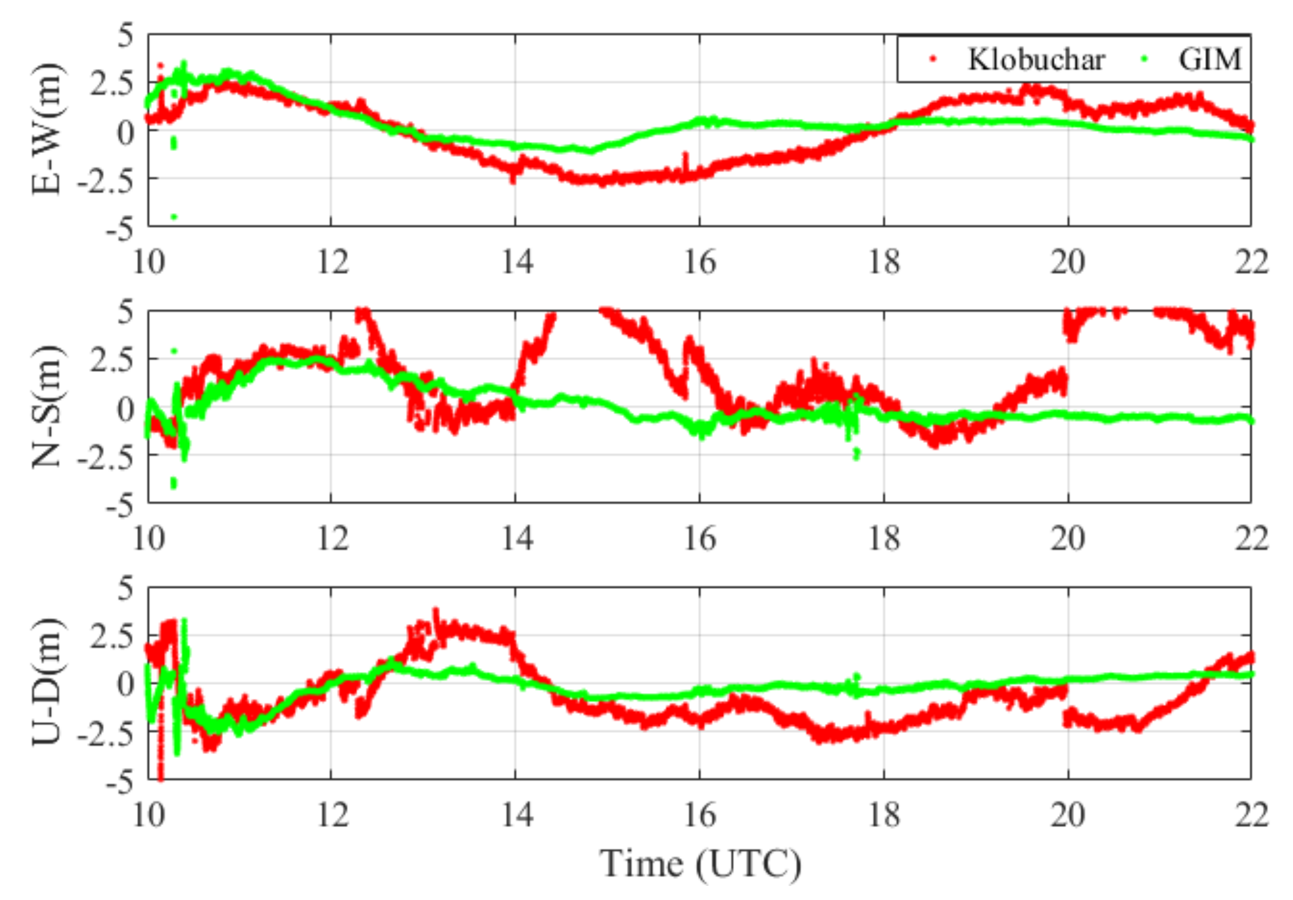
We performed the two aforementioned SF RT–PPP scenarios, including the Klobuchar– and GIM–based models, to examine and compare the effectiveness of ionospheric products. Figure 13 shows the east/north/up–coordinate solutions of the two scenarios utilizing the GPS/Galileo/BDS combination from 10:00 to 22:00 on 12 September 2019, while the GIM– and Klobuchar–based SF RT–PPP models are shown in green and red, respectively. We determined that the positioning accuracy can be considerably improved by using GIM products, especially in the north component.

Table 8. RMS values of Klobuchar–based and GIM–based SF RT–PPP solutions in the east, north, horizontal, up, and 3D directions from 10:00 to 22:00 on 12 September 2019.

	E (m)	N (m)	2D (m)	U (m)	3D (m)
Klobuchar	1.925	3.917	4.365	2.630	5.096
GIM	1.056	0.978	1.440	0.863	1.679

summarizes the RMS values in each direction of the two aforementioned SF RT–PPP methods. Compared with the accuracy of 4.365 m and 2.630 m for the horizontal and vertical components derived from Klobuchar–based RT–PPP solutions, the results of the GIM–based solutions show improvements of 1.440 m and 0.863 m, which is approximately 67.0% and 67.2%. The positioning accuracy for the 3D component improves from 5.096 m with the Klobuchar–based solutions to 1.649 m with the GIM–based solutions—an improvement of 66.7%.

In conclusion, if the real–time IGS ionospheric products are used, single–frequency receiver users will be able to achieve 1–meter–level or higher positioning accuracy in the NEP.

5. Conclusions

GNSS is one of the most widely used positioning methods in the Arctic regions. The main algorithm used in the polar regions is GNSS single–point positioning (SPP); however, its meter–level positioning accuracy is poor. Furthermore, its precision cannot meet the requirements of some Arctic projects, e.g., precise oil drilling. Precise point positioning (PPP) can achieve sub–decimeter and centimeter–level positioning accuracy using one GNSS receiver. Some scholars have researched PPP algorithms in the polar regions; however, it still cannot meet the requirements of real–time positioning due to the several–day latency of the precise ephemeris. Few scholars have studied RT–PPP because of its lack of reliable communication links. Nevertheless, real–time services provided by IGS and easy–access satellite communication systems available in the NEP have opened the opportunity for precise multi–GNSS products in real–time. Therefore, in our paper, we analyzed the use of RT–PPP in the Arctic NEP.

We evaluated the positioning performance of RT–PPP in the NEP during the period between 10 September and 20 September 2019. Moreover, we collected our GNSS data using a U–blox F9P receiver installed on the M/V TIANHUI.

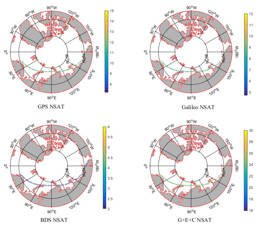
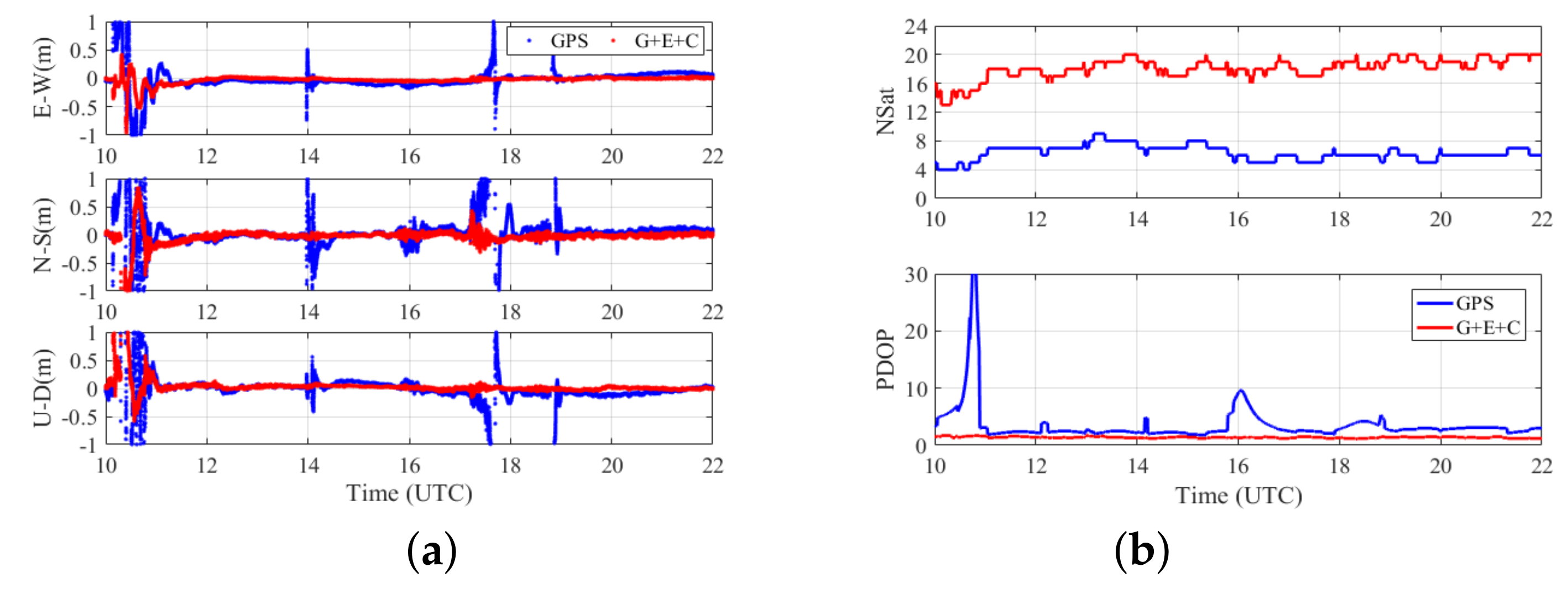
We also evaluated the satellite signal quality. Our results show that the maximum satellite evaluations vary considerably with latitude for GPS and Galileo, while BDS is less sensitive to latitude changes due to the contribution of BDS IGSO. PDOP is usually inversely proportional to NSAT, reflecting the quality of the satellite structure. We found that the NSAT for GPS and Galileo is larger than that of BDS; as a result, PDOP for GPS and Galileo is lower and more stable. Moreover, the above three systems have a total of 24 satellites that yield the smallest PDOP values. We also observed consistent daily SNR values prone to environmental changes. On the other hand, multipath errors showed large variations over different bands, as well as environmental changes, where the differences sometimes reached the decimeter level.

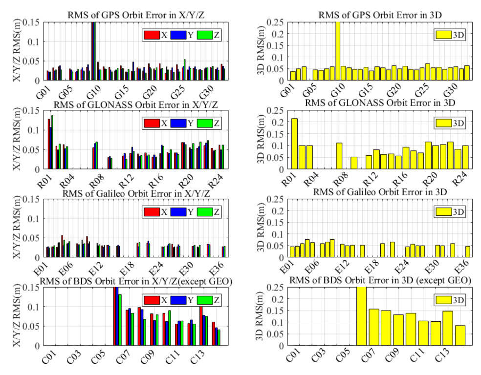
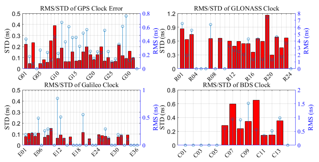
In addition to the satellite signal quality, the real–time SSR corrections also affected the positioning performance. We used CLK93 products, which include multi–GNSS correction information, and investigated their performance over an 11–day testing period. Our results show that Galileo has the best performance, both in satellite orbit and clock, which are approximately 0.056 m in 3D and 0.084 ns, respectively. GPS shows comparable performance to Galileo, with 0.063 m in the 3D component and 0.130 ns for the real–time clock. BDS and GLONASS show some disadvantages, with BDS exhibiting the lowest orbit accuracy of 0.142 m, while GLONASS yielded the worst satellite clock of 0.623 ns.

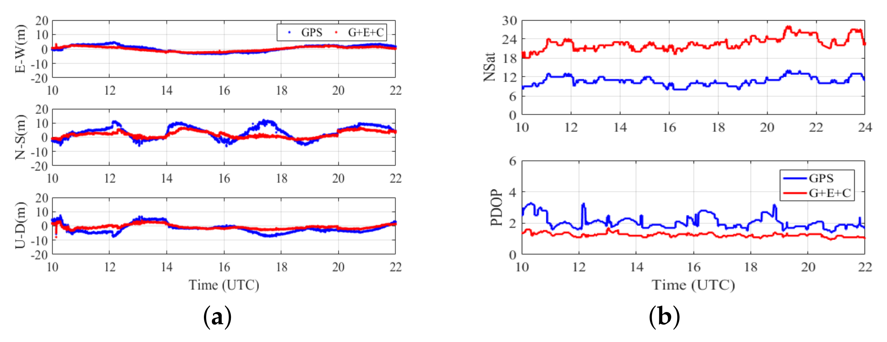
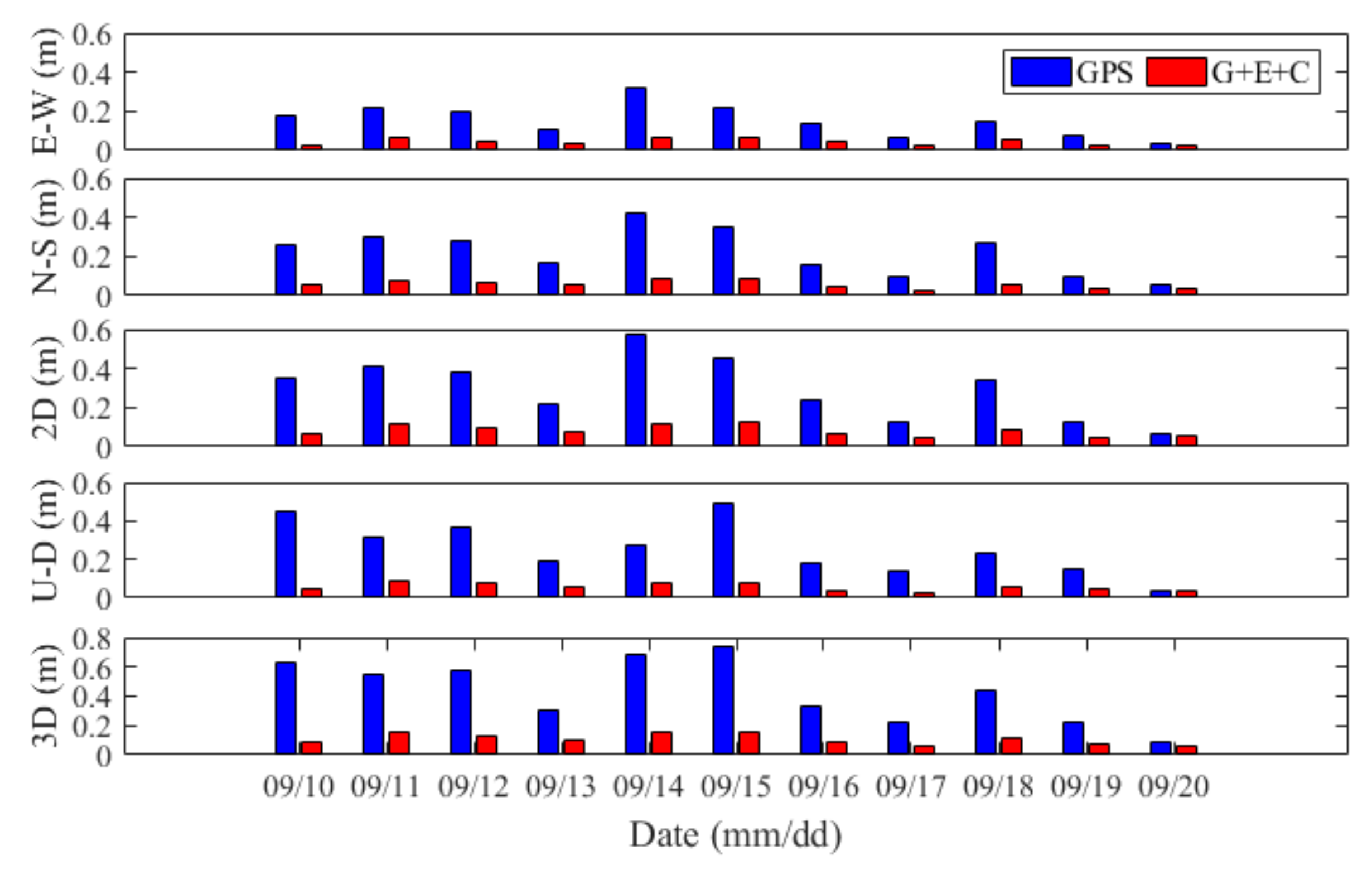
As for the RT–PPP performance in the NEP, 1–meter–level positioning accuracy can be achieved with GIM–based SF RT–PPP, while the DF RT–PPP model reaches a sub–decimeter and centimeter–level accuracy. With a multi–GNSS combination, we can further improve the precision of the RT–PPP for both SF and DF models. Furthermore, with multi–GNSS, the average RMS value in the horizontal(vertical) direction is 0.080(0.057) m, a 70% improvement over single–GPS solutions. However, due to the complexity of the marine environment, fault observation data may appear. Therefore, we will carry out more effective fault detection in our future research to further improve the reliability of RT–PPP in the Arctic region [31,32].

References

1. Cassano, J.J.; DuVivier, A.; Roberts, A.; Hughes, M.; Seefeldt, M.; Brunke, M.; Craig, A.; Fisel, B.; Gutowski, W.; Hamman, J.; et al. Development of the Regional Arctic System Model (RASM): Near-surface atmospheric climate sensitivity. J. Clim. 2017, 30, 5729–5753. [Google Scholar] [CrossRef]
2. Wang, M.; Overland, J.E. A sea ice free summer Arctic within 30 years: An update from CMIP5 models. Geophys. Res. Lett. 2012, 39. [Google Scholar] [CrossRef]
3. Buixadé Farré, A.; Stephenson, S.R.; Chen, L.; Czub, M.; Dai, Y.; Demchev, D.; Efimov, Y.; Graczyk, P.; Grythe, H.; Keil, K.; et al. Commercial Arctic shipping through the Northeast Passage: Routes, resources, governance, technology, and infrastructure. Polar Geogr. 2014, 37, 298–324. [Google Scholar] [CrossRef]
4. An, L.; Ma, L.; Wang, H.; Zhang, H.Y.; Li, Z.H. Research on navigation risk of the Arctic Northeast Passage based on POLARIS. J. Navig. 2022, 75, 455–475. [Google Scholar] [CrossRef]
5. Zhang, Q.; Chen, Z.; Cui, Y.; Zheng, X.; Rong, F.; Sun, Y.; Gao, L. A refined metric for multi-GNSS constellation availability assessment in polar regions. Adv. Space Res. 2020, 66, 655–670. [Google Scholar] [CrossRef]
6. Huang, W.; Fang, T.; Luo, L.; Zhao, L.; Che, F. A damping grid strapdown inertial navigation system based on a Kalman filter for ships in polar regions. Sensors 2017, 17, 1551. [Google Scholar] [CrossRef]
7. Yang, Y.; Xu, J. Navigation performance of BeiDou in polar area. Geomat. Inf. Sci. Wuhan Univ. 2016, 41, 15–20. [Google Scholar]
8. Li, X.; Ge, M.; Dai, X.; Ren, X.; Fritsche, M.; Wickert, J.; Schuh, H. Accuracy and reliability of multi-GNSS real-time precise positioning: GPS, GLONASS, BeiDou, and Galileo. J. Geod. 2015, 89, 607–635. [Google Scholar] [CrossRef]
9. Leppälä, L.; Honkala, S.; Ferrara, G.; Kirkko-Jaakkola, M.; Kuusniemi, H.; Miettinen-Bellevergue, S. Challenges in Arctic navigation: The user perspective. In Proceedings of the 2019 European Navigation Conference (ENC), IEEE, Warsaw, Poland, 9–12 April 2019; pp. 1–8. [Google Scholar]
10. Kouba, J.; Héroux, P. Precise point positioning using IGS orbit and clock products. GPS Solut. 2001, 5, 12–28. [Google Scholar] [CrossRef]
11. Zumberge, J.; Heflin, M.; Jefferson, D.; Watkins, M.; Webb, F. Precise point positioning for the efficient and robust analysis of GPS data from large networks. J. Geophys. Res.-Solid Earth 1997, 102, 5005–5017. [Google Scholar] [CrossRef]
12. Zhang, X.; Andersen, O.B. Surface ice flow velocity and tide retrieval of the Amery ice shelf using precise point positioning. J. Geod. 2006, 80, 171–176. [Google Scholar] [CrossRef]
13. Yao, X.; Chen, M.; Zuo, Z.; Wang, J. Performance analysis on polar BDS PPP. J. Navig. Position. 2018, 6, 57–63. [Google Scholar]
14. Dabove, P.; Linty, N.; Dovis, F. Analysis of multi-constellation GNSS PPP solutions under phase scintillations at high latitudes. Appl. Geomat. 2020, 12, 45–52. [Google Scholar] [CrossRef]
15. Di, M.; Zhang, A.; Guo, B.; Zhang, J.; Liu, R.; Li, M. Evaluation of Real-Time PPP-Based Tide Measurement Using IGS Real-Time Service. Sensors 2020, 20, 2968. [Google Scholar] [CrossRef] [PubMed]
16. Guo, B.; Di, M.; Song, F.; Li, J.; Shi, S.; Limsupavanich, N. Integrated coseismic displacement derived from high-rate GPS and strong-motion seismograph: Application to the 2017 Ms 7.0 Jiuzhaigou Earthquake. Measurement 2021, 182, 109735. [Google Scholar] [CrossRef]
17. Li, X.; Ge, M.; Zhang, X.; Zhang, Y.; Guo, B.; Wang, R.; Klotz, J.; Wickert, J. Real-time high-rate co-seismic displacement from ambiguity-fixed precise point positioning: Application to earthquake early warning. Geophys. Res. Lett. 2013, 40, 295–300. [Google Scholar] [CrossRef]
18. Lu, C.; Chen, X.; Liu, G.; Dick, G.; Wickert, J.; Jiang, X.; Zheng, K.; Schuh, H. Real-time tropospheric delays retrieved from multi-GNSS observations and IGS real-time product streams. Remote Sens. 2017, 9, 1317. [Google Scholar] [CrossRef]
19. Deggim, H. The International Code for Ships Operating in Polar Waters (Polar Code); Springer: Cham, Switzerland, 2018; pp. 15–35. [Google Scholar]
20. Phillips, A.H. NAVIGATION, Journal of the Institute of Navigation. J. Navig. Position. 1984, 31, 329–337. [Google Scholar]
21. Shi, C.; Zhao, Q.; Hu, Z.; Liu, J. Precise relative positioning using real tracking data from COMPASS GEO and IGSO satellites. GPS Solut. 2013, 17, 103–119. [Google Scholar] [CrossRef]
22. Hofmann-Wellenhof, B.; Lichtenegger, H.; Wasle, E. GNSS–Global Navigation Satellite Systems: GPS, GLONASS, Galileo, and More; Springer Science & Business Media: Berlin, Germany, 2007. [Google Scholar]
23. Agrotis, L.; San, P.; Dow, J.; Zandbergen, R.; Svehla, D.; Ballereau, A. ESOC’s RETINA system and the generation of the IGS RT combination. In Proceedings of the IGS Workshop, Newcastle, UK, 27 June–2 July 2010; Volume 28. [Google Scholar]
24. Wu, J.T.; Wu, S.C.; Hajj, G.A.; Bertiger, W.I.; Lichten, S.M. Effects of antenna orientation on GPS carrier phase. In Astrodynamics 1991, Proceedings of the AAS/AIAA Astrodynamics Conference, Durango, CO, USA, 19–22 August 1991; Univelt, Inc.: San Diego, CA, USA, 1992; pp. 1647–1660. [Google Scholar]
25. Hernández-Pajares, M.; Aragón-Ángel, À.; Defraigne, P.; Bergeot, N.; Prieto-Cerdeira, R.; García-Rigo, A. Distribution and mitigation of higher-order ionospheric effects on precise GNSS processing. J. Geophys. Res.-Solid Earth 2014, 119, 3823–3837. [Google Scholar] [CrossRef]
26. Petrie, E.J.; Hernández-Pajares, M.; Spalla, P.; Moore, P.; King, M.A. A review of higher order ionospheric refraction effects on dual frequency GPS. Surv. Geophys. 2011, 32, 197–253. [Google Scholar] [CrossRef]
27. Klobuchar, J.A. Ionospheric time-delay algorithm for single-frequency GPS users. IEEE Trans. Aerosp. Electron. Syst. 1987, AES-23, 325–331. [Google Scholar] [CrossRef]
28. Xu, G.; Xu, Y. GPS: Theory, Algorithms and Applications; Springer: Berlin, Germany, 2016. [Google Scholar]
29. Li, Z.; Wang, N.; Hernández-Pajares, M.; Yuan, Y.; Krankowski, A.; Liu, A.; Zha, J.; García-Rigo, A.; Roma-Dollase, D.; Yang, H.; et al. IGS real-time service for global ionospheric total electron content modeling. J. Geod. 2020, 94, 1–16. [Google Scholar] [CrossRef]
30. Zhao, J.; Hernández-Pajares, M.; Li, Z.; Wang, N.; Yuan, H. Integrity investigation of global ionospheric TEC maps for high-precision positioning. J. Geod. 2021, 95, 1–15. [Google Scholar] [CrossRef]
31. Schmidt, S.; Oberrath, J.; Mercorelli, P. A Sensor Fault Detection Scheme as a Functional Safety Feature for DC-DC Converters. Sensors 2021, 21, 6516. [Google Scholar] [CrossRef]
32. Purbowaskito, W.; Lan, C.Y.; Fuh, K. A Novel Fault Detection and Identification Framework for Rotating Machinery Using Residual Current Spectrum. Sensors 2021, 21, 5865. [Google Scholar] [CrossRef] [PubMed]
Figure 1. Flow chart of RT–PPP method in Northeast Passage.
Jmse 10 01345 g001
Figure 2. M/V TIANHUI and location of GNSS equipment.
Jmse 10 01345 g002
Figure 3. Journey of M/V TIANHUI in NEP from 10 September to 20 September 2019.
Jmse 10 01345 g003
Figure 4. Relationship between satellite maximum elevation angle and latitude of the ship’s position.
Jmse 10 01345 g004
Figure 5. Variation between NSAT for GPS, Galileo, BDS, G+E+C, and the ship position in the NEP.
Jmse 10 01345 g005
Figure 6. Daily average NSAT, PDOP, SNR, and multipath errors for GPS, Galileo, and BDS, respectively.
Jmse 10 01345 g006
Figure 7. RMS values of CLK93 products’ orbits with reference to GFZ’s final products.
Jmse 10 01345 g007
Figure 8. STD and RMS values of CLK93 products’ clocks with reference to the GFZ’s final products.
Jmse 10 01345 g008
Figure 9. (a) SF RT–PPP position errors in the east, north, and up directions for the GPS and multi–GNSS; and (b) NSAT and PDOP values for GPS and multi–GNSS from 10:00 to 22:00 on 12 September 2019.
Jmse 10 01345 g009
Figure 10. RMS values of SF RT–PPP in east, north, horizontal (2D), up, and 3D directions for GPS and multi–GNSS from 10 to 20 September 2019.
Jmse 10 01345 g010
Figure 11. (a) DF RT–PPP position errors in the east, north, and up directions for GPS and multi–GNSS; and (b) NSAT and PDOP values for GPS and multi–GNSS from 10:00 to 22:00 on 12 September 2019.
Jmse 10 01345 g011
Figure 12. RMS values of DF RT–PPP in the east, north, horizontal (2D), up, and 3D directions for GPS and multi–GNSS from 10 September to 20 September 2019.
Jmse 10 01345 g012
Figure 13. Klobuchar–based and GIM–based SF RT–PPP solutions in the east, north, and up directions from 10:00 to 22:00 on 12 September 2019.
Jmse 10 01345 g013