Determination of Cultivated Area, Field Boundary and Overlapping for A Plowing Operation Using ISO 11783 Communication and D-GNSS Position Data

Abstract

Easily available and detailed area-related information is very valuable for the optimization of crop production processes in terms of, e.g., documentation and invoicing or detection of inefficiencies. The present study dealt with the development of algorithms to gain sophisticated information about different area-related parameters in a preferably automated way. Rear hitch position and wheel-based machine speed were recorded from ISO 11783 communication data during plowing with a mounted reversible moldboard plow. The data were georeferenced using the position information from a low-cost differential global navigation satellite system (D-GNSS) receiver. After the exclusion of non-work sequences from continuous data logs, single cultivated tracks were reconstructed, which represented as a whole the cultivated area of a field. Based on that, the boundary of the field and the included area were automatically detected with a slight overestimation of 1.4%. Different field parts were distinguished and single overlaps between the cultivated tracks were detected, which allowed a distinct assessment of the lateral and headland overlapping (2.05% and 3.96%, respectively). Incomplete information about the work state of the implement was identified as the main challenge to get precise results. With a few adaptions, the used methodology could be transferred to a wide range of mounted implements.

1. Introduction

Over the last decades, economies of scale have been achieved by using machines with increasing working width and speed. However, the technical optimization of machines for crop production is increasingly exhausted. Nevertheless, management processes in agriculture become more complex by, e.g., implementing Precision Farming (PF) technologies, machinery sharing or contracting [1]. Furthermore, machinery operation has a remarkable effect on the total cost of crop production [2] and affects other cost factors such as time and farm inputs. Thus, there is an increasing demand for ways to detect and minimize inefficiencies within the whole processes. Tsiropoulos et al. [3] emphasized that performance analyses are also very valuable for tractor–implement combinations and commercial telematics solutions for implements are already on the market, e.g., CLAAS telematics on implements (TONI). The efficiency of an agricultural process can be assessed with regard to several parameters, e.g., time, cost and single machine-related parameters [2,3,4,5,6,7,8,9,10]. Beyond those, area is a very important indicator, because plant production processes are always strongly linked with a spatial component. Area optimization, in terms of minimizing the overlapped areas, combined with time optimization, by minimizing the non-working time [11], could lead to efficient agricultural processes. Easily available and detailed area-related information could help farmers, contractors or machinery rings facilitate documentation and invoicing.

Earlier studies (e.g., [5]) have used machine data to derive basic area-related information. Meanwhile, similar functionalities are implemented in commercial solutions. However, common hectare counters perform a rather indirect calculation without really examining the actually covered area. Commercial PF terminals can set the estimated cultivated area in relation to deposited values for field boundaries and, thus, give a rough estimation of the overlapping. Recent scientific works have already encompassed an automated field recognition [6,9]. However, there is still a lot of manual effort necessary for farmers and contractors to define and then deposit the field boundaries in digital field records. These tasks are usually inconvenient for farmers and contractors because they are time-consuming and error-prone and partly demand ever new familiarization with the operation. First approaches to facilitate these processes are represented by commercial solutions for an automated derivation of field boundaries from GNSS data, e.g., FARMDOK [12].

Past research works have also dealt with area-related analyses within a field. First examples are studies with the aim to detect the effective cutting width of combine harvesters and, thus, enable more accurate yield measurements [13,14]. The efficiency of a harvesting operation by means of coverage analyses was examined by Adamchuk et al. [2]. The presented information was assumed to deliver valuable information for the improvement of traffic patterns through optimization of the harvester route during non-harvest portions of the operation. However, a method that allows differentiated area-related analysis is still lacking. Especially for soil tillage, overlapping is still causing additional wear as well as fuel and time consumption. Meanwhile, lateral overlapping can be minimized with automatic steering systems. However, the accuracy of such systems is usually limited. Since the working width of a moldboard plow is usually low in comparison to other tillage implements, an evaluation of the lateral overlapping is still of interest. Furthermore, the overlapping between the headland and the main cropping area is still highly influenced by the operator and the field geometry. This interface area is of special interest for plowing with a moldboard plow: When it is elevated and lowered in the headland, the plow forms an inconsistent tillage operation and undesirable triangular shapes of unplowed segments. In [15], this problem is addressed by discussing section control technology for plowing operations while a first commercial application has been introduced by KUHN [16]. In general, it seems that there is not yet a way to enable a detailed quantification and differentiated assessment of the overlapping.

The increasing utilization of controller area network (CAN) data on agricultural machinery and the ISO 11783 (commonly designated as ISOBUS) compliant machine communication networks, as well as affordable positioning systems using global navigation satellite systems (GNSS), are promising data sources for information-driven crop production. In recent years, researchers have been using CAN-Bus data for various purposes and it is becoming clear that these data will be used in the future for optimizing agricultural processes. Infield tractor load states are defined in [10] by determining tractor’s engine performance from CAN-Bus data. The results indicate that information acquired from a tractor’s CAN-Bus is reliable enough for an assessment of different machine-related parameters. CAN-Bus data are acquired from axle housing loads and the driver’s operation signals for three different applications, namely plowing, subsoiling and implement transportation, in [17]. Georeferenced CAN-Bus data for different analysis purposes have also been used [3,6,7,8,9]. According to Iglesias et al. [18], the functionality of ISOBUS compliant agricultural machines is increasing. Thus, the potential to gain sophisticated information from these data should also increase. However, there is still a need for algorithms and methods to handle the increasing amount of data that are collected [6].

The main aim of this study was the development of algorithms that allow detailed area-related analysis of a plowing operation, which involves the in-work status of the plow as well as the specific step-by-step way the area is covered, by using low-cost and embedded sensor data from ISOBUS. From this information, the cultivated area and the field boundary were determined. Furthermore, a differentiated analysis of the overlapping was performed by developing different indicators to quantify the lateral overlapping between single cultivated passes and the overlapping between the headlands and the main part of a field. To fulfill these aims, ISOBUS messages, as well as D-GNSS position data from a plowing operation, were post-processed. This encompassed the determination of the in-work sequences, a distinction of the different field parts, the modeling of single cultivated tracks, and the calculation of different area-related parameters based on these tracks. The main contribution of this paper is providing methods for an automated derivation of accurate and sophisticated, area-related information from continuous data records.

2. Materials and Methods

2.1. Instrumentation

Data were acquired during plowing with a four-furrow reversible VariOpal 7 moldboard plow (Lemken GmbH & Co. KG, Alpen, Germany) mounted on a 6210R tractor (Deere & Company, Moline, Illinois, USA) (Figure 1). The working width of the plow was hydraulically adjustable to a maximum value of 0.54 m per share, resulting in a maximum total working width of 2.16 m. To record ISOBUS communication data, a GL2000 CAN-Bus data logger (Vector Informatik GmbH, Stuttgart, Germany) was configured and connected to the diagnostics interface of the tractor. The acquired data were georeferenced as the logger was also recording absolute positioning from a low-cost D-GNSS receiver with a specified circular error probable (CEP) of 2 m. The receiver’s antenna was placed on the tractor cabin, on the longitudinal axis of the tractor. The correction data originated from the European geostationary navigation overlay service (EGNOS). The logged data were stored on a 2 GB storage card and, when triggered by the operator, they were wirelessly transmitted to a cloud-based server for further processing. The raw data analyzed for the present research work originate from the work performed in [7,9], where the data acquisition system is also described in detail.

2.2. Data Acquisition

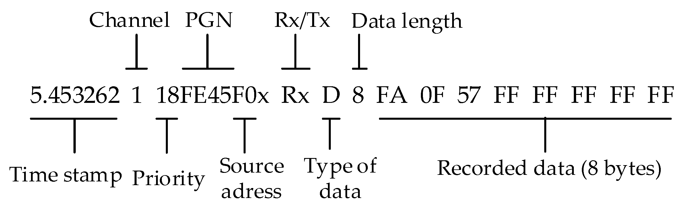
The GL2000 data logger was configured using its own configuration tool to filter the tractor’s ISOBUS communication data and record only messages with a specific parameter group number (PGN). An example of an ISOBUS message as it was retrieved from the data logger is presented in Figure 2. The ISOBUS messages that were used for the present research work are listed in

Table 1. Messages used for the area-related analysis.

Message	PGN/ID	Content
RHS	FE45	Rear Hitch Status
WBSD	FE48	Wheel Based Speed, Direction and Distance
Msg2	1FFFFFD1	D-GNSS Latitude and Longitude

, with their PGN indicated as a hexadecimal value according to part 7 of the ISO 11783 standard [19]. They were recorded with a frequency of 10 Hz. One of the recorded D-GNSS messages was also relevant for the area-related analysis and it is listed in Table 1. The D-GNSS messages did not originate from the CAN-Bus, but the data logger embedded them into the log files with a frequency of 1 Hz. The structure of these messages was basically the same as shown in Figure 2. However, their ID was defined specifically by the logger’s manufacturer. The acquired D-GNSS position data are presented in Figure 3. and are indicated as green dots. They can be assigned to the field “Schlag 5” of the examined farm, with a size of 2.90 ha as this was indicated in the field catalogue.

2.3. Data Analysis Flow

For data analysis, the MATLAB R2016b (The MathWorks Inc., Natick, Massachusetts, USA) programming environment was used. The main data analysis steps are presented with the main MATLAB functions in Figure 4. From the data editing to the modeling of the plow points, there was a continuous flow. The absolute values for the cultivated area and the area of the field boundary, as well as the overlapping, were directly derived from the modeled plow points. The calculation of indicators for the overlapping, except the plow points, required the identification of the cultivated area and the boundary value.

2.4. Data Editing

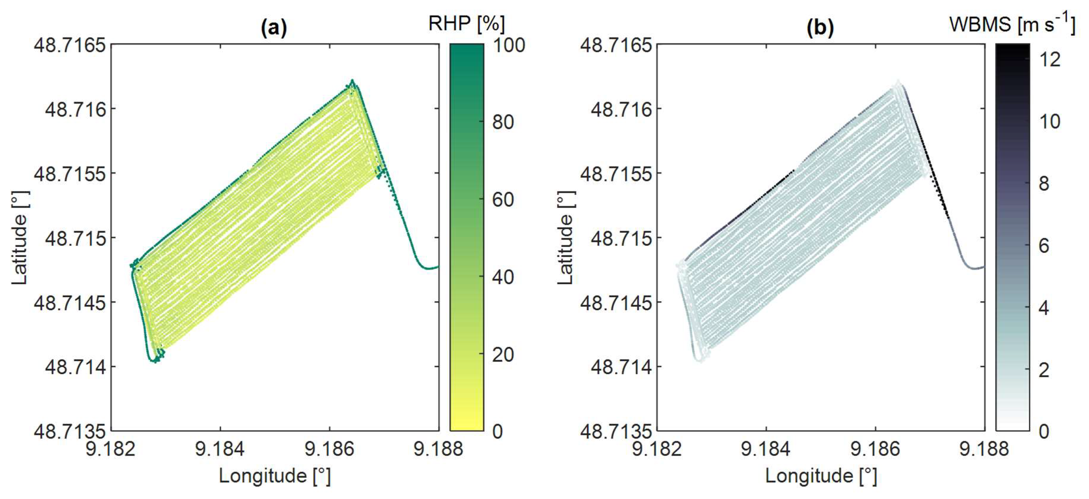
The first important information from the ISOBUS was the wheel-based machine speed (WBMS), which is the value of the speed of the machine as calculated from the measured wheel or tail shaft speed [19]. It is specified in meters per second and, similar to the corresponding timestamps, it was derived from the WBSD messages using the suspect parameter number (SPN). Expressed in hexadecimal values, the WBMS has the SPN “1862”. In the next step, the RHS messages from the ISOBUS were split into their time stamps and the rear hitch position (RHP), which has the SPN “1873”. The RHP is the measured position of the rear three-point-hitch, expressed as a percentage of full travel, whereby 0% indicates the full down position, and 100% the full up position [19]. Finally, the D-GNSS latitude and longitude according to the world geodetic system 84 (WGS 84), as well as their timestamps were deduced from Msg2 (see Table 1). The acquired data for the signals RHP and WBMS are presented in Figure 5a,b, respectively.

To enable a concurrent analysis at a specific point and to increase the resolution of the D-GNSS information, a linear interpolation of the WBMS, as well as the D-GNSS latitude and longitude, was performed using the MATLAB function “interp1”. The RHP time stamps were the query points for the interpolation, whereas the sample points were the time stamps of the WBMS and D-GNSS. As the positioning error of the used D-GNSS receiver, as well as the excitation of the tractor cabin, caused a jittering of the recorded track, a Savitzky–Golay filtering was applied using the MATLAB function “sgolayfilt”. The polynomial order of the filter was set to one because it best fit the chronologic sequence of the recorded track. A frame length with a value of 25 was considered to give a smoothing that represents the real track of the rover in a suitable way.

2.5. Filtering for Passes

A pass was supposed to contain all the in-work points from a lowering up to a lifting of the plow. The in-work points were defined as the timestamps with their corresponding RHP, WBMS and D-GNSS information, where the plow was assumed to be set in operation. The analysis started with the second value of each dataset, as every RHP value was compared to the preceding one. As soon as it fell below a threshold of 60%, the event was recognized as a lowering point. As an in-work condition for the subsequent points, the WBMS at a query point had to exceed a threshold of 0.134 m s⁻¹. As soon as the RHP exceeded again the threshold of 60%, a lifting event was detected. To facilitate geometric calculations, the D-GNSS information assigned to in-work points was transformed from latitude and longitude to northing and easting using the universal transverse Mercator (UTM) projection.

The above-mentioned in-work thresholds for the RHP and WBMS were determined manually after some trials on the data, without a deeper examination of the real tractor–implement combination or plowing process. Using the MATLAB function “histogram”, two histograms were created in the run-up to the filtering for in-work points. Figure 6a,b shows the histograms for the RHP and the WBMS, respectively. The bins indicate the number of elements for each parameter. The range of the RHP values was set from 0% to 90% to exclude the numerous 100% counts originating in a large part from road transport. To enable a focus on the in-work points, the range of the WBMS values was set from 0 to 4 m s⁻¹. The RHP histogram clearly indicates the distribution of the in-work positions. The upper edge is at about 50%. To confirm that all real in-work points were included, the threshold was set to 60%. As it can be observed in Figure 6b, the pattern for the WBMS was not so clear and thus not a useful indicator. The threshold was finally set after the effect of different values was visually analyzed on a plot of the in-work D-GNSS positions.

2.6. Distinction of Field Parts

To enable a distinct analysis of the lateral overlapping between the passes and the overlapping between the main part and the headlands, a distinction of the field parts had to be performed. As a preparatory step, the rough direction of every pass was expressed by a pass-vector created from the lowering to the lifting point. First visual assessments of the data resulted that the very first pass was also the first main part pass, which is usual for a plowing operation.

The distinction of the field parts was performed by calculating first the angle between the vector of the very first main part pass and every other pass of a field. To do so, the following formula was applied:

$$\mathit{\alpha }={\cos }^{-1}\left(\frac{\overrightarrow{\mathit{a}}\circ \overrightarrow{\mathit{b}}}{|\overrightarrow{\mathit{a}}|\cdot |\overrightarrow{\mathit{b}}|}\right)$$

(1)

where $\mathit{\alpha }$ is the angle between two vectors $\overrightarrow{\mathit{a}}$ and $\overrightarrow{\mathit{b}}$. When the value for the angle was within the range of 45–135°, the arbitrary pass was declared as a main part pass. Otherwise, it was declared as a headland pass. Figure 7 schematically illustrates the operating principle of the field part distinction algorithm. The long passes represent the main part, whereas the two headlands are represented by the short passes running perpendicular.

To distinguish the two headlands of every field, k-means clustering was performed on their D-GNSS data. The MATLAB function “kmeans” was using a k-means++ algorithm according to Arthur and Vassilvitskii [20]. The number of clusters was manually pre-set to a value of two according to the number of headlands.

2.7. Modeling of the Representative Plow Points

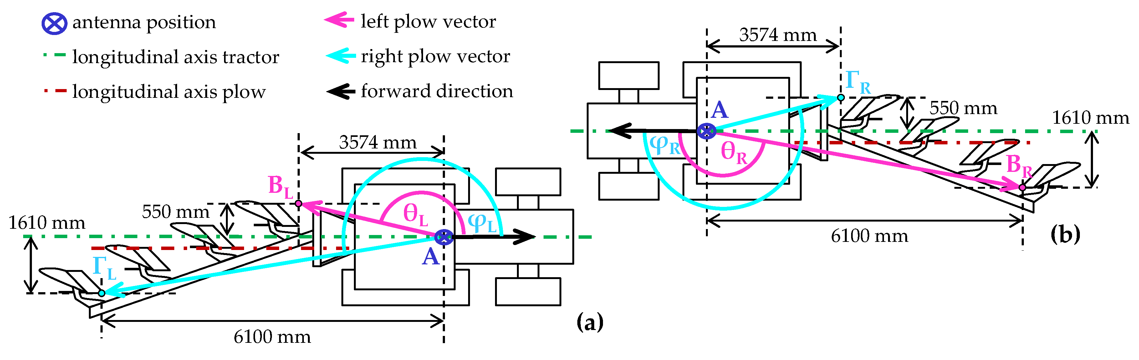
As a preparatory step, relevant sizes were taken from the real tractor–implement combination, whereby the working width was set to its maximum. In Figure 8, the modeling of the representative plow points is schematically illustrated and the relevant dimensions are indicated. Figure 8a shows the plow rotated on the left rotating position, while Figure 8b shows the plow rotated right. The figure is kept abstract because it is supposed to serve only as a schematic illustration. To enable a better overview, only the shares that are operating in each case are presented. A distinction of the two rotating positions is important because they represent two mirror-inverted arrangements of the working tools, which has an important effect on the reconstruction of the cultivated track.

For every rotating position separately, two points were defined that represented the lateral edges of the working width (points B and Γ). As can be seen in Figure 8a,b, the representative plow points are formed by first drawing a line parallel to the outer edge of the first and last share and crossing it with a perpendicular line, which is touching the front top of the shares. Then, this intersection point is projected vertically to the height of the antenna (Point A) to get the representative plow point. For the subsequent calculations, the left and right plow vectors pointing from the antenna to the representative points of the plow were created. Then, the φ angle (φ_L and φ_R for both rotating positions) and the θ angle (θ_L and θ_R for both rotating positions) were determined. They represent the angle between the forward direction and the left and right plow vectors. Furthermore, the length of the left and right plow vectors for both rotating positions (AB_L and AB_R, and AΓ_L and AΓ_R, respectively) was determined. The values for these dimensions, which indicate the position of the representative plow points relative to the antenna position, are presented in

Table 2. Relevant dimensions for the modeling of the representative plow points.

Rotated Left		Rotated Right		Unit
Parameter	Value	Parameter	Value
θL	171	θR	165	°
ABL	3616	ABR	6309	mm
φL	195	φR	189	°
AΓL	6309	AΓR	3616	mm

.

Several adjustment options of the plow have a substantial effect on its effective working width. As the logged data could not deliver exact information about the work state, assumptions were made concerning the main parameters. The working width was assumed to always be set to its maximum during the data acquisition. In fact, this was plausible, as the tractor had a relatively high power compared to the plow’s size. Concerning the rotation status, a simplified scheme was developed and applied to simulate this special characteristic. First, a distinction of passes having the same direction as the very first pass of a field part and passes running in the opposite direction was performed. For this, the angle between the vector of the very first and all other passes of a field part was determined using Equation (1). If the angle was between 0° and 45°, the pass was declared as running in the same direction as the very first pass. Then, the plow was assumed to be rotated right according to the definition in Figure 8. If it was between 135° and 180°, it was assumed to belong to a pass running in the opposite direction and, thus, rotated left.

2.8. Determination of the Cultivated Area

Figure 9 schematically illustrates the modeling of the cultivated area for three exemplary passes. To determine the driving direction, for every point of a pass, a vector was created, which originated in the D-GNSS position and pointed to the position of the chronologically subsequent position point. Thus, there was a vector indicating the direction at every point of a pass except for the lifting point, which was the very last point of a pass. For every pass, the left and right plow points marked the outer edges of the track that the plow had left during its operation. Using the previously outlined measures for the points representing the edges of the plow and setting them in relation to a static unit vector, which was parallel to the UTM easting and pointing eastwards, the absolute position of the representative points could be determined for every antenna position within a pass. To model the kinematics of the plow during work and thus smooth the track, a Savitzky–Golay filter was applied on the D-GNSS positions of the tracks using the MATLAB function “sgolayfilt”. In this case, a polynomial order of one and a frame length of 49 were applied. Very short passes with several in-work points below this frame length had to be removed in advance. All the points of a track could finally be connected to a polygon that was supposed to represent the cultivated area of a specific pass. The area of the main part and headland passes was calculated and added up to the total cultivated area of the field ($A_{total}$).

2.9. Determination of the Field Boundary

The automatic determination of the boundary was configured to give the D-GNSS coordinates of the outermost representative plow points encompassing all the cultivated tracks within the field. The maximum shrink factor of the corresponding MATLAB function “boundary” was applied to get the most compact boundary possible. A polygon was formed using the boundary points and its area ($A_{boundary}$) was calculated using the MATLAB function “polyarea”. To enable an examination of the boundary within a geographic information system (GIS), a keyhole markup language (KML) file was created, which contained all the WGS 84 coordinates of the boundary points. For this, the MATLAB function “kmlwritepoint” was used.

2.10. Determination of the Overlapping

Starting with the first main part pass, they were sequentially analyzed in terms of the lateral overlapping. The overlaps between the cultivated tracks of an arbitrary pass and the five chronologically subsequent passes were identified to ensure that no overlap was ignored. The overlap identification was done by determining for each comparison the intersection polygons and calculating their area. For this, the MATLAB functions “polybool (intersection)” and “polyarea” were used. The same process was performed on the headland passes. However, the overlaps between each cultivated track of a headland pass and all its chronologically subsequent ones were identified.

The overlaps between the main part passes and the headland passes were determined separately. Technically, the analysis procedure was the same as for the lateral overlaps. In this case, however, for every main part pass of a field, the overlaps with all the headland passes were identified. Naturally, it was possible that there was concurrently a lateral overlap and a headland overlap at locations, where main passes reach into the headland. They were respected separately in the calculations. 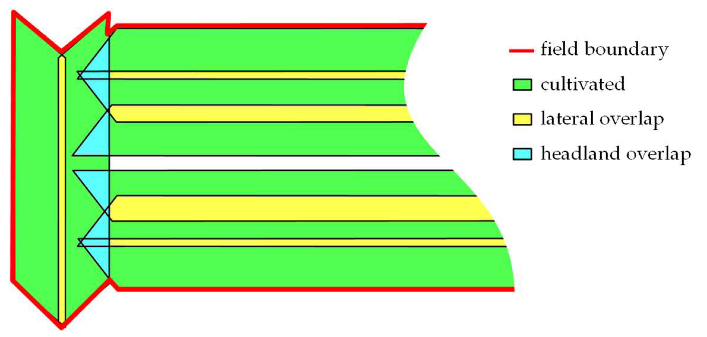Figure 10 illustrates the conception of the boundary and overlaps in an idealized way. The main part passes are running in an east–west direction and the headland passes are running in a north–south direction.

To enable a differentiated analysis of the overlapping within the field, different intermediate figures were determined. For the $A_{overlap,lat}$, the area of all lateral overlaps of the field was added up. The total headland overlapping for every field is expressed by $A_{overlap,head}$, which is the summed area of all overlapping polygons resulting from the intersections between the headlands and the main part. The first visual assessments of the modeled cultivated tracks uncovered noticeable lateral overlaps alternating with uncultivated lateral gaps due to the receiver error. Thus, the overlapping was corrected with the area of the gaps ($A_{gaps}$), which was calculated as follows:

$$A_{gaps}=A_{boundary}-(A_{total}-\left(A_{overlap,lat}+A_{overlap,head}\right))$$

(2)

A dedicated analysis of the lateral overlapping was enabled by calculating the $A_{overlap,lat,perc}$, which indicates the relation between the area of the corrected lateral overlapping and the total cultivated area within a field:

$$A_{overlap,lat,perc}=(A_{overlap,lat}-A_{gaps})/A_{total}·100\%$$

(3)

To enable a distinct assessment of the headland overlapping, the $A_{overlap,head,perc}$ was determined as an indicator for the relation between the summed area of headland overlaps and the total cultivated area of a field:

$$A_{overlap,head,perc}=A_{overlap,head}/A_{total}·100\%$$

(4)

$A_{overlap,perc}$ is considered the adequate indicator for the total overlapping within a field. It was calculated as follows:

$$A_{overlap,perc}=\left((A_{overlap,lat}-A_{gaps}\right)+A_{overlap,head})/A_{total}·100\%$$

(5)

Thus, it is the sum of $A_{overlap,lat,perc}$ and $A_{overlap,head,perc}$.

To compare the $A_{overlap,perc}$ with a more common indicator, which indicates the overlapping percentage within a field, the $A_{overlap,perc,ref}$ was calculated additionally:

$$A_{overlap,perc,ref}=\left(A_{total}-A_{boundary}\right)/A_{boundary}·100\%$$

(6)

The $A_{overlap,perc,ref}$ was inspired by how Demmel et al. [5] set the total cultivated area in relation to the area of the field boundary. This is a common way to express the overlapping by means of commercially available PF terminals.

3. Results and Discussion

3.1. Distinction of Passes

Fifty-eight passes could be detected by applying the algorithm for the distinction of passes. It matched with the number of lifting and lowering points, which is an important indication for the algorithm’s functionality. Figure 11a presents the D-GNSS position data of the lowering, lifting and in-work points with the corresponding RHP values, while Figure 11b highlights a zoomed area for a more detailed representation. Some single lowering and lifting points comparatively far away from the headlands can be observed in Figure 11a. This could indicate, e.g., corrections by the driver where he lifted the plow, moved back some distance and lowered it again to correct a driving error. Another explanation would be wedges at the field boundary where it is not necessary or rather possible to complete the whole pass.

In Figure 11b, the main part running in the southwest–northeast direction can be distinguished from the shorter headland running perpendicular. Furthermore, a varying distance between all passes is obvious. This was well expected by using a low-cost D-GNSS receiver. The work in [21] considers the pass-to-pass average error, which is also defined as the relative error, as the most important error for dynamic positioning. This relative error varies with the same receiver due to the testing date and time as well as vehicle speed and it highly depends on the used receiver.

As the RHP values were slightly below the in-work threshold of 60%, it was easier to visually distinguish the variations. It is interesting that the RHP had comparatively low values for passes at the edges of the main parts and headlands. This was the first indication for a specific driving scheme in these areas. These schemes can be varied and depend on the local conditions as well as the driver’s preferences. In the case of a reversible moldboard plow, this could indicate, e.g., a reduced working width by only setting the last few shares in operation or even a deviation from the usual plow rotation scheme.

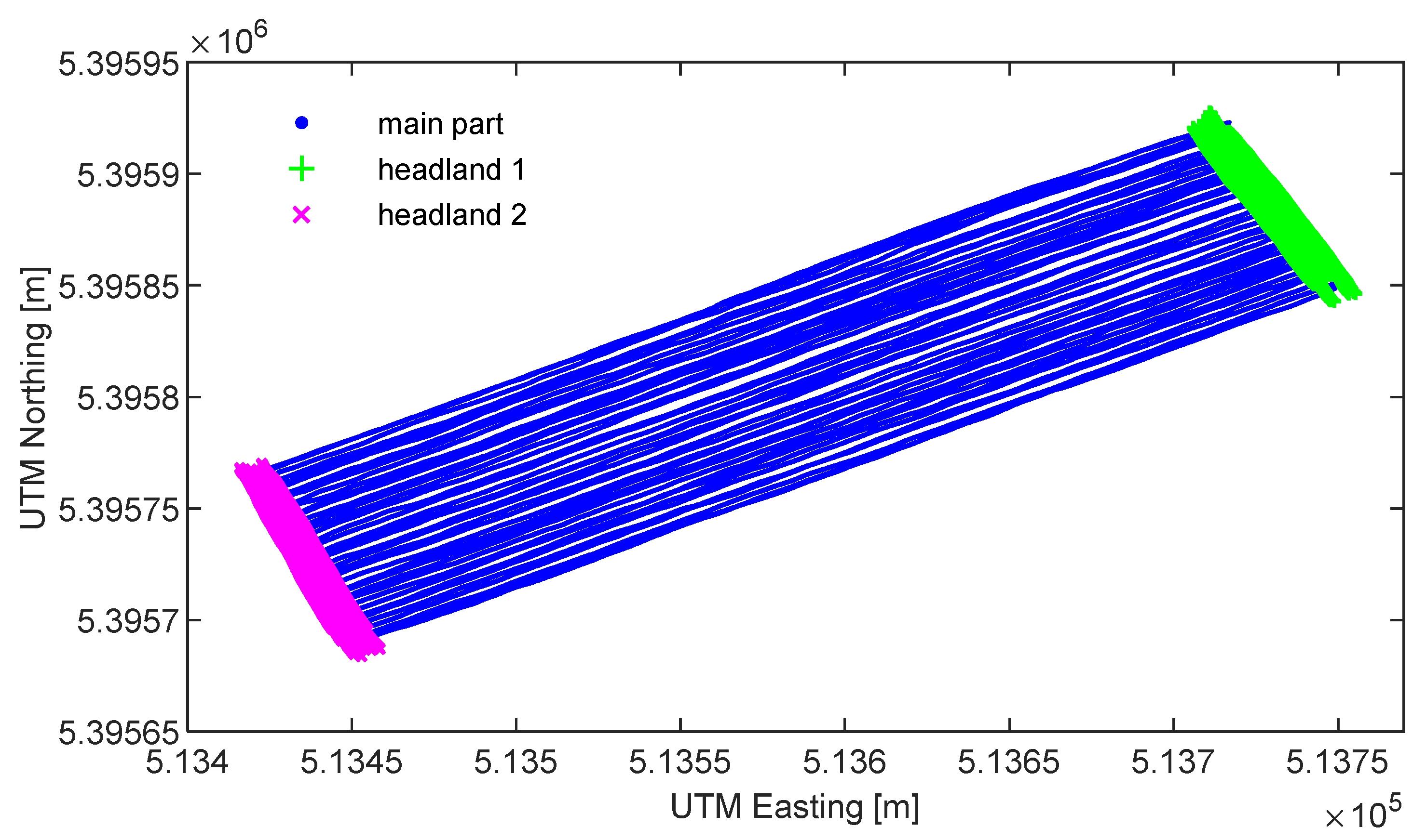
3.2. Distinction of Field Parts

In Figure 12, the main part as well as the two headlands can be distinguished for the examined field. After the extraction of passes with fewer than 49 in-work points, which was the Savitzky–Golay filtering frame length, 55 passes remained. Of these, 41 corresponded to the main part and seven to each of Headland 1 and Headland 2. It must be noted that the algorithm for the distinction contains simplifying assumptions and thus can only be applied to well-structured fields such as the examined ones. There is an enormous variety of fields with more complex geometries and constellations of main parts and headlands. The thresholds for the angle between the pass vectors could be adapted but the algorithm hardly contains any scope for further adaptions.

The distinction between the two headlands for every field using k-means clustering was a prerequisite for a differentiated analysis of the overlapping and it enabled making assumptions for the rotation scheme of the plow separately for every headland. Here again, simplifying assumptions were made. For more complex field geometries and fieldworks, it is possible to have some more areas that can be defined as headlands or to even have no headland at all. Even though the number of headlands could be adjusted for every field separately, the developed logic contains hardly any scope for further adaptions. Another aspect is the inability of the algorithm to clearly identify an individual headland. Due to the used k-means clustering, the determination, if a headland is the “Headland 1” or “Headland 2” of a specific field, has a random character.

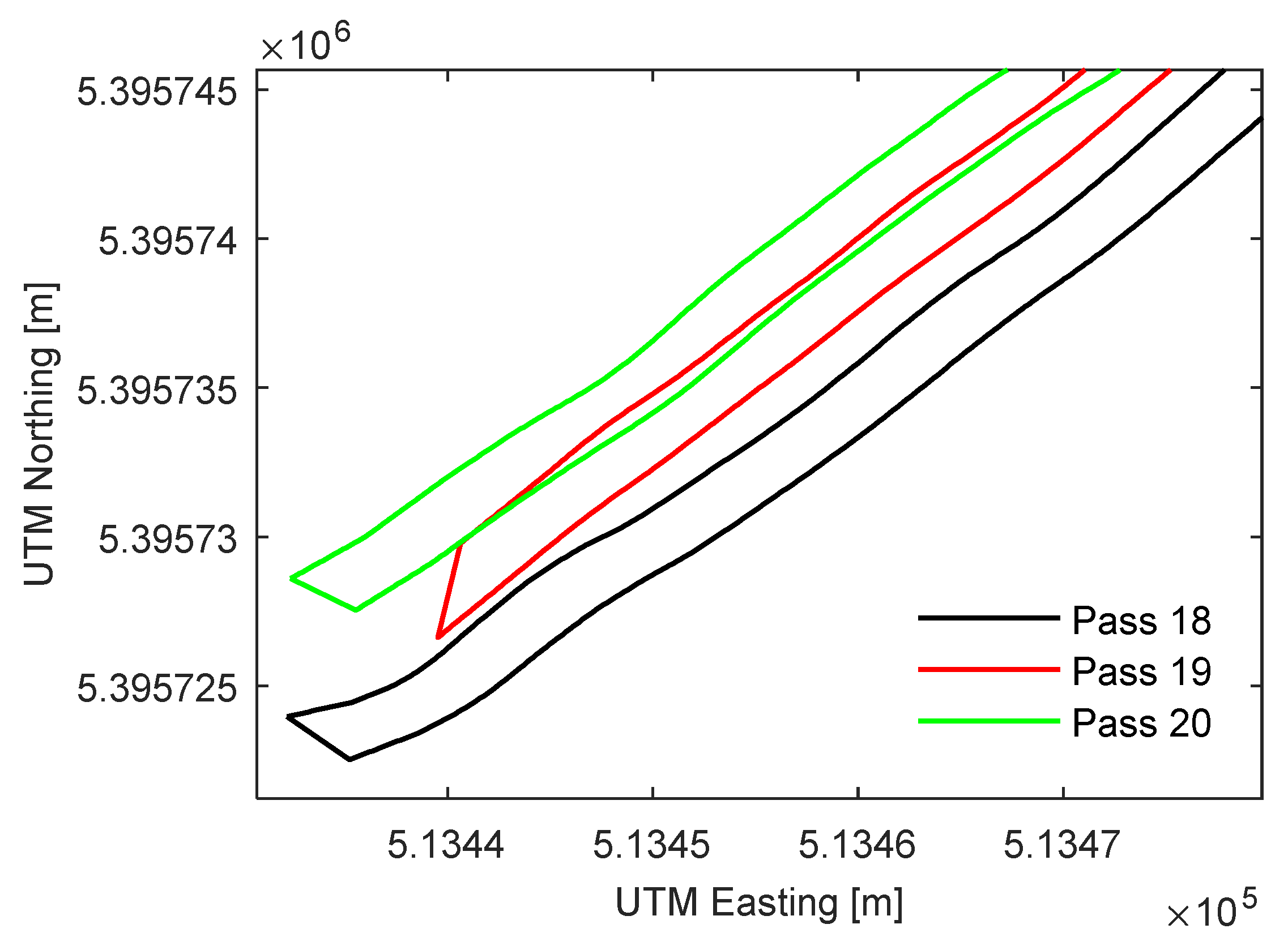
3.3. Cultivated Tracks

For every point of a pass, except for the last one, two points, which represent the lateral edges of the plow, were created depending on the current direction of movement. Under simplifying assumptions, a distinction was made between the two possible rotating directions of the plow. To get an idea of how a pattern of multiple cultivated tracks within the field looks, Figure 13a shows a zoomed area at the northeast corner of the field. The D-GNSS positions of the antenna are plotted together with lowering and lifting points indicating the passes. Furthermore, the representative plow points are illustrated. “Plow left” and “plow right” represent the left and the right edges, respectively, of the plow relative to the current driving direction (see definition of points B and Γ in Section 2.7). For a better representation, Figure 13b focuses on three exemplary passes (Passes 18–20) from the main part. They are representative of the regular operation scheme of the inner main part passes. The rotating position is not indicated separately, but can be derived from the arrangement of the left and right plow points at the beginning or the end of a pass.

Regarding the results discussed here, it could be argued that the filtering of the D-GNSS data was done arbitrarily to obtain a subjectively optimal smoothing. However, after several trials, it became clear that the effect of shifting the focus of the filtering to the interpolated raw D-GNSS data or to the cultivated tracks was negligible. Furthermore, the degree of filtering had in general only a minimal effect on the values of the area-related parameters, which are presented in the subsequent sections.

3.4. Cultivated Area

For the examined field, a total cultivated area $A_{total}$ of 3.13 ha was determined. Figure 14 presents a part of the cultivated area that corresponds to the same exemplary passes that are presented in Figure 13b. A lateral overlapping can be distinguished between Passes 19 and 20. Furthermore, a gap area is noticeable between Passes 18 and 19. This does not mean that this area was left uncultivated, but it originates from the D-GNSS position error and justifies the choice to subtract from the lateral overlapping area $A_{overlap,lat}$, the total gap area $A_{gaps}$ (see Equation (3)). Furthermore, a remaining jittering of the tracks became obvious. After some visual assessments, this was considered as some kind of noise that had to be accepted to not cause a strong idealization by over-filtering.

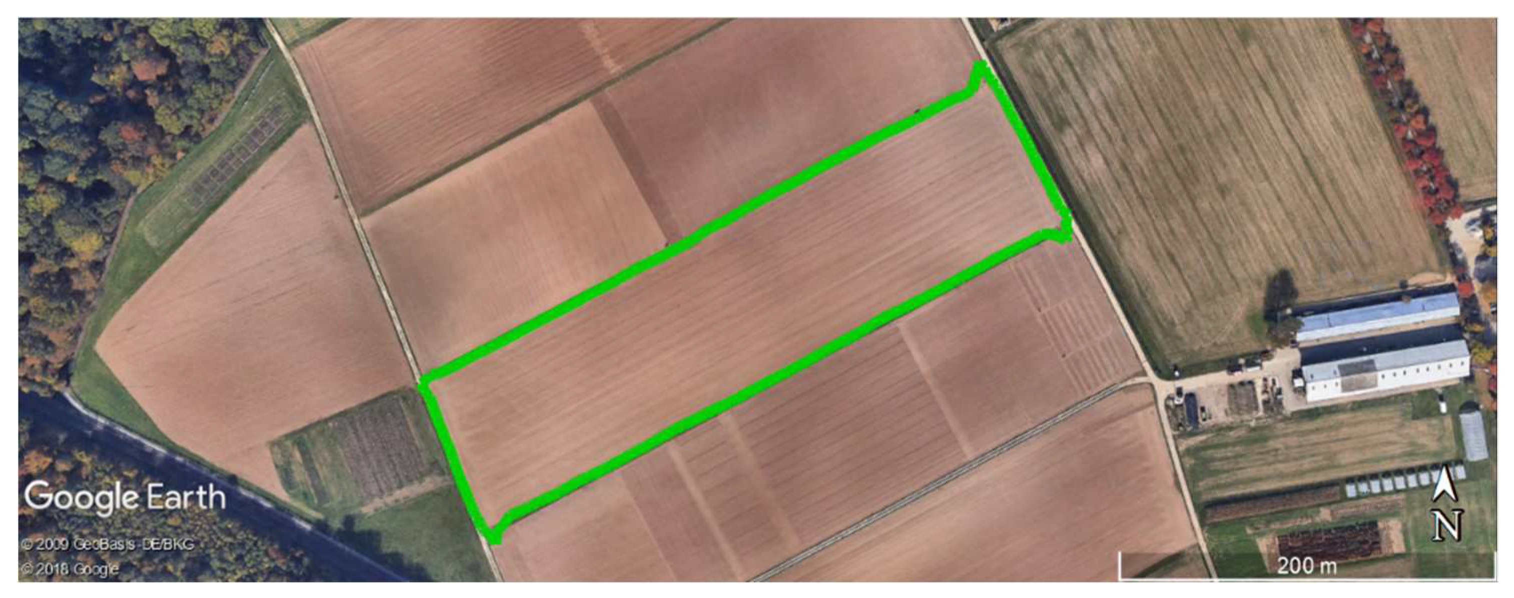
3.5. Field Boundary

The area of a boundary should represent the specific field size and location, as documented in the field catalogue (2.90 ha). It was calculated by the developed software with $A_{boundary}=$ 2.94 ha, which results in an overestimation of 1.4%. Figure 15 shows a satellite view of the boundary (indicated in green) for the examined field. It fits the actual field location. Several error sources influenced the determination of the boundary. The erroneous D-GNSS positioning had an effect, especially at the field edges. A further influence negatively affecting the determination of the boundary was that the applied shrinking of the MATLAB function “boundary” could not deliver the closest fit possible. Furthermore, what is assumed to cause error is the deviation from the plow rotation scheme or a variation in working width, especially at the beginning and the end of a field part. Another possible error source is the rolling of the tractor while driving on a slope along the field edges. All these errors could not be monitored and corrected. Considering these errors, the deviation of 1.4% from the actual field size is a strong indication of the efficiency of the developed algorithm.

3.6. Overlapping

Figure 16a shows the field boundary, the cultivated tracks, and the lateral and headland overlaps. For a more detailed representation, Figure 16b presents a zoomed area at the lower northeast corner of the field. It must be stated that the color highlighting of the headland overlaps is virtually dominant.

In Figure 16b, the fact that the used function for the determination of the boundary could not deliver the closest fit possible is illustrated. Beyond an overestimation of the field size, this also caused an overestimation of the gaps’ area $A_{gaps}$ and, thus, an underestimation of the summed area of lateral overlaps $A_{overlap,lat}$. Furthermore, there are noticeable distortions at the tops of several headland tracks, which was a further source of error concerning the boundary. They could be traced back to the error behavior of the used receiver. The discrepancy between different errors depending on the rover’s movement has been examined previously (e.g., [22,23]). A further possible source of error was the overall additional excitation of the tractor cabin during headland overlapping.

In Figure 16b, passes can be distinguished where there is an excessive lateral overlap alternating with gaps in the magnitude of the plow’s working width. This was mainly due to the erroneous D-GNSS positioning, as discussed in previous sections. The pass-to-pass error of low-cost receivers has been considered previously (e.g., [21]). Furthermore, it can be recognized that two of the first main part passes in the south are almost entirely overlapping, whereas there seems to be no corresponding gap. For the rest of the field, this was also a common pattern for some of the first and last few passes of the main part or a headland, indicating again a specific driving scheme at these sites. This pattern fits the observations discussed in Section 3.1 and led to an overestimation of $A_{overlap,lat}$.

A typical problem with moldboard plows are the undesirable triangular shapes of unplowed segments at the headlands [15]. Headland overlapping is generally an important indicator of the performance of the driver, having a remarkable effect on the field efficiency and causing additional cost. The alignment of the beginning and the end of the main part tracks, which can be observed at the top of the polygons, is highly variable in Figure 16b. Possible reasons for this observation were a varying track-error of the D-GNSS positioning and improper timing by the driver. In general, the headland overlaps seem to be quite long. An obvious reason for that was the remaining error for the setting of the in-work threshold of the RHP, as described in Section 2.5. However, a minimization of the threshold would have had little effect on the length of the pass and probably would have led to an exclusion of points that were only just tilled. The main results in terms of the overlapping indicators are listed in

Table 3. Overlapping indicators.

Indicator	Value [%]
$A_{overlap,lat,perc}$	2.05
$A_{overlap,head,perc}$	3.96
$A_{overlap,perc}$	6.01
$A_{overlap,perc,ref}$	6.39

.

$A_{overlap,lat,perc}$ contains the same information as the efficiency of width use, which is documented in [24]. When transferring the values given in this reference to the $A_{overlap,lat,perc}$, it should not exceed a value of 5%. Considering the numerous previously mentioned error sources and simplifying assumptions, the value of 2.05% seemed usable for a first estimation.

$A_{overlap,head,perc}$ refers only to the overlapping between the main part and the headland passes and was set in relation to the total cultivated area. When comparing the value of 3.96% to the $A_{overlap,lat,perc}$, it became obvious that the headland overlapping had an even bigger influence on the total overlapping within the field than the lateral overlapping between neighboring passes.

$A_{overlap,perc}$ is the sum of $A_{overlap,lat,perc}$ and $A_{overlap,head,perc}$ and indicates the total overlapping within the field boundary. To compare it with a more common way to express the overlapping within a field, the values for $A_{overlap,perc,ref}$ are also indicated in the table. Similar to Demmel et al. [5], the total cultivated area of a field was set in relation to the area of the field boundary. The value was slightly higher than $A_{overlap,perc}$. This was natural because the area of the boundary as a reference was lower than the total cultivated area. $A_{overlap,perc,ref}$ was almost unaffected by the relative error of the positioning; only a small error could be expected for the actual boundary size. This implies that the imperfect information about the actual work state of the plow had the most negative effect on the results concerning the overlapping indicators.

4. Conclusions

A methodology was developed that enabled a distinction of work sequences from non-work sequences using a few parameters retrieved from a tractor’s ISOBUS. A field part distinction was applied as a prerequisite for a differentiated area-related analysis. A modeling of the cultivated tracks, based on the way the plow covered the area step-by-step, was implemented. Based on that, the cultivated area was quantified and the field boundary was detected in terms of location and size. Finally, different indicators were developed and calculated for the overlapping. An assessment with a more common indicator proved the plausibility of the results. Incomplete information about the work state of the implement, erroneous D-GNSS positioning and a limited shrinking of the boundary were identified as the main sources of error.

Automated, detailed detection of the cultivated area and the field boundary can be very valuable, e.g., for documenting and invoicing of agricultural tasks within networked software infrastructures. A differentiated analysis of overlapping can serve as an indicator of efficiency. In future work, the presented parameters for the overlapping analysis should be validated on fields of different sizes and geometries.

If there were more detailed information about the actual work state of the plow, more reliable results could be expected. The new generation of ISOBUS-enabled plows is very promising in delivering this information. Furthermore, the use of more accurate positioning and data acquisition instrumentation is recommended when a higher level of accuracy is required. One possibility would be using real time kinematic GNSS and robotic total stations [25]. Another option would be fusing information from GNSS receivers and inertial sensors, a technology which is already implemented in commercial automated steering systems. Considering these possible improvements, the slight overestimation of 1.4% in terms of the boundary’s size is promising for the potential use of more sophisticated applications, e.g., automated steering. With a few adaptions, the used methodology for an area-related analysis could be transferred to a wide range of mounted soil tillage implements and plant production processes.