Article

Spatial Correlations between Nitrogen Budgets and Surface Water and Groundwater Quality in Watersheds with Varied Land Covers

Water Environment Research Department, National Institute of Environmental Research, Hwangyong-ro 42, Seogu, Incheon 22689, Republic of Korea
*
Author to whom correspondence should be addressed.
Agriculture 2024, 14(3), 429; https://doi.org/10.3390/agriculture14030429
Submission received: 7 February 2024 / Revised: 4 March 2024 / Accepted: 4 March 2024 / Published: 6 March 2024
(This article belongs to the Special Issue Integrated Management and Efficient Use of Nutrients in Crop Systems)

Abstract

:
Anthropogenic nitrogen (N) inputs can have detrimental environmental effects, necessitating a comprehensive understanding of the nitrogen budget (NB) and its spatial correlation with the water quality. This study, utilizing a 2016 dataset, scrutinized 850 subwatersheds with diverse land covers across the Republic of Korea (ROK). Employing Geographically Weighted Regression (GWR), it examined the spatial correlations between the NBs and the quality of the groundwater and river water at the watershed scale. Robust correlations (R2 = 0.87) were observed between the groundwater quality and NBs, surpassing those of the surface water (R2 = 0.48). Sensitivity analyses highlighted the importance of high-resolution spatial data in capturing nuances within complex land covers. The integration of such data led to increases in the spatial correlations between the groundwater and river water quality of approximately 0.6–0.9 and 0.3–0.5, respectively. Notably, when the agricultural land cover exceeded 10%, significant enhancements in the spatial correlations were observed, emphasizing the pivotal role of agriculture in nutrient and water quality. At a 10% cropland ratio, the spatial correlations between the watershed-scale NBs and river/groundwater quality increased by approximately 76% and 501%, respectively. This study provides novel insights into the spatial relationships among NBs, water quality, and land use, highlighting the significance of high-resolution data and the impact of agricultural practices on watershed management. These findings contribute valuable information for developing strategies to mitigate nitrogen pollution.

Graphical Abstract

1. Introduction

In aquatic ecosystems, nutrients, specifically nitrogen (N) and phosphorus (P), play a pivotal role in maintaining the biodiversity and equilibrium [1]. N is one of the primary components of all constituents of aquatic ecosystems and is essential for biological activities, such as the promotion of productivity and the utilization of energy sources [2]. However, the excessive supply of N due to anthropogenic activities not only adversely affects aquatic ecosystems, including through the proliferation of harmful algae, habitat destruction, and the contamination of drinking water, but also poses significant threats to human health [2]. The supply of N in water bodies has shown a persistent increasing trend [3], with a particularly rising proportion being discharged from agricultural areas; hence, it is the primary contributor to the impact on aquatic ecosystems [4,5]. Consequently, the management of spatially distributed N sources in agricultural watersheds has become imperative to ameliorate the water quality [6,7,8].
There are various anthropogenic N pollution sources in agricultural areas. An increase in N occurs when the quantity of mineral fertilizers applied for crop production exceeds the amount required by the crops [9,10]. Moreover, the escalation in the number of livestock due to intensive farming increases the supply of N [11]. While animal waste is recycled in forms such as solid or liquid composted manure [12,13], its use in conjunction with fertilizers contributes to environmental contamination through nonpoint-source pollution [14,15].
The nutrient budget is an indicator used to evaluate the nutritional status in agricultural environments [16]. The Organisation for Economic Co-operation and Development (OECD) utilizes the nutrient budget as a benchmark for international comparative analyses of the environmental pollution nutrient statuses in agricultural areas [17]. The nutrient budget is defined as the differences between the nutrient inputs (e.g., mineral fertilizers, livestock excreta, atmospheric deposition, and N fixation by legumes) and outputs (cultivated crops) of N and P over a specified temporal and spatial scale [18]. The nutrient surplus determined in the nutrient budget conceptually encompasses nutrients transported to the environment, such as via leaching or runoff. Specifically, for the nitrogen budget (NB), atmospheric losses (e.g., volatilization) are also considered in the surplus [19].
The nutrient budget can also be used to assess the status of residual nutrients [20], enabling a quantitative evaluation of the impact on the surrounding environment from potential pollution sources [21,22,23]. Therefore, the nutrient budget can be utilized not only as an indicator for nutrient management but also to effectively manage watersheds, such as by assessing the impact on the water quality in various environmental media (e.g., rivers and groundwater) [17].
Regarding the NB, research has been conducted to assess N management [18,24,25], focusing on the N status within the watershed and analyzing the contribution of N sources. However, there remains a lack of studies evaluating the potential impacts of the indicators calculated through the NB on the water quality. Especially when considering the characteristics of various spatial distributions of N sources within watersheds, it is necessary to evaluate the spatial correlation between the NB and water quality [26,27,28,29].
In watersheds with complex land cover characteristics, a spatially diverse distribution of various N sources exists, with some being densely concentrated while others are scattered, exhibiting distinct characteristics [30,31]. As a result, the correlation between the NB and water quality could also manifest spatial variations across different watersheds [26,32]. Nonetheless, studies that scrutinize the spatial correlation between the NB distribution and quality of the surface water or groundwater across various watersheds characterized by diverse land covers are limited.
The Geographically Weighted Regression (GWR) method of analyzing spatial correlation has been utilized as a valuable tool for evaluating spatial causality [33,34]. Numerous studies investigating spatial water quality characteristics using GWR have focused on analyzing the spatial correlation between the land cover characteristics, or the spatial distribution characteristics of pollution sources, and the water quality [35,36,37]. Therefore, GWR is a reliable tool for evaluating the spatial causality between NBs and the quality of surface water or groundwater [38,39,40]. To the best of our knowledge, this study is the first to evaluate the spatial correlation between the NB and water quality.
In this study, the feasibility and applicability of using NBs to assess the water quality in mixed-land-cover watersheds were examined. The main aims of this study were (1) to analyze the spatial correlation between the subwatershed-level NBs and surface water (rivers) and groundwater quality using GWR in subwatersheds with complex land covers; (2) to compare the spatial correlation between the NBs and water quality based on the differences in the spatial resolution of the water quality data; and (3) to examine the variations in the correlations between the NBs and water quality in rivers and groundwater based on land use characteristics.

2. Materials and Methods

2.1. Study Site

This study was conducted across the Republic of Korea (ROK), between latitudes 33° N and 43° N and longitudes 124° E and 132° E. The total land area of the ROK is approximately 109, 411.8 km2. The ROK persistently ranks at the top for N surpluses (http://data.oecd.org/agrland/nutrient-balance.htm, accessed on 30 November 2023). Given the diverse land cover characteristics across its watersheds [41], anthropogenic N is primarily discharged through a variety of N sources distributed across different land covers, influenced by hydrological factors [27,42].
The four major basins in the ROK are those of the Han, Geum, Yeongsan, and Nakdong rivers (Figure 1a); of them, the Han River has the largest area (38%), followed by the Geum (16%), Nakdong (29%), and Yeongsan (16%) rivers. Watersheds and subwatersheds are located within the 4 major basins, namely, 117 watersheds (Han River: 30; Geum River: 21; Nakdong River: 33; and Yeongsan River: 33) and 850 subwatersheds (Han River: 292; Geum River: 137; Nakdong River: 271; and Yeongsan River: 150). This study analyzed the spatial correlations between the NBs and the quality of the surface water (rivers) and groundwater at the subwatershed level (n = 850). The average size of the subwatersheds is approximately 129.0 km2, with a size range of 7.5–700.4 km2 (i.e., the size of the largest subwatershed is 100 times that of the smallest one). Derived from the 2017 land cover dataset, the analysis reveals that forested areas, agricultural land, and urban areas constitute approximately 60, 20, and 10% of the total land coverage, respectively (Figure 1c). The ROK is characterized by a monsoon climate, with the most annual precipitation (approximately 56% [710.9 mm] based on the average value for 1991–2020) concentrated in the summer months from July to September.
The elevation distribution range is 0–1944.6 meters above sea level, showing a decreasing trend from the eastern coast to the central and western regions (Figure 1d).

2.2. Geographically Weighted Regression

The GWR spatial regression technique accounts for spatial non-stationarity, implying that the relationships between variables can vary across spaces [39]. In GWR, the regression coefficients are estimated for each location within the study area, enabling spatially varying relationship identification and providing insights into regional spatial patterns [43]. In GWR spatial relationships, it is assumed that spatial autocorrelation determines the degree of similarity between the observations based on spatial proximity. A high level of spatial autocorrelation indicates that neighboring observations are more similar to each other than to those farther apart [44]. Spatial autocorrelation measures the extent to which nearby observations have similar values for a particular variable [44]. The GWR model is expressed as follows:
yi = β0(xi) + β1(xi) xi1 + … + βp(xi) xip + εi
where yi is the dependent variable for location i; xij is the jth independent variable for location i; βj(xi) is the coefficient for the jth independent variable at location i; and εi is the error term at location i. In GWR, similar to all regression analysis methods, model fit is important; a good fit indicates that the model adequately explains the spatial relationship between the variables [45]. In the current study, the R2 was used for the model evaluation, and the Spatial Analyst tool in ArcGIS version 10.4.1 (Esri, Redlands, CA, USA) was used to conduct the GWR analysis.

2.3. Nitrogen Budget

The modified NB equation utilized in this study was tailored to account for the characteristics of domestic livestock excreta treatment [16], resulting in the subdivision of the livestock excreta production section into three categories (Figure 2). Specifically, the excreta generation was targeted for the beef and dairy cattle, swine, and poultry species. The NB equation considers seven input components and two output components (Figure 2).
The N input included mineral fertilizers, livestock excreta, organic fertilizers, and materials for sowing/planting, with additional calculations for the biological N fixation and atmospheric N deposition. Livestock excreta was further classified into solid and liquid compost and wastewater treatment. Outputs were calculated based on the N quantities from crop production, including the crop yield, forage crop production, and plant residues. The comprehensive equations for the seven input and two output components, as well as the atmospheric and hydrospheric segments within the surplus, are presented in the Supplementary Materials (Table S1). Various coefficients for the NB calculations, including the livestock excreta volume per livestock unit, N content of fertilizers, and crop characteristics, were obtained from the literature. The parameters employed for each component are listed in the Supplementary Materials (Table S2).
The NB analysis utilized data from a 2016 survey and relevant information sourced from various institutions (Table S3). Statistical data from the Korea Statistical Office were used as inputs for mineral fertilizers (https://kosis.kr, accessed on 1 November 2022). Information on the livestock populations and treatment status by livestock species was obtained from the National Institute of Environmental Research (http://werms.nier.go.kr, accessed on 1 November 2022), and organic fertilizer data were obtained with the cooperation of the National Agricultural Cooperative Federation (http://www.nonghyup.com/eng/main/main.aspx, accessed on 1 November 2022).
Information regarding the N fixation, sowing/planting, forage crop production, and cultivation areas was obtained from the Agricultural Management Information System, which provides data from the Agricultural Management Organization (http://agrix.go.kr, accessed on 1 November 2022). The acquisition of diverse input data essential for NB calculations is facilitated through locally oriented administrative agencies. The spatial distribution of these annual data aligns with the administrative divisions. Consequently, despite variations in data sources for individual components, the temporal and spatial coverage collected remains uniform.
To compute NBs at the watershed level, it is imperative to ensure uniform spatial extents for each input and output category, grounded in the watershed boundaries. In this study, we addressed the spatial limitations intrinsic to input data organized at the administrative level by applying overlapping administrative area proportions within the watershed, which enabled us to re-evaluate the NBs within the subwatershed based on a revised spatial framework. Subwatershed-scale NBs were estimated by applying local administrative-scale NBs to the proportion of cropland area within the subwatershed.

2.4. Data Sources

2.4.1. Groundwater Quality

In the ROK, groundwater is monitored by various public agencies, such as the Ministry of Environment (MOE), Ministry of Land, Infrastructure and Transport, and Ministry of Agriculture, Food and Rural Affairs. These agencies conduct surveys for various purposes, including water quality monitoring and quantity management (Figure 1b). The groundwater quality is assessed 4 times annually at approximately 1200 monitoring sites. This study used the nitrate–nitrogen (NO3-N) concentration data from all monitoring points in 2016.
The annual average of the periodically observed data at each point was considered to enable comparisons with the annual NBs. The average NO3-N concentration in 2016 was approximately 3.3 mg/L, with a distribution range of 0–24.9 mg/L and a standard deviation of approximately 0.4 mg/L. Although the NO3-N concentrations across all sampled locations were diverse, seasonal variations in the NO3-N concentrations remained relatively small.

2.4.2. Surface Water Quality

The ROK MOE monitors the surface water quality monthly–quarterly at approximately 957 locations (Figure 1a). In this study, the analysis incorporated the annual average TN concentrations recorded at each river monitoring station in 2016 for the GWR analysis. A distribution range of 0–14.7 mg/L was observed for the TN concentrations in 2016, with an annual average concentration of approximately 3.1 mg/L.

2.5. Sensitivity Analysis of Data Resolution

Spatial correlation can yield varying outcomes due to differences in the data resolution [46]. In this study, the following methods were implemented to analyze the sensitivity of the correlation results based on the spatial resolution of the data distributed within the watershed: First, data with two different resolutions were constructed by averaging the observed values at each point distributed within the watershed with all the surveyed point data distributed within the watershed. Next, the spatial correlation between the data with two different resolutions and the NB results calculated on a watershed basis was derived, and the two results were compared. A comparative analysis of these two datasets examined the sensitivity to the spatial resolution.

3. Results and Discussion

3.1. Nitrogen Budget

The NBs were assessed for 850 subwatersheds in 2016. Delving into the specifics of the N inputs and outputs per component, the dominant contributor among the inputs was solid composted livestock manure (N 2-2), accounting for approximately 35% (Figure 3a). This prominence is attributed to the increase in livestock populations and the corresponding rise in the recycling rate of livestock excreta [47,48]. Other organic fertilizers (N 4) and mineral fertilizers (N 1) constituted approximately 28% and 25% of the N inputs, respectively. The relative significance of N 1 and N 4 can be attributed to the expansion of agricultural areas with lower soil fertility, necessitating increased fertilizer usage for crop productivity and crop production [49,50]. Notably, the N outputs were predominantly associated with crop production (N 9).
The NBs exhibited a range of approximately 11.4–490.5 kg/ha, with an average of approximately 210.5 kg/ha. Further analysis revealed that a significant portion (approximately 82%) of the NBs dropped within the range of 140–280 kg/ha across the subwatersheds (Figure 3b).

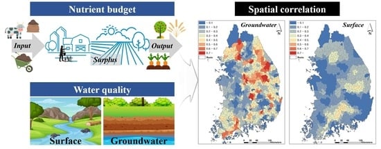
3.2. Spatial Correlation between NB and Groundwater and Surface Water Quality

GWR was used to analyze the spatial correlation between the NB and the quality of the surface water (rivers) and groundwater. Spatial correlation refers to the degree to which neighboring regions influence each other, indicating that data from adjacent locations are likely to exhibit similar patterns based on the local sources of pollution or land cover characteristics [40].
The distribution range of the spatial correlations (R2) between the nitrate concentrations of the groundwater- and subwatershed-scale NBs was 0.0–0.87 (Figure 4a).
The distribution characteristics of the spatial correlations at the subwatershed level indicated that approximately 52% of the subwatersheds showed correlations below 0.3, whereas those of approximately 15% were ≥0.5. The R2 values between the TN concentrations and subwatershed-scale NBs ranged from 0.0 to 0.48 for rivers (Figure 4b), with >90% of the R2 values being <0.1.
Spatial correlation comparisons between the NBs and water quality showed that the spatial correlations of the groundwater were higher than those of the surface water. Groundwater is influenced directly by land use and practices [51] and is replenished by water infiltrating the soil surface, and residual nutrients could affect the groundwater quality for an extended period [52,53]. Owing to its slow flow rate and longer residence duration in soil, groundwater is sensitive to changes in the water quality due to the input of residual soil nutrients [54,55]. Using GWR analysis, Koh et al. [33] found an association between the spatial distribution of the groundwater quality and land use and agricultural management practices.
In comparison, various factors influence the surface water quality, including diffuse pollution caused by rainfall and point-source pollution originating from sewage and wastewater treatment facilities. Nonpoint pollution sources are generally transported with rainfall [56] via agricultural activities; therefore, the surface water quality is significantly affected by the meteorological conditions. Following runoff, the surface water quality exhibits pronounced event-driven characteristics, with transient effects [57]. The pollutants in river water are highly mobile compared with those in groundwater, attributable to the faster flow velocity of rivers compared with that of groundwater [58]. Consequently, the direct and indirect influences on the spatial correlation between the annual NBs and surface water quality can be reduced [59,60].

3.3. Sensitivity Analysis of Data Resolution in Spatial Correlation

The spatial correlation sensitivity of the data resolution obtained using the GWR in the subwatersheds was analyzed for the river and groundwater quality. For this analysis, spatial correlations between the subwatershed-scale NBs and all monitoring data within the subwatershed were compared with those between the NBs and the spatially averaged data at the subwatershed scale.
The spatial correlation distribution between the NO3-N concentrations of the groundwater averaged at the subwatershed level and the NBs ranged from 0.0 to 0.60, indicating relatively lower correlations, compared with that between the NO3-N concentrations at individual groundwater-monitoring sites and the NBs (Figure 5a). Analysis of the spatial correlation distribution revealed that approximately 74% of the subwatersheds showed low spatial correlations of ≤0.1. In contrast, based on the individual monitoring sites, approximately 16% of the entire study area showed spatial correlations of ≤0.1. This suggests that employing data averaged at the subwatershed level to assess spatial correlations results in lower values compared with using all the data from individual monitoring sites.
The variations in correlation strength could potentially be attributed to the higher density of data points at the individual monitoring sites. While the averaged density of monitoring points per unit area (km2) was approximately 0.009 points/km2 and ranged from 0.001 to 0.048 points/km2, that of the spatially averaged data at the subwatershed scale was approximately 0.006 points/km2, spanning from 0.0003 to 0.048 points/km2. Therefore, using individual monitoring sites with higher data point densities produced a more robust spatial correlation with the NBs compared with that of the subwatershed-scale averaged data.
Spatial correlation analysis between the subwatershed-averaged TN concentrations in the river water and the NBs yielded a maximum correlation of 0.33 (Figure 5b), which was lower than the spatial correlation between the NBs and TN concentrations at the individual monitoring sites. Furthermore, when data from individual monitoring sites were used, approximately 35% of the subwatersheds showed spatial correlations of ≤0.1, whereas when subwatershed-averaged surface water quality data were used, >90% of the subwatersheds showed low spatial correlations (<0.1). This finding was similar to that for the groundwater, which indicates that employing subwatershed-averaged data results in a lower spatial correlation compared with that based on point-level data. The average density, considering every surface water observation point, was approximately 0.01 points/km2, ranging from 0.002 to 0.134 points/km2. In comparison, the density using spatially averaged data at the subwatershed scale decreased to approximately 0.007 points/km2, ranging from 0.001 to 0.134 points/km2.
These density variations further supported the observation that individual monitoring site data with higher data point densities exhibited stronger spatial correlations with the NBs than subwatershed-scale averaged data. A comparison of the data densities of the subwatersheds revealed a significant increase in high correlations when individual rather than subwatershed-averaged data were used. This observation suggests that subwatershed-averaged data have limitations in terms of the spatial distribution and variability within the subwatershed [61,62]. In subwatersheds with complex land cover characteristics, substantial variations occurred in data observed at individual groundwater sampling sites [63,64]. For instance, the maximum concentration of NO3-N measured at the groundwater-monitoring points was 24.9 mg/L in 2016, whereas the subwatershed-averaged NO3-N concentration was 14.7 mg/L.
Similarly, the average concentrations of TN in the river water based on individual point measurements and subwatershed-averaged data were 3.1 mg/L and 1.6 mg/L, respectively. This disparity underscores the importance of data resolution in capturing the spatial variations in TN concentrations.
The resolution of data plays an important role in delineating the spatial correlation between the water quality and NBs. Data with a high degree of granularity encapsulate a wide range of land cover types and multifarious N sources, providing insights into the N cycling processes. Conversely, data with coarser granularity, compiled at the subwatershed level, might not capture the microscale variability, which could potentially impede the precise detection of the N concentrations. In subwatersheds with a spectrum of land cover attributes, it is imperative to underscore the spatial distribution of and variability in the water quality [65].

3.4. Agricultural Area Sensitivity Analysis in Spatial Correlation

Recognizing the sensitivity of agricultural land use within the spatial correlation between the NBs and water quality in subwatersheds [61,62], the agricultural area distribution within the study area’s subwatersheds was examined. A histogram was used to determine the proportion of agricultural area in each subwatershed across the ROK (Figure 6), which showed that the 10% cropland category had the highest proportion of subwatersheds with agricultural areas. Moreover, more than 75% of all the subwatersheds exhibited agricultural areas exceeding 20%, which indicates that when the cropland area exceeds 20%, it accounts for less than 25% of the total subwatershed area across the ROK.
Notably, subwatersheds with croplands exceeding 20% displayed concentrated land cover characteristics, such as forests or urban areas. Forests cover >60% of the total area of the ROK, and subwatersheds with agricultural areas exceeding 20% share these concentrated land cover attributes.
Based on these findings and considering the aforementioned results, we conducted a spatial correlation analysis focusing on subwatersheds characterized by agricultural area proportions of 10% and 20%. This analytical approach aimed to provide novel insights into the intricate relationship between the NBs and the quality of the surface water and groundwater while considering the spatial characteristics stemming from land cover patterns within the designated study area.

3.4.1. Groundwater Quality

In the GWR analysis of the groundwater quality in relation to agricultural area changes, the distribution of spatial correlations corresponding to 10% and 20% variations in agricultural area were 0.88 and 0.89, respectively (Table 1). Compared with the findings of the analysis conducted for the entire subwatershed (approximately 0.87), the maximum spatial correlation resulting from agricultural area changes was similar. An analysis of spatial correlations at the subwatershed level, limited to a 10% agricultural area, revealed that approximately 411 subwatersheds exhibited a significantly increased spatial correlation compared to comprehensive outcomes considering all the land cover attributes across the watershed. The average increase rate surpassed 76.3%. Conversely, approximately 170 subwatersheds exhibited a decrease in spatial correlation, with an average decrease rate of approximately 28%. For the 20% agricultural area, approximately 180 subwatersheds exhibited an increased spatial correlation, with an average increase rate of approximately 77%. Approximately 190 subwatersheds exhibited a decrease, with an average rate of decrease of 43%.
To differentiate between subwatersheds with an increase or decrease in spatial correlation owing to changes in agricultural areas, a comparative analysis of the NBs and livestock excreta was conducted. When examining the NB status, the distributions of the 25th–75th percentiles among both the increasing and decreasing subwatersheds under the 10% agricultural area condition exhibited similar patterns (Table 1). However, for the 20% agricultural area, a greater number of subwatersheds demonstrated an increasing spatial correlation, compared with those showing a decreasing spatial correlation, with a difference of more than two-fold. Notably, livestock excreta was more prevalent in subwatersheds experiencing an increase in agricultural area, observed under both the 10% and 20% agricultural area conditions, with more than two-fold disparities based on the maximum livestock excreta recorded.
Agricultural practices and livestock farming influence the groundwater quality by introducing nutrients and pollutants into the system [66]. As agricultural areas expand, various factors collectively contribute to an increased influx of nutrients and pollutants into groundwater resources. These factors include soil erosion resulting from crop cultivation and livestock activities, intensified fertilizer application, and increased animal waste discharge [67,68]. The findings of this analysis indicate a positive association between the changes in agricultural areas within subwatersheds and spatial correlations, suggesting an escalation in N export. Consequently, alterations in agricultural land cover emerged as critical determinants of the overall groundwater quality.

3.4.2. Surface Water Quality

The GWR analysis revealed similar spatial correlation distributions for the two agricultural area conditions, namely, the 10% and 20% agricultural areas, ranging from 0.0 to 0.88 (Table 1).
Compared with the results of the GWR analysis conducted for the entire subwatershed (0.0–0.48), individual watersheds exhibited approximately 1.5 times the maximum increase in the spatial correlation values. Under the 10% agricultural area condition, approximately 623 subwatersheds exhibited an average increase rate exceeding 500%, as shown in Table 1. Conversely, approximately 16 subwatersheds showed a decrease in spatial correlation, with an average decrease of approximately 59%. Under the 20% agricultural area condition, 385 subwatersheds exhibited an average increase rate of approximately 470%, whereas 84 subwatersheds showed an average decrease rate of approximately 54%.
The NBs and livestock excreta were compared to differentiate between subwatersheds experiencing an increase or decrease in spatial correlation owing to changes in agricultural areas. The number of subwatersheds experiencing an increase under the 10% agricultural area condition was more than three-fold higher than that of the group experiencing a decrease. This pattern persisted under the 20% agricultural area condition, with the increasing subwatershed group exhibiting higher maximum NBs than the decreasing group. This result could be ascribed to the inclusion of more agricultural areas as croplands expand, resulting in increased N generation [23,69]. Livestock excreta was more prevalent in subwatersheds experiencing an increase in agricultural area under both the 10% and 20% agricultural area conditions, with differences of over three-fold based on the maximum amount of livestock excreta. This finding could be ascribed to the establishment of a larger livestock environment as agricultural areas expand, leading to an increase in livestock excreta production [70,71].
Along with an increase in agricultural areas, agricultural activities extend over larger tracts of croplands, resulting in nutrient and pollutant discharge from agricultural sources into rivers, which deteriorates the surface water quality [72,73].
Consequently, an increase in the agricultural area corresponds to an escalated level of agricultural pollution that affects the water quality and significantly correlates with the agricultural environmental indicators and NBs.

3.4.3. Evaluation of Applicability of NB in Mixed-Land-Cover Watersheds

An analysis of the spatial correlation changes, considering variations in the agricultural area, revealed that subwatersheds encompassing 10% of the agricultural area accounted for approximately 68% of the total subwatersheds (Figure 7a,b). Regarding the spatial correlation changes between the groundwater (Figure 7a) and surface water (Figure 7b) quality, as well as the NBs, 411 and 623 subwatersheds, respectively, exhibited an increase in spatial correlation. Conversely, approximately 170 subwatersheds for groundwater and 16 for surface water showed a decrease in spatial correlation, with the rate of decrease being lower than the rate of increase. Subwatersheds encompassing 20% of the agricultural area constituted approximately 48% of the total subwatershed area (Figure 7c,d). Approximately 180 subwatersheds showed an increase in spatial correlation with the groundwater quality (Figure 7c), whereas 385 showed an increase in spatial correlation with the surface water quality (Figure 7d). The numbers of subwatersheds showing a decrease were approximately 190 for groundwater and 84 for surface water, with the rate of decrease being lower than that of increase, consistent with the results for groundwater.
The increase in agricultural areas has enhanced the spatial correlation between the surface and groundwater quality and NBs. Specifically, the spatial correlation of the surface water quality exhibited a significant increase compared with the analysis results obtained for the entire subwatershed. This could be attributed to the intensified agricultural pollution sources resulting from the expanded agricultural areas, such as the attendant increase in livestock excreta. Therefore, the correlation improved between the quality of the surface water and groundwater and the NBs, as the agricultural environmental indicator. Consequently, a preliminary assessment of the agricultural area was necessary when using indicators derived from the NBs for subwatersheds characterized by complex land cover attributes.
In subwatersheds with mixed land use, such as those of the ROK, the spatial correlation changes associated with the agricultural area showed an increasing trend, particularly in subwatersheds where the agricultural area expanded by more than 10%.

4. Conclusions

In this study, GWR was used to comparatively analyze the spatial correlation distribution characteristics of the NBs and groundwater and surface water quality data. The spatial correlation of the NBs was stronger for the groundwater quality than for the surface water quality.
Moreover, a comparison between point-based observational and subwatershed-averaged data indicated that many subwatersheds exhibited strong spatial correlations with the NBs. This finding suggests that the spatial distribution within the subwatershed was essential, as this aspect was not considered in the subwatershed-averaged data, lowering the spatial correlation. Variations in the water quality could occur at different sampling points, particularly in subwatersheds with complex land cover patterns. Consequently, high-resolution data enable a more dependable evaluation of the spatial correlation between the NB and water quality.
Furthermore, our findings expand the understanding of spatial correlations among the groundwater quality, surface water quality, and NBs, using the delineation of cropland areas as a discriminating factor, a crucial facet of prominent agricultural environmental indicators. Delving into specific conditions (10% and 20% cropland), our analysis uncovered distinctive patterns: subwatersheds with intensified spatial correlations also manifest elevated NB levels compared with those with diminished spatial correlations. This observation substantiates the pivotal role that agriculture and livestock play in nutrient and pollutant discharge, ultimately impacting the groundwater quality. This result further underscores the potential influence of agricultural and livestock activities, which contribute to elevated nutrient and pollutant discharge, thereby affecting the groundwater quality. Therefore, it is crucial to consider appropriate mixed-land-cover characteristics at the subwatershed level to effectively use NBs for water resource protection and the promotion of sustainable agricultural and livestock practices.
In watersheds with multifaceted land cover characteristics, understanding the differences in the spatial correlations associated with the quality of rivers or groundwater is critical for employing NBs for nutrient management. This will facilitate the development of effective management strategies to improve the water quality, which is essential for the preservation and enhancement of the health of aquatic ecosystems, as well as contribute to the establishment of spatially optimal management strategies.

Supplementary Materials

The following supporting information can be downloaded at: https://www.mdpi.com/article/10.3390/agriculture14030429/s1, Table S1: Equations for nitrogen budget model; Table S2: Parameters for calculating the nitrogen budget model [74,75,76,77,78,79,80,81,82,83,84,85,86]; Table S3: Data and investigating organizations for nitrogen budget components.

Author Contributions

D.-W.K.: data curation, formal analysis, visualization, writing—original draft. E.G.C.: conceptualization, writing—review and editing. E.H.N.: supervision. Y.K.: supervision. All authors have read and agreed to the published version of the manuscript.

Funding

This study was supported by a grant from the National Institute of Environment Research (NIER) funded by the Ministry of Environment (MOE) of the Republic of Korea (grant number: 1100-1133-306-210).

Institutional Review Board Statement

Not applicable.

Data Availability Statement

The raw data supporting the conclusions of this article will be made available by the authors upon request.

Acknowledgments

The authors thank all the members of the Livestock Excreta Management Research Team, including So Young Lee, Do Young Lim, Un-il Baek, Sun-Jung Kim, and Hyun-Jeoung Lee.

Conflicts of Interest

The authors declare no conflicts of interest.

References

  1. He, P.; Baiocchi, G.; Feng, K.; Hubacek, K.; Yu, Y. Environmental impacts of dietary quality improvement in China. J. Environ. Manag. 2019, 240, 518–526. [Google Scholar] [CrossRef]
  2. Lu, C.; Tian, H. Global nitrogen and phosphorus fertilizer use for agriculture production in the past half century: Shifted hot spots and nutrient imbalance. Earth Syst. Sci. Data 2017, 9, 181–192. [Google Scholar] [CrossRef]
  3. Castillo, A.; Gayme, D.F. Grid-scale energy storage applications in renewable energy integration: A survey. Energy Convers. Manag. 2014, 87, 885–894. [Google Scholar] [CrossRef]
  4. Liu, Y.; Li, H.; Cui, G.; Cao, Y. Water quality attribution and simulation of non-point source pollution load flux in the Hulan River basin. Nature 2020, 10, 3012. [Google Scholar] [CrossRef] [PubMed]
  5. Hashemi, F.; Olesen, J.E.; Dalgaard, T.; Borgesen, C.D. Review of scenario analyses to reduce agricultural nitrogen and phosphorus loading to the aquatic environment. Sci. Total Environ. 2016, 573, 608–626. [Google Scholar] [CrossRef] [PubMed]
  6. Burkholder, J.; Libra, B.; Weyer, P.; Heathcote, S.; Kolpin, D.; Thorne, P.S.; Wichman, M. Impacts of Waste from Concentrated Animal Feeding Operations on Water Quality. Environ. Health Perspect. 2007, 115, 308–312. [Google Scholar] [CrossRef] [PubMed]
  7. Martinez, J.; Dabert, P.; Barrington, S.; Burton, C. Livestock Waste Treatment Systems for Environmental Quality, Food Safety, and Sustainability. Bioresour. Technol. 2009, 100, 5527–5536. [Google Scholar] [CrossRef] [PubMed]
  8. Yang, Q.; Tian, H.; Li, X.; Ren, W.; Zhang, B.; Zhang, X.; Wolf, J. Spatiotemporal Patterns of Livestock Manure Nutrient Production in the Conterminous United States from 1930 to 2012. Sci. Total Environ. 2016, 541, 1592–1602. [Google Scholar] [CrossRef] [PubMed]
  9. Hill, A.E.; Ornelas, I.; Taylor, J.E. Agricultural Labor Supply. Annu. Rev. Resour. Econ. 2021, 13, 39–64. [Google Scholar] [CrossRef]
  10. Muurinen, J.; Stedtfeld, R.; Karkman, A.; Parnanen, K.; Tiedje, J.; Virta, M. Influence of manure application on the environmental resistome under finnish agricultural practice with restricted antibiotic use. Environ. Sci. Technol. 2017, 51, 5989–5999. [Google Scholar] [CrossRef]
  11. Chadwick, D.; Sommer, S.; Thorman, R.; Fangueiro, D.; Cardenas, L.; Amon, B.; Misselbrook, T. Manure Management: Implications for Greenhouse Gas Emissions. Anim. Feed Sci. Technol. 2011, 166–167, 514–531. [Google Scholar] [CrossRef]
  12. Lu, Y.; Chadwick, D.; Norse, D.; Powlson, D.; Shi, W. Sustainable Intensification of China’s Agriculture: The Key Role of Nutrient Management and Climate Change Mitigation and Adaptation. Agric. Ecosyst. Environ. 2015, 209, 1–4. [Google Scholar] [CrossRef]
  13. Xue, B.; Zhang, H.; Wang, G.; Sun, W. Evaluating the Risks of Spatial and Temporal Changes in Nonpoint Source Pollution in a Chinese River Basin. Sci. Total Environ. 2022, 807, 151726. [Google Scholar] [CrossRef]
  14. Abler, D. Economic Evaluation of Agricultural Pollution Control Options for China. J. Integr. Agric. 2015, 14, 1045–1056. [Google Scholar] [CrossRef]
  15. Wu, W.; Ma, B. Integrated Nutrient Management (INM) for Sustaining Crop Productivity and Reducing Environmental Impact: A Review. Sci. Total Environ. 2015, 512–513, 415–427. [Google Scholar] [CrossRef]
  16. Lim, D.Y.; Ryu, H.-D.; Chung, E.G.; Shin, D.; Lee, J.K. Sensitivity Analysis of a Regional Nutrient Budget Model for Two Regions with Intensive Livestock Farming in Korea. Sustainability 2019, 11, 3676. [Google Scholar] [CrossRef]
  17. Oenema, O.; Kros, H.; de Vries, W. Approaches and Uncertainties in Nutrient Budgets: Implications for Nutrient Management and Environmental Policies. Eur. J. Agron. 2003, 20, 3–16. [Google Scholar] [CrossRef]
  18. Zhang, X.; Davidson, E.A.; Zou, T.; Lassaletta, L.; Quan, Z.; Li, T.; Zhang, W. Quantifying Nutrient Budgets for Sustainable Nutrient Management. Glob. Biogeochem. Cycles 2020, 34, e2018. [Google Scholar] [CrossRef]
  19. Leip, A.; Brits, W.; Weiss, F.; de Vries, W. Farm, land, and soil nitrogen budgets for agriculture in Europe calculated with Capri. Environ. Pollut. 2011, 159, 3243–3253. [Google Scholar] [CrossRef]
  20. Beegle, D.B.; Carton, O.T.; Bailey, J.S. Nutrient Management Planning: Justification, Theory, Practice. J. Environ. Qual. 2000, 29, 72–79. [Google Scholar] [CrossRef]
  21. Heathwaite, L.; Sharpley, A.; Gburek, W. A Conceptual Approach for Integrating Phosphorus and Nitrogen Management at Watershed Scales. J. Environ. Qual. 2000, 29, 158–166. [Google Scholar] [CrossRef]
  22. Rao, N.S.; Easton, Z.M.; Schneiderman, E.M.; Zion, M.S.; Lee, D.R.; Steenhuis, T.S. Modeling watershed-scale effectiveness of agricultural best management practices to reduce phosphorus loading. J. Environ. Manag. 2019, 90, 1385–1395. [Google Scholar] [CrossRef] [PubMed]
  23. Zhang, X.; Ward, B.B.; Sigman, D.M. Global Nitrogen Cycle: Critical Enzymes, Organisms, and Processes for Nitrogen Budgets and Dynamics. Chem. Rev. 2020, 120, 5308–5351. [Google Scholar] [CrossRef]
  24. Conley, D.J. Biogeochemical Nutrient Cycles and Nutrient Management Strategies. In Man and River Systems: The Functioning of River Systems at the Basin Scale; Garnier, J., Mouchel, J.-M., Eds.; Springer: Cham, Switzerland, 1999; pp. 87–96. [Google Scholar]
  25. Purvaja, R.; Ramesh, R.; Ray, A.K.; Rixen, T. Nitrogen Cycling: A Review of the Processes, Transformations and Fluxes in Coastal Ecosystems. Curr. Sci. 2008, 94, 1419–1438. [Google Scholar]
  26. Huang, Z.; Han, L.; Zeng, L.; Xiao, W.; Tian, Y. Effects of Land Use Patterns on Stream Water Quality: A Case Study of a Small-Scale Watershed in the Three Gorges Reservoir Area, China. Environ. Sci. Pollut. Res. Int. 2016, 23, 3943–3955. [Google Scholar] [CrossRef] [PubMed]
  27. Liu, R.; Zhang, P.; Wang, X.; Chen, Y.; Shen, Z. Assessment of Effects of Best Management Practices on Agricultural Non-Point Source Pollution in Xiangxi River Watershed. Agric. Water Manag. 2013, 117, 9–18. [Google Scholar] [CrossRef]
  28. Liu, X.; Zhang, G.; Xu, Y.J.; Zhang, J.; Wu, Y.; Ju, H. Determining Water Allocation Scheme to Attain Nutrient Management Objective for a Large Lake Receiving Irrigation Discharge. J. Hydrol. 2021, 603, 126900. [Google Scholar] [CrossRef]
  29. Tian, Y.; Huang, Z.; Xiao, W. Reductions in Non-point Source Pollution through Different Management Practices for an Agricultural Watershed in the Three Gorges Reservoir Area. J. Environ. Sci. 2010, 22, 184–191. [Google Scholar] [CrossRef]
  30. Berka, C.; Schreier, H.; Hall, K. Linking Water Quality with Agricultural Intensification in a Rural Watershed. Water Air Soil Pollut. 2001, 127, 389–401. [Google Scholar] [CrossRef]
  31. Hobbie, S.E.; Finlay, J.C.; Janke, B.D.; Nidzgorski, D.A.; Millet, D.B.; Baker, L.A. Contrasting Nitrogen and Phosphorus Budgets in Urban Watersheds and Implications for Managing Urban Water Pollution. Proc. Natl. Acad. Sci. USA 2017, 114, 4177–4182. [Google Scholar] [CrossRef]
  32. Shober, A.L.; Hochmuth, G.; Wiese, C. Overview of Nutrient Budgets for Use in Nutrient Management Planning. EDIS 2011, SL361/SS562. [Google Scholar] [CrossRef]
  33. Koh, E.H.; Lee, E.; Lee, K.K. Application of Geographically Weighted Regression Models to Predict Spatial Characteristics of Nitrate Contamination: Implications for an Effective Groundwater Management Strategy. J. Environ. Manag. 2020, 268, 110646. [Google Scholar] [CrossRef] [PubMed]
  34. Mei, K.; Liao, L.; Zhu, Y.; Lu, P.; Wang, Z.; Dahlgren, R.A.; Zhang, M. Evaluation of Spatial-Temporal Variations and Trends in Surface Water Quality Across a Rural-Suburban-Urban Interface. Environ. Sci. Pollut. Res. Int. 2014, 21, 8036–8051. [Google Scholar] [CrossRef]
  35. Chen, Q.; Mei, K.; Dahlgren, R.A.; Wang, T.; Gong, J.; Zhang, M. Impacts of Land Use and Population Density on Seasonal Surface Water Quality Using a Modified Geographically Weighted Regression. Sci. Total Environ. 2016, 572, 450–466. [Google Scholar] [CrossRef]
  36. Ding, L. Exploring the Linkage Between Land Use Type and Stream Water Quality of an Estuarine Island Applying GWR Model: A Case Study of Chongming, Shanghai. J. Geosci. Environ. Prot. 2022, 10, 279–304. [Google Scholar] [CrossRef]
  37. Ullah, K.A.; Jiang, J.; Wang, P. Land Use Impacts on Surface Water Quality by Statistical Approaches. Glob. J. Environ. Sci. Manag. 2018, 4, 231–250. [Google Scholar] [CrossRef]
  38. Brown, S.; Versace, V.L.; Laurenson, L.; Ierodiaconou, D.; Fawcett, J.; Salzman, S. Assessment of Spatiotemporal Varying Relationships between Rainfall, Land Cover and Surface Water Area Using Geographically Weighted Regression. Environ. Model. Assess. 2012, 17, 241–254. [Google Scholar] [CrossRef]
  39. Fotheringham, A.; Brunsdon, C.; Charlton, M. Geographically Weighted Regression: The Analysis of Spatially Varying Relationships; John Wiley & Sons: Hoboken, NJ, USA, 2003. [Google Scholar]
  40. Tu, J.; Xia, Z.G. Examining Spatially Varying Relationships Between Land Use and Water Quality Using Geographically Weighted Regression I: Model Design and Evaluation. Sci. Total Environ. 2008, 407, 358–378. [Google Scholar] [CrossRef]
  41. Lee, J.H.; Febrisiantosa, A. Improvement of Nitrogen Balance (Land Budget) in South Korea in Terms of Livestock Manure: A Review. IOP Conf. Ser. Earth Environ. Sci. 2020, 462, 012011. [Google Scholar] [CrossRef]
  42. Park, S.R.; Lee, S.W. Spatially Varying and Scale-Dependent Relationships of Land Use Types with Stream Water Quality. Int. J. Environ. Res. Public Health 2020, 17, 1673. [Google Scholar] [CrossRef]
  43. Ogneva-Himmelberger, Y.; Pearsall, H.; Rakshit, R. Concrete Evidence & Geographically Weighted Regression: A Regional Analysis of Wealth and the Land Cover in Massachusetts. Appl. Geogr. 2009, 29, 478–487. [Google Scholar] [CrossRef]
  44. O’Sullivan, D.; Unwin, D. Geographic Information Analysis; John Wiley & Sons: Hoboken, NJ, USA, 2003. [Google Scholar]
  45. Fotheringham, A.S.; Charlton, M.E.; Brunsdon, C. Geographically Weighted Regression: A Natural Evolution of the Expansion Method for Spatial Data Analysis. Environ. Plan. A 1998, 30, 1905–1927. [Google Scholar] [CrossRef]
  46. Pogson, M.; Smith, P. Effect of Spatial Data Resolution on Uncertainty. Environ. Modell. Softw. 2015, 63, 87–96. [Google Scholar] [CrossRef]
  47. Lim, J.Y.; Islam Bhuiyan, M.S.; Lee, S.B.; Lee, J.G.; Kim, P.J. Agricultural Nitrogen and Phosphorus Balances of Korea and Japan: Highest Nutrient Surplus Among OECD Member Countries. Environ. Pollut. 2021, 286, 117353. [Google Scholar] [CrossRef] [PubMed]
  48. Statistics of Livestock Manure Production and Treatment; Ministry of the Environment: Sejong, Republic of Korea, 2020; Available online: http://www.index.go.kr/potal/main/EachDtlPageDetail/do?idx_cd=1475 (accessed on 1 November 2022).
  49. Kim, S.C.; Park, Y.H.; Lee, Y.; Kim, P.Y. Comparison of OECD Nitrogen Balances of Korea and Japan. Korean J. Environ. Agric. 2005, 24, 295–302. [Google Scholar] [CrossRef]
  50. Park, Y.H.; Lee, Y.; Kim, S.C.; Noh, J.S.; Lee, J.Y. Application Effects and Vision of Bulk Blending Fertilizers in Farming Fields Symposium on Development Bulk Blending Fertilizer (BB); Chonnam National University: Gwangju, Republic of Korea, 2002. [Google Scholar]
  51. Fleckenstein, J.H.; Krause, S.; Hannah, D.M.; Boano, F. Groundwater-Surface Water Interactions: New Methods and Models to Improve Understanding of Processes and Dynamics. Adv. Water Resour. 2010, 33, 1291–1295. [Google Scholar] [CrossRef]
  52. Hendrickx, J.M.H. Groundwater Recharge. A Guide to Understanding and Estimating Natural Recharge (Volume 8, International Contributions to Hydrogeology). J. Environ. Qual. 1992, 21, 512. [Google Scholar] [CrossRef]
  53. Singh, S.; Singh, C.; Mukherjee, S. Impact of Land-Use and Land-Cover Change on Groundwater Quality in the Lower Shiwalik Hills: A Remote Sensing and GIS Based Approach. Open Geosci. 2010, 2, 124–131. [Google Scholar] [CrossRef]
  54. Lin, L.; St Clair, S.; Gamble, G.D.; Crowther, C.A.; Dixon, L.; Bloomfield, F.H.; Harding, J.E. Nitrate Contamination in Drinking Water and Adverse Reproductive and Birth Outcomes: A Systematic Review and Meta-analysis. Sci. Rep. 2023, 13, 563. [Google Scholar] [CrossRef]
  55. Navulur, K.C.S.; Engel, B.A. Groundwater Vulnerability Assessment to Non-point Source Nitrate Pollution on a Regional Scale Using GIS. Trans. ASAE 1998, 41, 1671–1678. [Google Scholar] [CrossRef]
  56. Carpenter, S.R.; Caraco, N.F.; Correll, D.L.; Howarth, R.W.; Sharpley, A.N.; Smith, V.H. Nonpoint Pollution of Surface Waters with Phosphorus and Nitrogen. Ecol. Appl. 1998, 8, 559–568. [Google Scholar] [CrossRef]
  57. Seitzinger, S.P.; Mayorga, E.; Bouwman, A.F.; Kroeze, C.; Beusen, A.H.W.; Billen, G.; Van Drecht, G.; Dumont, E.; Fekete, B.M.; Garnier, J.; et al. Global River Nutrient Export: A Scenario Analysis of past and Future Trends. Glob. Biogeochem. Cycles 2010, 24, GB0A08. [Google Scholar] [CrossRef]
  58. Motevalli, A.; Naghibi, S.A.; Hashemi, H.; Berndtsson, R.; Pradhan, B.; Gholami, V. Inverse Method Using Boosted Regression Tree and k-Nearest Neighbor to Quantify Effects of Point and Non-point Source Nitrate Pollution in Groundwater. J. Clean. Prod. 2019, 228, 1248–1263. [Google Scholar] [CrossRef]
  59. Palmer, M.A.; Allan, J.D.; Meyer, J.; Bernhardt, E.S. River Restoration in the Twenty-First Century: Data and Experiential Knowledge to Inform Future Efforts. Restor. Ecol. 2007, 15, 472–481. [Google Scholar] [CrossRef]
  60. Yi, Q.; Zhang, Y.; Xie, K.; Chen, Q.; Zheng, F.; Tonina, D.; Shi, W.; Chen, C. Tracking Nitrogen Pollution Sources in Plain Watersheds by Combining High-Frequency Water Quality Monitoring with Tracing Dual Nitrate Isotopes. J. Hydrol. 2020, 581, 124439. [Google Scholar] [CrossRef]
  61. Giri, S.; Qiu, Z.; Zhang, Z. Assessing the Impacts of Land Use on Downstream Water Quality Using a Hydrologically Sensitive Area Concept. J. Environ. Manag. 2018, 213, 309–319. [Google Scholar] [CrossRef]
  62. Shirmohammadi, A.; Yoon, K.S.; Magette, W.L. Water Quality in Mixed Land-Use Watershed—Piedmont Region in Maryland. Trans. ASAE 1997, 40, 1563–1572. [Google Scholar] [CrossRef]
  63. Li, J.; Shi, Z.; Wang, G.; Liu, F. Evaluating Spatiotemporal Variations of Groundwater Quality in Northeast Beijing by Self-Organizing Map. Water 2020, 12, 1382. [Google Scholar] [CrossRef]
  64. Sheikhy Narany, T.; Bittner, D.; Disse, M.; Chiogna, G. Spatial and Temporal Variability in Hydrochemistry of a Small-Scale Dolomite Karst Environment. Environ. Earth Sci. 2019, 78, 273. [Google Scholar] [CrossRef]
  65. Gu, Q.; Hu, H.; Ma, L.; Sheng, L.; Yang, S.; Zhang, X.; Zhang, M.; Zheng, K.; Chen, L. Characterizing the Spatial Variations of the Relationship Between Land Use and Surface Water Quality Using Self-Organizing Map Approach. Ecol. Indic. 2019, 102, 633–643. [Google Scholar] [CrossRef]
  66. Kleinman, P.J.A.; Sharpley, A.N.; McDowell, R.W.; Flaten, D.N.; Buda, A.R.; Tao, L.; Bergstrom, L.; Zhu, Q. Managing Agricultural Phosphorus for Water Quality Protection: Principles for Progress. Plant Soil 2011, 349, 169–182. [Google Scholar] [CrossRef]
  67. Li, X.; Tang, C.; Cao, Y.; Li, D. A Multiple Isotope (H, O, N, C and S) Approach to Elucidate the Hydrochemical Evolution of Shallow Groundwater in a Rapidly Urbanized Area of the Pearl River Delta, China. Sci. Total Environ. 2020, 724, 137930. [Google Scholar] [CrossRef]
  68. Riseng, C.M.; Wiley, M.J.; Black, R.W.; Munn, M.D. Impacts of Agricultural Land Use on Biological Integrity: A Causal Analysis. Ecol. Appl. 2011, 21, 3128–3146. [Google Scholar] [CrossRef]
  69. Yu, S.; Xu, Z.; Wu, W.; Zuo, D. Effect of Land Use Types on Stream Water Quality under Seasonal Variation and Topographic Characteristics in the Wei River Basin, China. Ecol. Indic. 2016, 60, 202–212. [Google Scholar] [CrossRef]
  70. Love, B.J.; Nejadhashemi, A.P. Water Quality Impact Assessment of Large-Scale Biofuel Crops Expansion in Agricultural Regions of Michigan. Biomass Bioenergy 2011, 35, 2200–2216. [Google Scholar] [CrossRef]
  71. Waller, D.M.; Meyer, A.G.; Raff, Z.; Apfelbaum, S.I. Shifts in Precipitation and Agricultural Intensity Increase Phosphorus Concentrations and Loads in an Agricultural Watershed. J. Environ. Manag. 2021, 284, 112019. [Google Scholar] [CrossRef] [PubMed]
  72. Asnake, K.; Worku, H.; Argaw, M. Assessing the Impact of Watershed Land Use on Kebena River Water Quality in Addis Ababa, Ethiopia. Environ. Syst. Res. 2021, 10, 3. [Google Scholar] [CrossRef]
  73. Meyer, K. The Impact of Agricultural Land Use Change on Lake Water Quality: Evidence from Iowa. Stud. Agric. Econ. 2018, 120, 105–111. [Google Scholar] [CrossRef]
  74. Rural Development Administration (RDA). The Study to Re-Establish the Amount and Major Compositions of Manure from Livestock; 11-13190000-002309-01; National Institute of Animal Science, RDA: Jeju, Republic of Korea, 2009; pp. 1–109. [Google Scholar]
  75. Kremer, A.M. Nutrient Budgets–Methodology and Handbook, Version 1.0.2; Eurostat and Organization for Economic Cooperation and Development: Luxembourg, 2013; pp. 1–112. [Google Scholar]
  76. Ahn, H.K.; Lee, S.D.; Han, J.S.; Choi, J.S.; Sung, M.Y.; Park, J.H.; Son, J.S.; Hong, Y.D. Study on the Characteristics of Regional Scale Wet and Dry Acid Deposition (I); NIER-RP2014-269; National Institute of Environmental research: Incheon, Republic of Korea, 2014; pp. 22–24. [Google Scholar]
  77. National Institute of Environmental Research (NIER). Study on the Inventory Development and Estimate Ammonia Gas Emission (II); NIER: Incheon, Republic of Korea, 2008; p. 147. [Google Scholar]
  78. Rural Development Administration (RDA). A Manual for Technical Use of Livestock Compost and Liquid Fertilizer; RDA: Jeju, Republic of Korea, 2010; pp. 1–228. [Google Scholar]
  79. Kim, D.-W.; Chung, E.G.; Kim, K. Impact assessment of on-site swine wastewater treatment facilities on spatiotemporal variations of nitrogen loading in an intensive livestock farming watershed. Env. Sci. Poll. Res. 2022, 29, 39994–40011. [Google Scholar] [CrossRef]
  80. Cooperband, L. The Art and Science of Compositing: A Resource for Farmers and Compost Producers; University of Wisconsin–Madison: Madison, WI, USA, 2002; pp. 1–17. [Google Scholar]
  81. Kader, N.A.E.; Robin, P.; Pallat, J.-M.; Leterme, P. Turning, compacting and the addition of water as factors affecting gasous emissions in farm manure composting. Bioresour. Technol. 2007, 98, 2619–2628. [Google Scholar] [CrossRef]
  82. Larney, F.J.; Buckley, K.E.; Hao, X.; McCaughey, W.P. Fresh, stockpiled, and composted beef cattle feedlot manure: Nutrient levels and mass balance estimates in Alberta and Manitoba. J. Environ. Qual. 2006, 35, 1844–1854. [Google Scholar] [CrossRef] [PubMed]
  83. Tiqua, S.M.; Richard, T.L.; Honeyman, M.S. Carbon, nutrient, and mass loss during composting. Nutr. Cycl. Agroecosyst. 2002, 62, 15–24. [Google Scholar] [CrossRef]
  84. You, B.G. Investigation of Nutrient Loading Amount and Coefficient from Livestock Manure. Master’s Thesis, Kangwon National University, Chuncheon, Republic of Korea, February 2016. [Google Scholar]
  85. Lee, J.H.; Go, W.; Kunhikrishnan, A.; Yoo, J.-H.; Kim, J.Y.; Kim, W.-I. Chemical composition and heavy metal contents in commercial liquid pig manures. Kor. J. Soil Sci. Fert. 2011, 44, 1085–1088. [Google Scholar] [CrossRef]
  86. Choi, D.Y.; Song, J.I.; Park, K.H.; Khan, M.A.; Ahn, H.W. Nitrogen losses during animal manure management: A review. J. Anim. Environ. Sci. 2012, 18, 73–80. [Google Scholar]
Figure 1. Maps of the Republic of Korea. (a) Spatial distribution of surface water observation points; (b) spatial distribution of groundwater observation points; (c) land cover; (d) digital elevation model (DEM). MOE_Background, Ministry of Environment (background groundwater quality survey); MOE_Pollutant, Ministry of Environment (water quality survey); MOLIT, Ministry of Land, Infrastructure and Transport (assessment of groundwater resources); MAFRA, Ministry of Agriculture, Food and Rural Affairs (assessment of groundwater resources for agricultural activities).
Agriculture 14 00429 g001
Figure 2. Schematic diagram of modified nitrogen budget considering swine excreta wastewater treatment.
Agriculture 14 00429 g002
Figure 3. Nitrogen budget calculation in 2016. (a) Nitrogen input and output components; (b) nitrogen budget distribution characteristics by subwatershed. N 1, mineral fertilizer; N 2−1, swine wastewater treatment plants; N 2−2, solid composted manure; N 2−3, liquid composted manure; N 3, net manure import/export withdrawal; N 4, other organic fertilizers; N 5, atmospheric nitrogen depositions; N 6, biological nitrogen fixation; N 7, seed and planting materials; N 9, crop production; N 10, fodder production.
Agriculture 14 00429 g003
Figure 4. Maps of spatial correlations between nitrogen budgets and river and groundwater quality by subwatershed in the Republic of Korea. Results of Geographically Weighted Regression (GWR). (a) Groundwater quality and (b) surface water quality.
Agriculture 14 00429 g004
Figure 5. Maps of spatial correlations between nitrogen budget and the quality of river water and groundwater using subwatershed-specific average water quality data. Results of Geographically Weighted Regression (GWR). (a) Groundwater quality and (b) surface water quality. The unshaded areas represent subwatersheds with no river/groundwater-monitoring observation points.
Agriculture 14 00429 g005
Figure 6. Distribution ratios of cropland area by subwatershed.
Agriculture 14 00429 g006
Figure 7. Spatial correlation of nutrient nitrogen budget and water quality by subwatershed under cropland conditions: 10% cropland: (a) groundwater, (b) surface water and 20% cropland, (c) groundwater, and (d) surface water.
Agriculture 14 00429 g007
Table 1. Spatial correlation changes and statuses of increased/decreased subwatersheds owing to land cover changes.
ContentsGroundwaterSurface Water
10% Cropland20% Cropland10% Cropland20% Cropland
Range of spatial correlation0.0–0.880.0–0.890.0–0.880.0–0.88
Increase in spatial correlation (ISC) *Number of subwatersheds411180623385
Average rate of increase 76.3%77.0%501.5%468.5%
Decrease in spatial correlation (DSC) *Number of subwatersheds1701901684
Average rate of increase 28.1%43.0%58.9%53.6%
Nitrogen budget
(kg N)
ISC48.6–188.7 **
(448.2) ***
49.8–213.1
(448.2)
32.2–117.4
(378.2)
43.3–188.7
(448.2)
DSC44.5–196.0
(351.2)
33.9–119.1
(378.2)
25.1–86.0
(120.7)
81.5–192.1
(299.8)
Quantity of livestock excreta
(kg N)
ISC205.3–652.9
(3340.7)
164.7–858.3
(2986.3)
74.3–473.2
(2986.3)
118.7–595.2
(2986.3)
DSC85.4–412.5
(1518.0)
112.6–474.3
(1429.2)
75.9–173.2
(292.0)
49.4–348.2
(968.0)
* Subwatersheds with increased or decreased spatial correlation compared with analysis results for entire subwatershed. ** Based on 25th–75th percentile range; *** maximum value.
Disclaimer/Publisher’s Note: The statements, opinions and data contained in all publications are solely those of the individual author(s) and contributor(s) and not of MDPI and/or the editor(s). MDPI and/or the editor(s) disclaim responsibility for any injury to people or property resulting from any ideas, methods, instructions or products referred to in the content.

