Article

The Impact of Economic Growth and Urbanisation on Environmental Degradation in the Baltic States: An Extended Kaya Identity

by
Daiva Makutėnienė
1,*,
Algirdas Justinas Staugaitis
1,
Valdemaras Makutėnas
1 and
Gunta Grīnberga-Zālīte
2
1
Department of Applied Economics, Finance and Accounting, Faculty of Bioeconomy Development, Agriculture Academy, Vytautas Magnus University, 53361 Kaunas, Lithuania
2
Institute of Economics and Regional Development, Latvia University of Life Sciences and Technologies, 3001 Jelgava, Latvia
*
Author to whom correspondence should be addressed.
Agriculture 2023, 13(9), 1844; https://doi.org/10.3390/agriculture13091844
Submission received: 15 August 2023 / Revised: 10 September 2023 / Accepted: 18 September 2023 / Published: 20 September 2023
(This article belongs to the Topic Low Carbon Economy and Sustainable Development)

Abstract

:
The main aim of this article is to empirically examine the impact of economic growth and urbanisation on environmental degradation, as well as the existence of the environmental Kuznets curve (EKC) in three Baltic States (Lithuania, Latvia, and Estonia) from 2000 to 2020. The main Kaya identity and the extended urban Kaya identity models are applied within the analysis. The multiple regression analysis made it possible to assess the influence of urbanisation and other factors on greenhouse gas (GHG) emissions in the studied countries, as well as test the hypothesis of the inverted U-shaped EKC. The main finding reveals that GDP per capita growth has the largest and increasing effect on GHG emissions in all three countries. It was also found that changes in population in urban areas in Lithuania and Latvia reduced the amount of GHG until 2020, while in Estonia, the growing urban population greatly contributed to increasing GHG emissions. As a result, processes related to urbanisation have not yet had a significant impact on environmental quality in Lithuania and Latvia. Meanwhile, in Estonia, this is a significant factor that policymakers need to focus on when solving environmental pollution reduction problems. The hypothesis of the EKC was mostly supported when analysing GHG emissions in Lithuania and Estonia and using GDP per capita as an indicator for economic growth. On the other hand, it was found that the impact of the urbanisation rate on GHG emissions is not curved, yet there is some evidence that in Estonia, a growing urbanisation rate is related to diminishing GHG emissions, according to the multiple regression analysis. The results of the study showed that policymakers should consider economic growth and, especially in Estonia, urbanisation when solving problems related to environmental degradation.

1. Introduction

The Baltic countries (Lithuania, Latvia, and Estonia), located on the eastern coast of the Baltic Sea, are politically and economically similar. They were established as independent states in 1918. From 1940 until the restoration of independence in 1990–1991, they were annexed by the USSR. In 2004, they became EU members [1]. According to population census 2021 data [2,3], 6.04 million inhabitants live in the Baltic countries (respectively, 2.81, 1.89, and 1.33 million), or 1.4% of the total population in the EU. EU financial support has significantly contributed to the economic growth of the Baltic States; in the years 2000–2022, the economy grew by an average of 6.2% annually in Estonia, 6.0% in Lithuania, and 5.3% in Latvia (while in the EU it grew 3.2%) [4]. Although the convergence is obvious, the Baltic countries still lag behind the EU average from an economic point of view. In 2022, GDP per capita measured in purchasing power standards (PPS) in Lithuania reached 89.4%, in Estonia 87.1%, and in Latvia 73.7% of the EU-27 average [5]. In Lithuania and Latvia, the majority of the population lives in intermediate regions (45–60%), and in Estonia, in urban regions (45%). The level of urbanisation is increasing in all three countries [6]. One of the most important indicators affecting climate change, GHG emissions, shows that they have been decreasing in the Baltic States since 1990. Overall, it decreased by 60–70%, compared to a fall of 30% across the EU, amounting to 0.3–0.6% of the total EU GHG emissions in 2021 [7].
Human economic activities, both in urban and rural areas, often have a negative impact on ecosystems, causing serious environmental problems [8,9], including environmental degradation. The increasing concentration of carbon dioxide in the atmosphere is one of the main causes of global warming, so the number of droughts, floods, hailstorms, hurricanes, landslides, and other natural phenomena that have a negative impact on people’s activities and lives is increasing around the world. The increase in GHG emissions can also be influenced by the increasing level of urbanisation. Migration of people from rural to urban areas is often determined by factors such as higher employment and industrial development [10], better living conditions and living expectations, better access to public services and resources [11], higher living standards [12], and education. Consequently, urbanisation drives productivity [9] and is related to economic growth [13,14,15] because cities are characterised by an increasing share of knowledge workers and the orientation of economic activity towards services [16]. On the other hand, economic growth has an impact on increasing pollution and deteriorating environmental quality [14]. This is especially important when assessing the impact of urbanisation on environmental degradation because the United Nations assessment indicates that 55% of the world’s population lives in urban areas, and that figure is expected to grow to 68% by 2050 [17]. Recent estimates indicate that urban areas consume more than 66% of the world’s energy and generate more than 70% of global GHG emissions [18].
Scientists have analysed GHG emission factors and the impact of urbanisation on environmental degradation, as well as tested the EKC hypothesis in individual countries or regions. Part of these studies used the main (original) Kaya identity and the extended urban Kaya identity models. There is scientific evidence that Kaya identity can be widely and reliably used to assess emissions and identify the most important factors influencing environmental degradation [19]. For example, recently, Ortega-Ruiz, Mena-Nieto, and Garca-Ramos [20] used an expanded version of the Kaya identity in India during 1990–2016 and investigated the link between CO2 emissions, types of energy sources, size of the economic sectors, and the GDP. Scientists found that the increase in pollutants was due to rapid economic growth, while energy intensity has been the main factor in reducing them. Similar results were obtained by Yang, Liang, and Drohan [21], who used a Kaya identity model and the logarithmic mean Divisia index (LMDI) factor decomposition method in China from 2006 to 2018. They analysed the change in carbon emissions from fossil energy consumption by population, per capita GDP, energy efficiency improvements, and energy structure. The outcome shows that carbon emissions were greatly affected by per capita GDP and energy efficiency: GDP per capita increased carbon emissions, but energy efficiency had a countering effect on carbon emissions. Tavakoli [22], using a Kaya identity model, assessed four driving forces of GHG emissions: demographic, economic, fuel type, and energy usage of society in the world’s ten biggest polluters (2015) over a period of 40 years (1971–2012). The results show that population, energy intensity, and GDP per capita have the greatest influence on GHG emissions, while carbon intensity has the least. Previous research by Tavakoli [19] also showed that energy intensity and carbon intensity reduce GHG emissions, while population and GDP per capita, on the contrary, increase them. In the G7 (developed countries) and BRICS (developing countries) country groups, the study of the effect of individual factors on GHG emissions related to energy use revealed that in the G7 group of countries, energy intensity has been the major factor in reducing carbon emissions, and in the BRICS group of countries, the most important factor in reducing the amount of pollutants was the affluence effect [23]. The researchers applied Kaya identity and used statistical data from 1990 to 2015. The impact of factors on environmental degradation according to the average income of the country’s population was also studied [24]. Analysis shows that in lower-middle-income countries, energy intensity reduces CO2 emissions, while in upper-middle- and high-income countries, it increases carbon emissions. The results of Kaya identity demonstrated that the increase in population, GDP per capita, and deteriorating energy efficiency were the main primary driving forces for the increase in CO2 emissions in less developed South African countries for the period of 1990 to 2012 [25]. In summary, it can be said that other scientific studies [26,27,28] confirm that the most important factors affecting the increase in environmental degradation are the growing GDP per capita and the decreasing efficiency of energy consumption.
Empirical studies conducted to determine the impact of urbanisation on environmental degradation have confirmed that this impact is more or less significant and can be both positive and negative [29]. Wang, Liu, Zhou, Hu, and Ou [30] confirmed the impact of urbanisation on CO2 emissions for four Chinese megacities. Yuan, Rodrigues, Wang, Tukker, and Behrens [31] found that urbanisation increased household GHG footprints in emerging regions in China. The significant and positive impact of urbanisation on environmental degradation is also confirmed by other studies [30,32,33]. Economic growth driven by urbanisation also increases carbon dioxide emissions, i.e., contributes to environmental degradation [9]. Similar research results were obtained using other methods. For example, it has been found that urbanisation has had a negative impact on the quality of the environment and increased carbon dioxide emissions in the study by Zhang and Lin [34], who applied the stochastic impacts by regression on population, affluence, and technology (STIRPAT) approaches in different regions of China during the period of 1995–2010. Other authors used different methods to investigate the links: Shahbaz, Sbia, Hamdi, and Ozturk [35] used the autoregressive distributed lags (ARDL) approach and data from the United Arab Emirates during 1975–2011; Ponce de Leon Barido and Marshall [36] used random- and fixed-effects models based on 80 economies during 1983–2005; Dogan and Turkekul [37] used the ARDL approach after conducting a study with US data from 1960–2010. However, some studies found no significant impact of urbanisation on environmental degradation [38,39,40].
In the last decades, a number of economists have investigated the determinants of CO2 emissions within the framework of the EKC hypothesis. Martínez-Zarzoso and Maruotti [41] analysed the impact of urbanisation on CO2 emissions in developing countries from 1975 to 2003, including the observation of an inverted U-shaped relationship. Research also showed that the elasticity of emission–urbanisation is positive for low urbanisation levels. Researchers also established that a threshold level is identified beyond which the emission–urbanisation elasticity is negative and further increases in the urbanisation rate do not contribute to higher emissions. The abovementioned Shahbaz, Sbia, Hamdi, Ozturk [35], Dogan and Turkekul [37] studies failed to ratify the validity of the EKC hypothesis in the United Arab Emirates and in the USA. However, other research studies show that the EKC hypothesis is supported and that an inverted-U-shaped relationship is most often discovered between economic growth and carbon emissions, especially in studies that include higher-income countries [40,42].
This paper contributes to the debate on the association between urbanisation and environmental degradation as well as the existence of the EKC in the three Baltic States (Lithuania, Latvia, and Estonia) in the years 2000–2020. As urbanisation increases in these countries, it is important to study and assess its impact on the quality of their environment. This study seeks answers to the following questions: (i) What factors lead to environmental degradation in the Baltic States, i.e., GHG emissions? (ii) Does urbanisation in these countries affect environmental degradation, and to what extent? (iii) Does the hypothesis of an inverted U-shaped EKC hold? The main aim of this article is to empirically examine the impact of economic growth and urbanisation on environmental degradation as well as the existence of the EKC in three Baltic States from 2000 to 2020. The novelty of the study is that these questions are answered by taking into account the geographical differences of the countries using the Eurostat urban–rural typology that classifies NUTS-3 regions into predominantly rural (hereinafter referred to in this study as “rural”), intermediate, and predominantly urban (hereinafter referred to as “urban”). The Kaya identity method we apply is a mathematical equation that relates economic, demographic, and environmental factors to estimate anthropogenic emissions [19]. The decomposition of the GHG emissions using the extended urban Kaya identity distinguished the variables’ total GDP created in urban, intermediate, and rural areas, population, and the rate of urbanisation in urban, intermediate, and rural areas. There are studies that have examined the effects of urbanisation on environmental degradation; however, this effect has not been studied in the Baltic countries. This research will provide new empirical evidence on the aforementioned effects and will serve as a basis for policymakers to make future choices based on the most effective and critical criteria for the implementation of emission reduction targets.
The paper is structured as follows: Section 2 describes the data set, the research framework, and the methods used for the research. The results of our evaluation are presented in Section 3. The results of the empirical research are revealed in four issues regarding the GHG emissions for all three countries: descriptive analysis and analysis of GHG emission indices; estimates from the main Kaya identity; estimates from the extended urban Kaya identity; and estimates from the EKC model. Finally, in Section 4 and Section 5, we conclude with a discussion and proposals for future research.

2. Materials and Methods
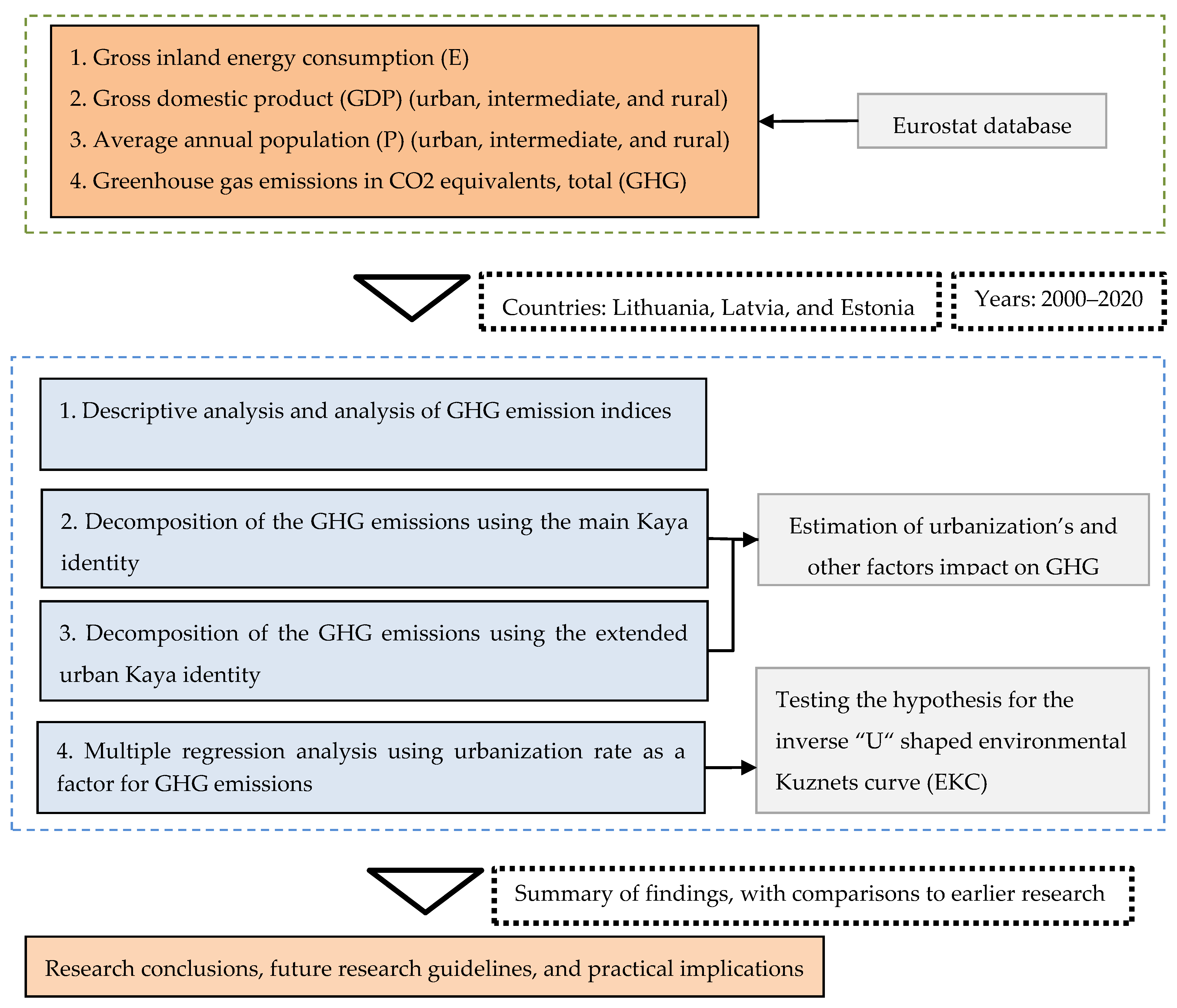
2.1. Data

The research investigates the urban Kaya identity as well as the existence of the EKC in the Baltic States. More specifically, the research emphasises the rate of urbanisation in all three Baltic States and its relationship with environmental degradation. The research employs GHG emissions in CO2 eq (total, excluding LULUCF and memo items) as a proxy for environmental degradation. In addition, the study uses data on total energy consumption (measured in thousands of metric tonnes of oil equivalents), GDP, and total population, which is split into urban, intermediate, and rural populations. The research examines annual statistics from 2000 to 2020. Eurostat databases are used to gather data on all selected indicators [5,6,7]. To compare the economic outcomes of various nations, the gross value added is analysed in purchasing power parities (PPP) at the current prices for each year.
Eurostat identifies three types of regions based on the share of the rural population: (i) predominantly urban regions (rural population: <20% of the total population); (ii) intermediate regions (rural population: 20–50% of the total population); (iii) predominantly rural regions (rural population: >50% of the total population) [43]. According to this typology, Eurostat provides population and GDP statistics.

2.2. Research Framework

The research is divided into several steps: (1) All three states’ descriptive data for indicators are provided and analysed; (2) Decomposition of the GHG emissions using the main Kaya identity is performed; (3) Decomposition of the GHG emissions using the extended urban Kaya identity is performed; (4) A multiple regression analysis using urbanisation rate as a factor for GHG emissions is performed. This allows for an estimate of urbanisation’s and other factors impact on GHG in all three Baltic States in the years 2000–2020 as well as to test the hypothesis for the inverse U-shaped EKC. Next, we provide the study’s research framework (see Figure 1).

2.3. Decomposition of the GHG Emissions Using the Main Kaya Identity

The Kaya identity, first proposed by Yoichi Kaya in 1989 [44], is used to describe the effects on the environment and evaluate the importance of crucial elements influencing changes in GHG emissions. The original (main) Kaya identity can be seen in Formula (1). This consists of four factors—the energy GHG emission coefficient (GHG/E), the energy use intensity (E/GDP), GDP per capita (GDP/P), and total population (P).
G H G = G H G E × E G D P × G D P P × P
where: GHG is total greenhouse gas emissions; E is total energy consumption; GDP is gross domestic product; and P is total population.
Decomposition using the Kaya identity is based on LMDI methods. The two types of LMDI decomposition are additive and multiplicative [45]. The additive GHG emissions contribution from each factor in the main Kaya is estimated using Formula (2).
Δ G H G x = G H G t G H G t 1 ln G H G t ln G H G t 1 × ln x t x t 1
where: GHG is the total greenhouse gas emission; x is the variable in the Kaya identity; Δ is the difference of the first level; t is the time period; t − 1 is the previous time period; and ln is the natural log.
The multiplicative GHG contribution from each factor in the main Kaya model is estimated using Formula (3).
D x = x t x t 1
where: D is the multiplicative effect; x is the variable in the Kaya identity; t is the time period; and t − 1 is the previous time period.

2.4. Decomposition of the GHG Emissions Using the Extended Urban Kaya Identity

The article focuses on urban–rural typology statistics to identify the dynamics of the urbanisation process in the three Baltic States and its impact on environmental degradation. Using the urban–rural typology statistics, GDP per capita consists of gross value-added domestic product produced in urban, intermediate, and rural areas (Formula (4)). The coefficient U stands for the rate of urbanisation in each country and is measured as the percent of the total population living in urban, intermediate, and rural territories.
G D P P = G D P U P U × U U + G D P I P I × U I + G D P R P R × U R
where: G D P is gross domestic product; P is total population; U is the rate of urbanisation; G D P U is total GDP created in urban areas; G D P I is total GDP created in intermediate areas; G D P R is total GDP created in rural areas; P U is population in urban areas; P I is population in intermediate areas; and P R is population in rural areas.
Other authors’ studies extended the original Kaya identity by including more factors or breaking these factors down into components [29]. The urban Kaya identity is often used by adding urbanisation to the original Kaya identity [46]. In our study, the extended urban Kaya identity can be seen in Formula (5). This consists of the abovementioned factors: GDP and population in different areas, as well as urbanisation rates.
G H G = G H G E × E G D P × G D P U P U × U U + G D P I P I × U I + G D P R P R × U R × P U + P I + P R
where: G H G is the total greenhouse gas emission; other variables are described in Formulas (1) and (4).
Once the decomposition of GHG emissions using the abovementioned urban Kaya identity is performed, the individual effects of each factor can be estimated. This is also measured by using both additive ( Δ ) and multiplicative ( D ) effects.
The additive contribution from urban GDP can be seen in Formula (6). In such a manner, it is also possible to calculate intermediate Δ G H G i n t e r m e d i a t e and rural Δ G H G r u r a l additive effects. Then, using Formula (2) effects from GDP/P and urbanisation rate (U) can be separated according to the typology (urban, intermediate, and rural). Using this dependence, it is also possible to decompose the population effects Δ P into urban Δ P u r b a n , intermediate Δ P i n t e r m e d i a t e , and rural areas Δ P r u r a l .
Δ G H G u r b a n = Δ G H G × Δ U U × G D P U P U Δ G D P P
where: G H G is the total greenhouse gas emission; G D P is the gross domestic product; P is the total population; U U is the rate of urbanisation; G D P U is the total GDP created in urban areas; P U is the population in urban areas; Δ is the difference of the first level.
The multiplicative contribution from urban GDP can be seen in Formula (7). Calculating the intermediate D i n t e r m e d i a t e and rural D r u r a l multiplicative contributions is also achievable in this way. Then, using Formula (3), effects from GDP/P and urbanisation (U) can be separated according to the typology (urban, intermediate, and rural).
D u r b a n = G H G t G H G t 1 Δ U U × G D P U P U Δ G D P P
where: D is the multiplicative effect; G D P is the gross domestic product; P is the total population; U U is the rate of urbanisation; G D P U is the total GDP created in urban areas; P U is the population in urban areas; t is the time period; t 1 is the previous time period; Δ is the difference of the first level.

2.5. Multiple Regression Analysis Using Urbanisation Rate as a Factor for GHG Emissions

The econometric equation for the EKC relationship test can be seen in Formula (8). We define this equation similarly to other authors [47] and expect parameters β 1 > 0 and β 2 < 0 to validate the inverse U-shaped relationship between economic growth and environmental degradation. In addition, time dummy variables are used to describe the Baltic States’ accession to the European Union in 2004, as well as the financial crisis of 2009 and the COVID-19 pandemic years of 2020, as all these key years played a significant role in countries’ economies and their applied green policies. If time dummy variables are observed to be statistically insignificant ρ > 0.05 , they are eliminated from the model.
ln G H G P = β 0 + β 1 ln G D P P + β 2 ln G D P P 2 + β 3 D 2009 + β 4 S 2004 + β 5 D 2020 + ε
where: G H G is the total greenhouse gas emission; P is the total population; G D P is the gross domestic product; ε is the error; D 2009 is a time dummy variable (if the year is 2009, the value is 1, otherwise it is 0); S 2004 is a dummy variable (if the year is 2004 or later, the value is 1, otherwise it is 0); D 2020 is a time dummy variable (if the year is 2020, the value is 1, otherwise it is 0); β 0 , 1 , 2 , 3 , 4 , 5   are model parameters; and l n is the natural log.
An expanded econometric equation for the EKC relationship test using urbanisation rate as the proxy for economic growth can be seen in Formula (9). This equation uses more variables. Therefore, we use the procedure of sequential elimination of variables using the software Gretl until all parameters have a two-sided p-value of 0.05.
ln G H G P = β 0 + β 1 ln G D P P + β 2 ln G D P P 2 + β 1 ln U U + β 2 ln U U 2 + β 3 D 2009 + β 4 S 2004 + β 5 D 2020 + β 6 ln U U + β 7 ln U U 2 + ε
where: U U is the rate of urbanisation; other variables are described in Formula (8).
After constructing models best describing the relationship between economic growth and environmental degradation, we provide their determination coefficient R 2 values as well as the results for a test of the model’s normality of residuals using the Doornik–Hansen test (n-test) and a test for heteroskedasticity, the Breusch–Pagan test (BP-test). The study also uses panel data (time series) for all three Baltic States. In this case, we also apply the Pesaran CD test for cross-sectional dependence.

3. Results

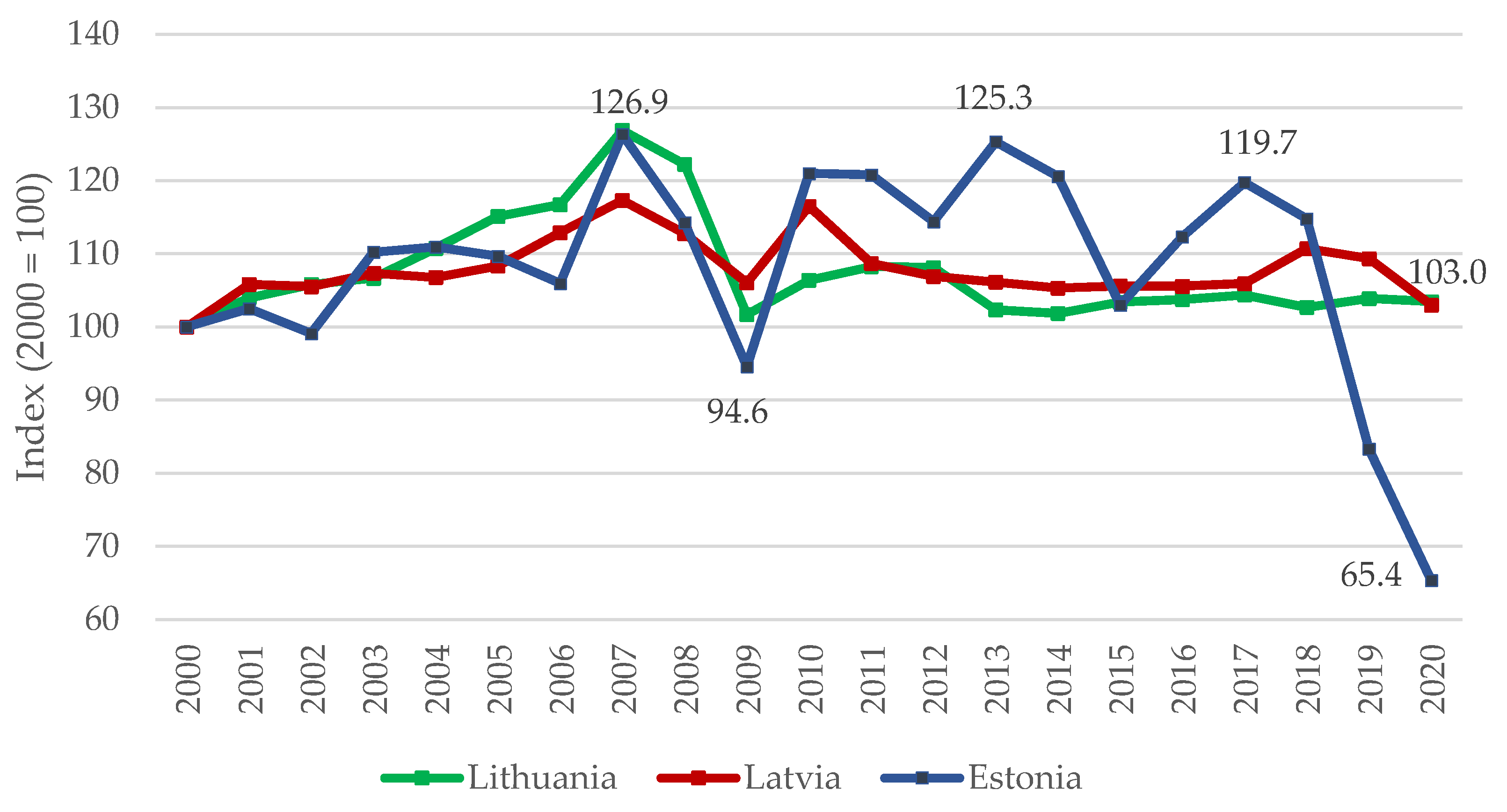
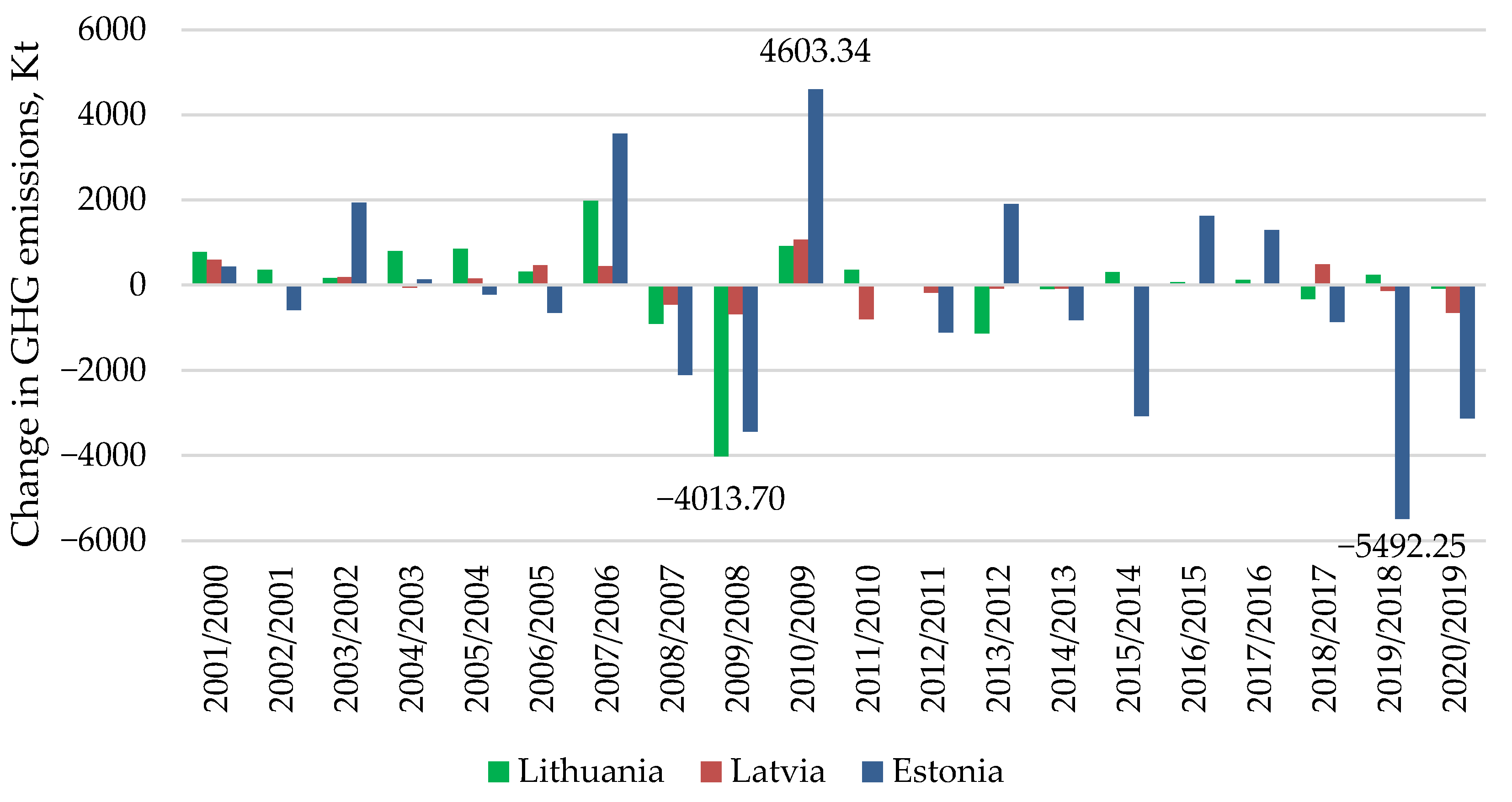
3.1. Descriptive Analysis and Analysis of GHG Emission Indices

Figure 2 depicts the dynamics of GHG emissions in the Baltic States from 2000 to 2020. Latvia and Lithuania are estimated to have similar dynamics of GHG emissions, with Lithuania and Latvia having about 103% of the initial 2000 level in 2020. Lithuania reached a peak in 2007, reaching 126.9% of the initial GHG emission value. Latvia reached its peak in 2010, reaching 121.0% of the initial GHG emission value. GHG emissions in Estonia have changed more dramatically between the years 2000 and 2020. GHG emissions in Estonia fell by up to 94.6% in 2009 and even more in 2020, to 65.4%. In Estonia, GHG emissions peaked in 2013 at 125.3% of the initial level.
Figure 3 depicts changes in GHG emissions across all three Baltic countries from 2000 to 2020. Estonia has had the most dramatic changes in GHG emissions, increasing GHG emissions by 4603.3 Kt of CO2 eq in 2010. However, Estonia’s GHG emissions decreased by 5492.3 Kt of CO2 eq in 2019. GHG emissions in Lithuania remained relatively stable. However, there was a significant fall in 2009, when GHG emissions were reduced by 4013.7 Kt of CO2 eq. GHG emissions increased the most in Lithuania in 2007 by 1979.9 Kt of CO2 eq. The changes in GHG emissions in Latvia were the smallest: the largest reduction was in 2011 by 796.9 Kt of CO2 eq, and the largest increase was in 2010 by 1066.7 Kt of CO2 eq.
The descriptive statistics of all four indicators in the main Kaya identity can be seen in Table 1. The GHG emissions were largest in Lithuania, where the mean in the years 2000–2020 is estimated to be 20,999.6 Kt of CO2 eq, and least in Latvia, where the mean is estimated to be 10,999.8 Kt of CO2 eq. As mentioned above, the GHG emissions were most volatile in Estonia (13.432% mean value) and least volatile in Latvia (3.869% mean value). The GHG/E, E/GDP, and GDP/P are largest on average in Estonia and smallest in Latvia. During these years, Lithuania had the largest population, whereas Estonia had the smallest population.
The structure of energy use is provided in Figure A1. In Lithuania, oil and petroleum products contribute to more than 50% of the energy balance. In Latvia, oil and petroleum products contribute to around one-third of the energy balance. Finally, in Estonia, a large share of the energy balance comes from other sources, most notably nuclear heat (until 2010) and electricity.

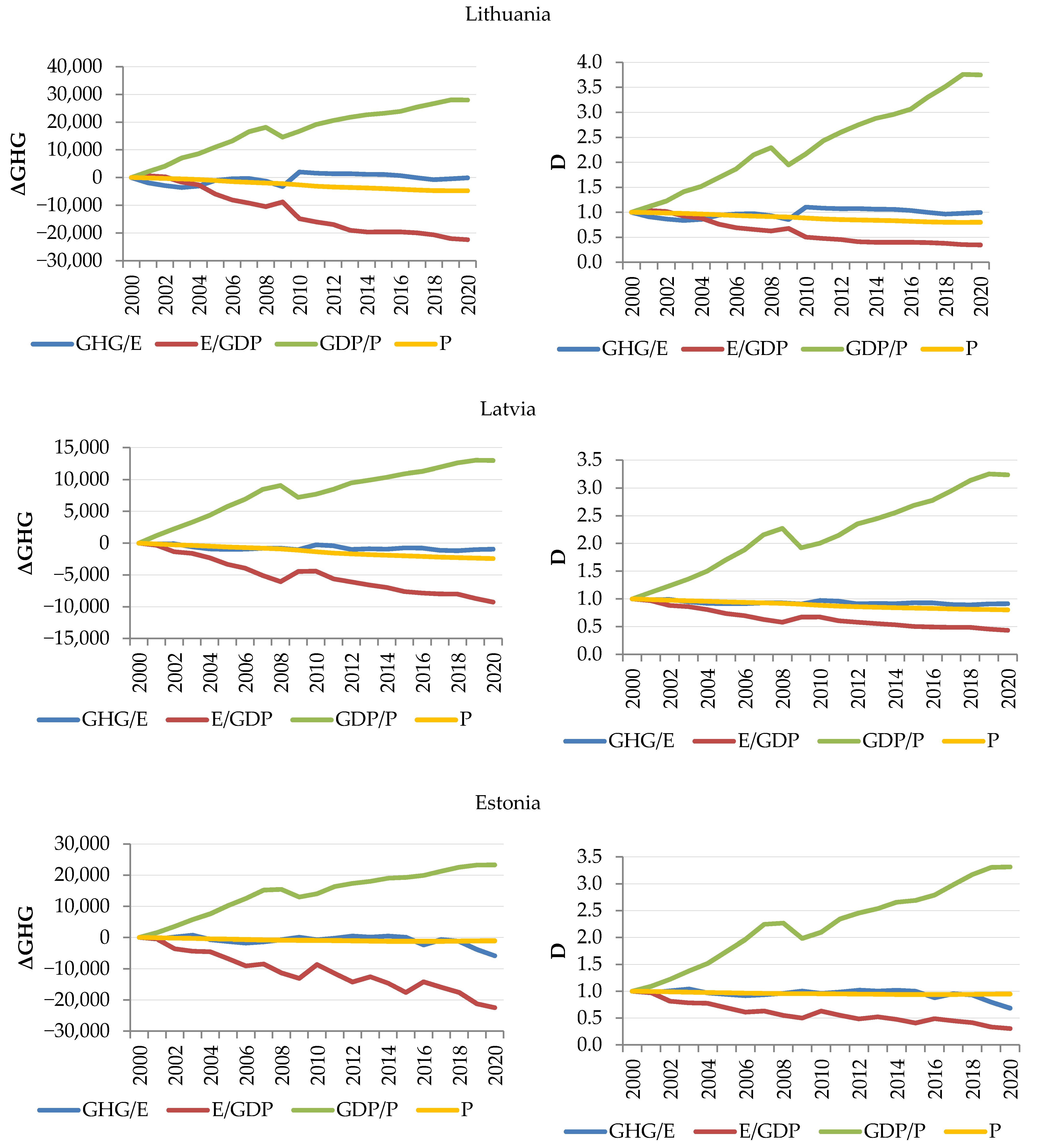
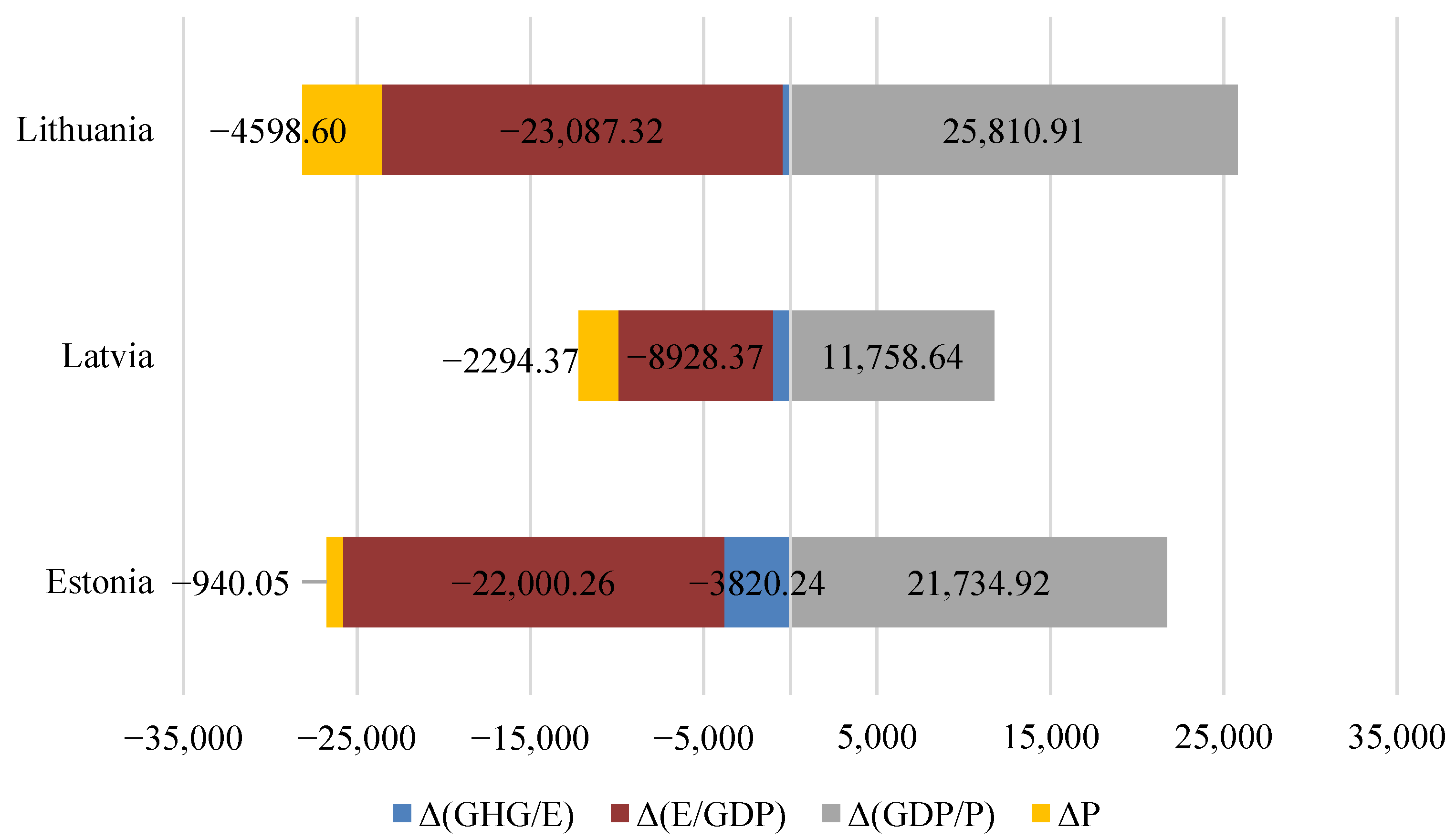
3.2. Estimates from the Main Kaya Identity

Next, we apply the Kaya identity to estimate the effects of different factors (GHG/E, E/GDP, GDP/P, and P) on GHG emissions. A graphic depiction of additive factors in the Kaya identity can be seen in Figure A2.
Next, we provide both additive and multiplicative effects by accumulating them throughout the years 2000–2020 (see Figure 4). Here we can see that in Estonia, GHG/E remained relatively stable, but in Lithuania and Latvia, it increased after the year 2009. E/GDP, regardless of fluctuations, decreased in all three countries. GDP/P increased in all three countries except for the global financial crisis in 2009 and the pandemic period in 2020. The effect of P remained relatively stable but steadily decreased in all three countries.
Next, the structure of cumulative effects from the final year of 2020 used in the study is displayed in Figure 5. Here we can see that GHG/E had only a small but negative effect on GHG in all three countries: the largest in Estonia (−3820.2), then in Latvia (−1000.8), and finally in Lithuania (−469.2). E/GDP greatly reduced GHG emissions in all three countries: the reduction was the largest in Lithuania (−23,087.3), then in Estonia (−22,000.3), and smallest in Latvia (−8928.4). Growing GDP/P increased GHG emissions in all three countries: the increase was the largest in Lithuania (25,810.9), then in Estonia (21,734.9), and the smallest in Latvia (11,758.6.6). P had a relatively small effect on GHG emissions, but it decreased them in all three countries: the reduction was the largest in Lithuania (−4598.6), then in Latvia (−2294.4), and the smallest in Estonia (−940.1).

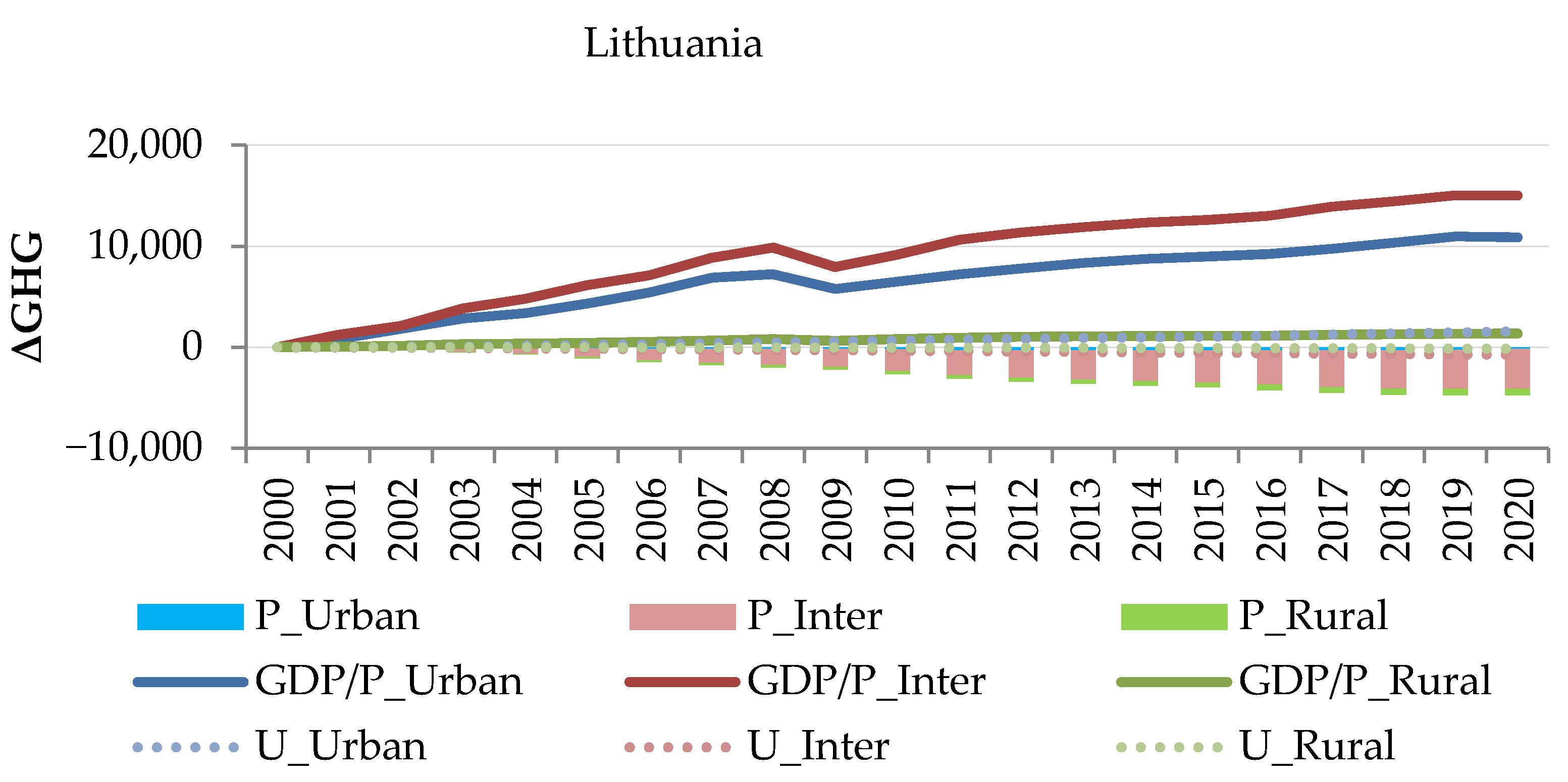
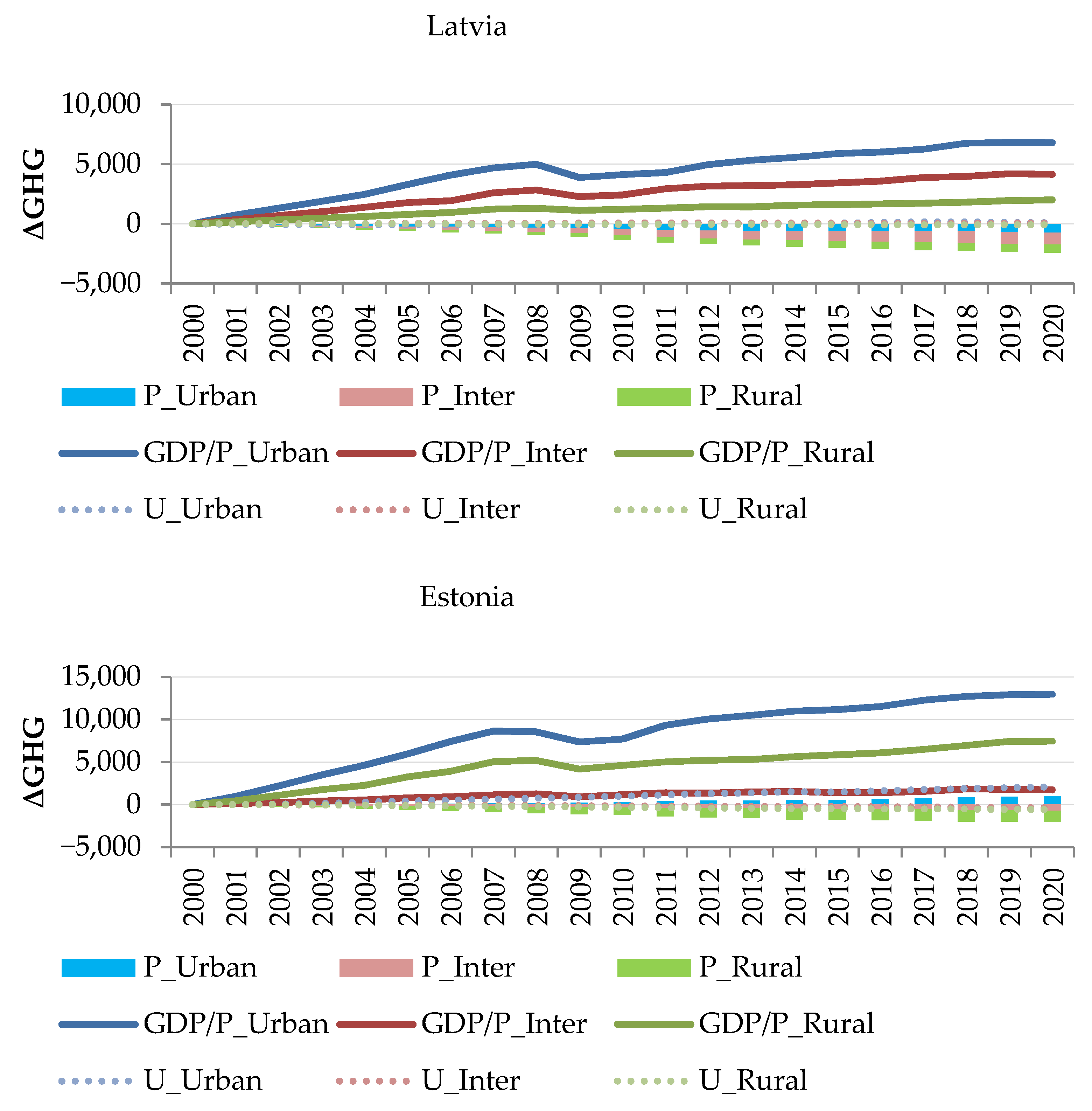
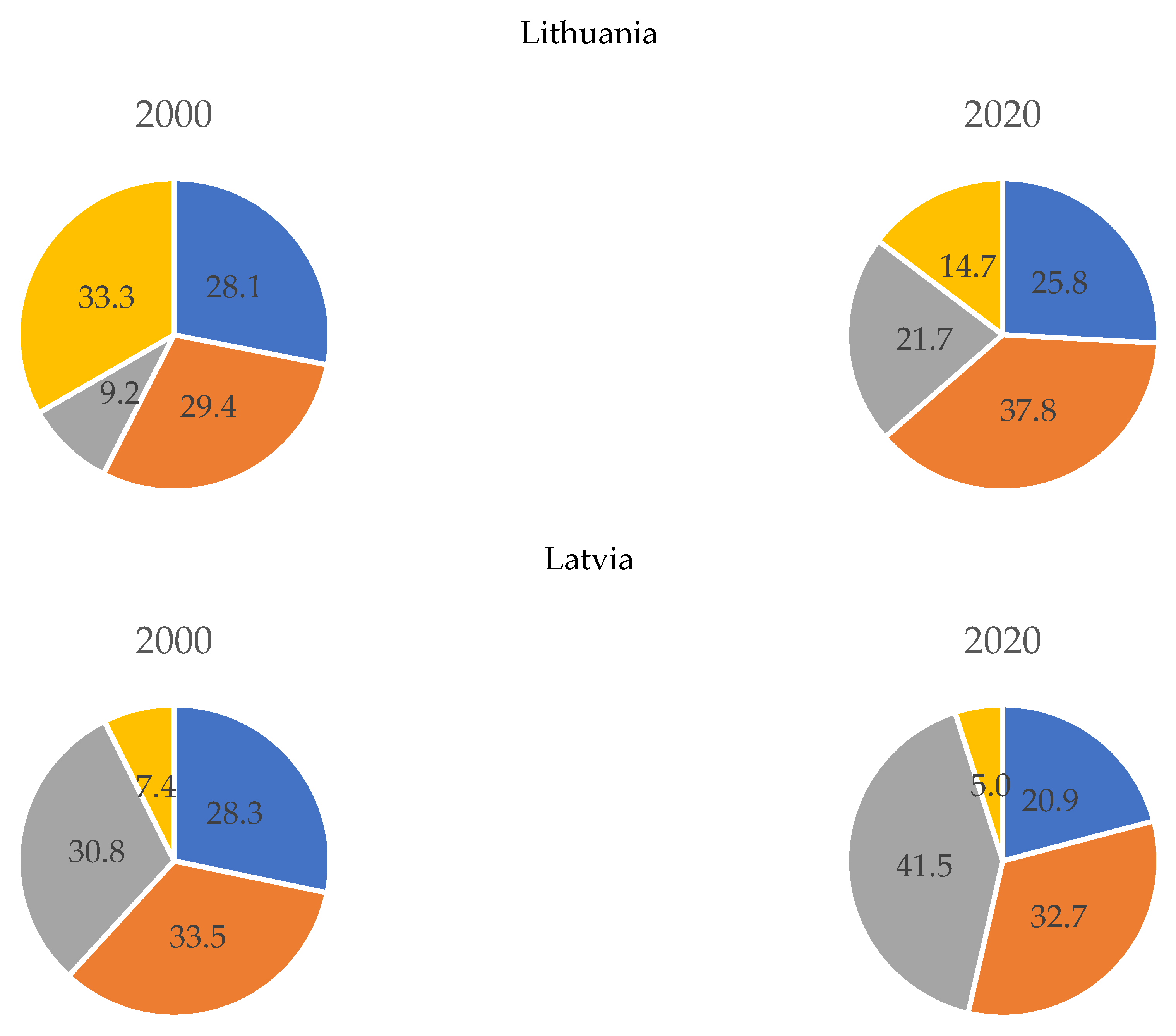
3.3. Estimates from the Extended Urban Kaya Identity

The estimates of urbanisation rates’ multiplicative and additive effects are then provided (see Table 2). Note that UU reflects the proportion of the total population living in urban areas, UI in intermediate areas, and UR in rural areas. Positive changes in the UU rate had the greatest impact in Lithuania in 2016–2017, when GHG emissions increased by 0.57%, or 115.6 Kt. The years 2000–2001 witnessed the smallest increase in the component indicated previously (13.7 Kt), which corresponds to a 0.07% increase in GHG emissions. In 2015–2016, the UU had the largest impact in Latvia (55.4 Kt, or 0.52%). The largest decline in Latvia was observed between 2019 and 2020 and was estimated to be 0.39% (−42.8 Kt). The UU rate in Estonia had the greatest impact between 2010 and 2011, when GHG emissions increased by 0.77%, or 162.6 Kt, whereas the largest decline was between 2014 and 2015 (−28.3 Kt), which amounted to 0.15%. The effects of UI in Lithuania are estimated to be negative during all years used in the study. The greatest negative impact of intermediate UI was discovered in Lithuania in 2016–2017, accounting for 0.24% (−49.6 Kt). The smallest decline that occurred between 2000 and 2001 (−11.3 Kt) is estimated to have been 0.06%. In 2019–2020, the UI had the greatest positive impact in Latvia (18.0 Kt), with an estimated increase of 0.17%. The years 2015–2016 saw the greatest decline, which can be calculated to be 0.11% (−11.6 Kt). In 2014–2015, the UI rate had the smallest negative impact in Estonia (−6.7 tonnes, or 0.03%). The largest decline in Estonia was observed between 2017 and 2018 (−59.3 Kt), representing 0.29%. In 2000–2001, UR had an estimated 0.01% (1.7 Kt) influence on the GHG emissions in Lithuania. Between 2019 and 2020, there was a reduction of 15.9 Kt, or 0.08%. In 2000–2001, the impact of the UR rate was 0.02% in Latvia (2.2 Kt). The decline from 2016 to 2017 (−11.4 Kt) represented 0.11%. In Estonia, the UR rate had the greatest impact in 2014–2015, accounting for 0.1% (19.8 Kt). The largest decline of UR in Estonia was observed between 2010 and 2011 (−52.3 Kt), which was 0.25%.
Next, the estimates of the additive and multiplicative effects of factor GDP/P are given (see Table 3). In Lithuania, the largest impact of the growing urban GDP/P factor was discovered in 2006–2007 (1457.9 Kt) and can be estimated to have increased GHG by 6.33%. These were the years of the economic boom prior to the economic crisis of 2008–2009. The largest decreasing effect from the previously mentioned factor was observed in the financial crisis years of 2008–2009 (−1450.4 Kt) and can be estimated to have reduced the GHG emissions by 6.44%. In Latvia, the largest impact of the urban GDP/P factor was discovered in 2004–2005 (821.2 Kt, or 7.78%). These were the years of Latvia’s accession to the European Union. The largest decrease was observed in the years 2008–2009 (−1113.6 Kt) and can be estimated to be 9.51%. In Estonia, the largest impact of the urban GDP/P factor was discovered in 2010–2011 (1617.6 Kt) and can be estimated to have increased GHG emissions by 7.97%. These are the years after the economic crisis of 2008–2009. The largest decrease was observed in the years 2008–2009 (−1157.5 Kt) and can be estimated to be 6.17%. The effects caused by the intermediate GDP/P factor are larger than those caused by urban GDP/P in Lithuania. In Lithuania, the largest impact of the intermediate factor was discovered in 2002–2003 (1724.8 Kt) and can be estimated at 8.67%. The largest decrease was observed in the years 2008–2009 (−1922.2 Kt), and it can be estimated to be 8.44%. In Latvia, the largest impact of the intermediate segment was discovered in 2006–2007 (675.9 Kt) and can be estimated at 5.93%. The largest decrease in Latvia was observed in the years 2008–2009 (−560.9 Kt), and it can be estimated to be 4.91%. Note that GDP is measured in purchasing power parities (PPP), so the impact of price levels is eliminated. In Estonia, the largest impact of the intermediate GDP/P factor was discovered in 2017–2018 (277.6 Kt, or 1.37%). The largest decrease was observed in the years 2008–2009 (−335.6 Kt) and can be estimated to be 1.83%. When analysing the rural GDP/P factor in Lithuania, the largest impact of rural GDP/P was discovered in 2002–2003 (171.5 Kt) and can be estimated at 0.83%, whereas the largest decrease in Lithuania was observed in the years 2008–2009 (−188.0 Kt) and can be estimated to be 0.86%. In Latvia, the largest impact of rural GDP/P was discovered in 2006–2007 (282.7 Kt) and can be estimated at 2.44%. The largest decrease in Latvia was observed in the years 2008–2009 (−182.6 Kt) and can be estimated to be 1.62%. In Estonia, the largest impact of rural GDP/P was discovered in 2004–2005 (994.0 Kt) and can be estimated at 5.3%. The largest decrease was observed in the years 2008–2009 (−1011.0 Kt) and can be estimated to be 5.41%. Note that for all three Baltic States in 2019–2020, different contributing factors differed in their signs: rural GDP/P increased GHG, whereas urban and intermediate GHG decreased it.
Following that, assessments of additive and multiplicative effects from the total population living in urban, intermediate, and rural areas are provided (see Table 4). In most years in Lithuania, the declining urban population has a negative impact on GHG emissions. The greatest positive rise was found in the years 2019–2020 (70.4 Kt), with an estimated 0.35% gain. The most significant negative impact of urban population was identified in 2010–2011 (−62.5 Kt) and is estimated to be 0.3%. The greatest positive impact of urban population growth was observed in Latvia in 2015–2016 (1.1 Kt) and is estimated to be 0.01%. The greatest reduction (−75.9 Kt) was observed in 2009–2010 and is assessed to be 0.67%. The biggest positive impact of the urban population in Estonia was observed in 2017–2018 (112.6 Kt) and is assessed to be 0.55%. The greatest reduction (−34.9 Kt) was reported in the years 2000–2001 and is assessed to be 0.2%. In Lithuania, the intermediate impacts are larger than the urban effects throughout the majority of the years. In Lithuania, all intermediate population impacts are negative. The greatest negative impact of the intermediate was discovered in Lithuania in 2010–2011 (−361.1 Kt) and is assessed to be 1.71%. The smallest negative impact (−38.4 Kt) was found in 2019–2020, and it is predicted to be 0.19%. The greatest negative impact of the intermediate was discovered in Latvia in 2009–2010 (−96.1 Kt) and is assessed to be 0.84%. The smallest negative impact (−6.5 Kt) was found in 2019–2020, and it is predicted to be 0.06%. The highest negative impact of the intermediate was discovered in Estonia in 2017–2018 (−87.2 Kt) and is assessed to be 0.43%. The smallest negative impact (−12.4 Kt) was seen in 2014–2015, and it is assessed to be 0.06%. In Lithuania, all rural population effects are negative. The greatest negative impact of rural population was identified in Lithuania in 2010–2011 (−49.6 Kt) and is estimated to be 0.24%. The smallest negative impact (−12.5 Kt) was seen in the years 2000–2001, and it is assessed to be 0.06%. The greatest detrimental impact of the intermediate was discovered in Latvia in 2009–2010 (−66.8 Kt) and is assessed to be 0.59%. The smallest negative impact (−14.3 Kt) was found in 2019–2020, and it is predicted to be 0.13%. The biggest positive impact of the intermediate was discovered in Estonia in 2017–2018 (28.9 Kt) and is assessed to be 0.14%. The greatest negative impact was found in 2003–2004 (−132.1 Kt), with an estimated 0.68%.

3.4. Estimates from the U-Kuznet’s Curve Model

Next, the statistical estimates of the EKC are provided using both approaches (see Table 5). We use the OLS method to estimate the parameter values in each model. We begin with the model using GDP/P and (GDP/P)2 as the independent variables to explain GHG/P. Statistically significant effects are found in all three countries except for Latvia, where only GDP/P has a p-value below 0.05. In all three countries, (GDP/P)2 has a negative coefficient value, thus providing evidence for the hypothesis of the inverse U-relationship between GHG/P and economic growth, but it can only be accepted in Lithuania and Estonia. Another important observation is that in Lithuania and Estonia, the dummy variable indicating the year 2009 of the financial crisis is statistically significant and reduces GHG. In Estonia, the dummy variable indicating the COVID-19 pandemic in 2020 also has a statistically significant negative effect on GHG/P. When analysing panel data for all three countries, the accession to the EU in 2004 was found to reduce GHG in all three countries.
Then, we analyse models that include coefficients for urbanisation (UU and UU2) to explain GHG/P. After omitting statistically insignificant variables, the urbanisation rate is found to increase GHG/P in Lithuania and reduce it in Estonia. However, there is no evidence of an inverse U-relationship between these variables. Another important observation is that in Estonia, the urbanisation rate explains GHG/P better than GDP/P as GDP/P is omitted from the model as statistically insignificant. All models using urbanisation rates have residual normality test p-values above 0.05, showing that the residuals are normally distributed. However, only the model for Lithuania has heteroscedasticity test results with p above 0.05, showing that homoscedasticity among residuals is present. The cross-sectional dependence test indicates a p-value above 0.05, showing that there is a weak cross-dependence among variable time series.

4. Discussion

4.1. Comparison with Previous Studies

In the study, the Kaya identity was applied to analyse GHG emissions and their constituent components. The extended Kaya method was also widely applied in the analysis of carbon emissions and various aspects of urbanisation by other authors in different countries: energy efficiency by various sources [49], fossil fuel type [50], urbanisation effects [51], household energy consumption [52], agriculture sector [53]. Our study focuses on the effects of urbanisation ratio, urban population, and urban economic growth on GHG emissions. The research conducted, established the following main points:
First, according to Kaya’s estimates, GDP per capita growth has the largest and most positive effect on GHG emissions in all three countries. The second-largest effect is from energy intensity, which decreased in all three countries, as did GHG emissions. The remaining two effects (gas emission coefficient and population) both have relatively small effects.
According to other authors, who also used the LMDI to disaggregate CO2 emissions in terms of the type of fuel source, rapid economic growth is the main contributing factor in developing countries, whereas energy intensity reduces CO2 [20]. For example, energy intensity had a balancing effect on carbon emissions, which decreased them even if per capita GDP increased in China [21]. Population, energy intensity, and GDP per capita are the three factors with the most influence, whereas the carbon emission coefficient has the least, according to a global perspective [22]. According to the findings, while population and gross domestic product (GDP) per capita are on the rise, energy intensity and carbon intensity are on the decline [19]. The G7 group of rich nations’ reduced carbon dioxide emissions appeared to be mostly driven by energy intensity [23]. Lower-middle-income countries have a decrease in CO2 emissions as a result of the energy intensity effect, whereas upper-middle and high-income countries experience an increase that may both raise and lower the overall level of CO2 emissions [24]. According to a Kaya identity decomposition, the rise in GDP was the primary driver of the EU’s territorial emissions prior to the global financial crisis [54]. The findings of Kaya Identity showed that a rising population, rising GDP per capita, and declining energy efficiency were the main factors causing CO2 emissions to rise in South Africa [25]. The disparity between the regions, however, dramatically widened, and the GDP per capita has a greater impact on the amount of emissions compared to the population as a driving element [27]. Similarly, other authors’ research showed that despite annual variations in energy intensity and economic development, these two factors had the biggest effects on changes in GHG emissions in Baltic countries [28]. Authors also revealed that GHG emissions decreased in Baltic countries as a result of increases in labour productivity, decreases in the share of fossil fuels, and increases in the number of employees and emissions intensity [55]. Authors analysing Latvian data discovered that energy efficiency and the proportion of fossil fuel consumption in total may only change the direction of GHG emission reduction [26].
The second important discovery includes the effects of urbanisation. It was found that population changes in urban areas reduced GHG while the GDP per capita produced there increased. On the other hand, an exception was found in Estonia, where both population and GDP per capita increased GHG emissions. In this study, all countries increased their urbanisation rates, but the increase was largest in Estonia.
The urbanisation topic is still under research in the Baltic countries, but according to the findings from other countries, the urbanisation effect continues to have a significant impact on overall carbon emissions [29]. Urbanisation plays an important role in GHG emissions, especially in developing countries such as China [30]. Contrary to expectations, major population shifts from rural to urban areas led to an increase in household GHG footprints in emerging regions, with >1% increases in China, Indonesia, India, and Mexico over the period [31]. According to other authors’ findings, higher rates of urbanisation, energy carbon emission coefficients, and energy intensities will result in larger carbon emissions [32]. However, greater than population growth and urbanisation rates, GDP per capita contributes more to CO2 emissions, and this contribution rate is rising [33]. Other authors also emphasise that the socioeconomic elements of economic expansion, urbanisation, and industrialisation will result in more CO2 emissions, while advancements in service and technology levels may result in lower CO2 emissions [30]. The outcome also showed that economic expansion has a favourable and significant effect on carbon emissions, suggesting that economic growth directly lowers environmental quality through raising carbon emissions in highly urbanised Singapore [9]. Other authors reveal that energy intensity is the main factor in urban–rural CO2 emission inequality [56].
The final observation in this study is that there is some evidence for an EKC in Estonia and Lithuania, but only when using the GDP as an indicator for economic growth. The inverted U-shaped EKC hypothesis is typically disproven in the Baltic countries, according to the findings of other econometric research [57], or only in Lithuania [58]. The hypothesis is valid when analysing pooled data from the Baltic and Visegrad countries [59]. Other authors who examined Lithuanian data discovered that the growth in the intensity of renewable resources and energy efficiency, as well as the decline in GHG, were all influenced by the drop in energy consumption and the decarbonisation index [60]. The authors analysed the EKC in other countries: Japan [40], the USA [61], South Africa [62], Saudi Arabia [63], and Singapore [9]. The EKC is typically observed in studies that include higher-income countries. Our study also used the urbanisation ratio as a factor for GHG emissions in the EKC model. Similarly, to other authors who analysed different countries, the relationship between urbanisation and CO2 emissions is positive but not curved [35,37]. Other authors reveal that when urbanisation increases beyond a certain level, it does not stimulate higher CO2 [39,41]. Others reveal that urbanisation’s impact on environmental degradation varies across different economic regions [34].

4.2. Limitations and Proposals for Future Research

The study uses the LMDI to decompose the extended Kaya model. The study emphasizes the effects of urbanisation on GHG emissions in the Baltic States. Index decomposition analysis (IDA) methods, such as Kaya identity, are used by other authors not only in the investigation of national but also regional and sectoral changes in carbon emissions to separate these from economic or population growth [64], for example, in the commercial building sector [65,66,67,68] and industrial sectors [69]. Therefore, future research can focus on agriculture or another sector that produces most of the GHG in the Baltic countries. Another important aspect of future research is to separate GHG according to different source types. For example, according to other authors, relative (weak) decoupling in the Baltic states of the relationship between transport-related GHG emissions and economic growth was found [70].
Some authors claim that larger cities emit fewer GHG emissions than smaller ones [71]. Therefore, the further analysis of urbanisation effects can be more detailed according to the structure of cities and their size in the Baltic States.
The study could analyse more countries. A future study can also use more sophisticated time series methods. For example, a quantile regression approach can be used to assess the drivers of carbon emission from production activities at different quantile levels, employing an augmented Kaya identity, similar to other authors [72]. The correlation between Kaya identity factors and their decomposed variables can also be analysed [73]. The research can include the modified Kaya identity in the autoregressive distributive lag model (ARDL), which is a time series approach [74]. A multivariate co-integration analysis of the Kaya factors can be performed [75]. To predict the carbon footprint and investigate the effects of the energy consumption paradigm shift policy, simulations can be run [76]. Multi-criteria decision-making (MCDM) and MULTIMOORA can also be applied [77]. Convergence processes for several groups of EU countries can be applied [78]. For example, other authors have analysed convergence processes in South America [79].
The main limitation of this study is that the data was only available up to 2020 during the study. Research employed time dummy variables such as the global financial crisis and countries’ accession to the EU. Once more data becomes available, the research can also emphasise the effects of the post-COVID-19 crisis on GHG emissions [80]. Additionally, the study can add more economic development variables to the extended Kaya identity or split GHG emissions and energy use according to fuel type or sector, as currently we are using the total GHG emissions and energy use. Since there is evidence for the inverse U-shaped EKC in Lithuania and Estonia, future research can also dwell on more complex forms of interrelationships between economic growth and environmental degradation, such as the N-shaped EKC.

4.3. Practical Implications

In this study, the three Baltic states were chosen for examination due to their similar economic systems, comparable development levels, and the fact that these countries adopted the EU‘s aim to be climate-neutral by 2050. According to a study by Siksnelyte [77], Denmark and Latvia had the best records in terms of achieving the EU’s development targets for sustainable energy during the study period. Others emphasise growing energy demand in manufacturing and transport sectors for all three Baltic nations [81]. However, the study’s conclusions show that economic growth is insufficient to address environmental problems. The study recommends that the government prioritise carbon reduction initiatives more highly and implement them successfully at the national level.
Other authors propose several strategies to control energy use and GHG emissions, highlighting: carbon removal [82], manufacturing and transportation-related activity [81], policymaking, and societal issues [47], sustained energy efficiency improvement, dramatic industrial reorganisation, and energy transition [83], and improving energy efficiency [84,85], providing adequate technologies and infrastructure in urban areas [86], and renewable energy [87]. Authors who analysed OECD countries discovered that the cornerstones for decarbonisation appear to be activity reduction, energy conservation, renewable electrification, efficient power plants, and the phase-out of coal [88]. However, the primary compensating factor impeding the achievement of greater GHG emission reductions was the impact of economic expansion [89]. Others claim that larger cities emit fewer GHG than smaller ones. This finding points to the need for improved energy production and consumption technologies as well as efficient transportation methods [71]. Improved household solar energy use, particularly among farm households, has been attributed in part to subsidy schemes, while greater heated areas in rural homes and positive attitudes towards renewable energy have also improved self-reported energy bill savings [90].

5. Conclusions

This study examines the relationship between GHG emissions, economic growth, and urbanisation. The study attempts to extend the body of knowledge and provide a more comprehensive explanation of how these connections are formed. The study uses the Baltic States, which are less studied in the works of other authors and uses annual data for all three countries from 2000 to 2020. Since all three countries have similar geographical, economic, and historical backgrounds, the research results for all three countries are comparable and provide new insights. The research uses an extended Kaya identity where GDP and population are further split into urban, intermediate, and rural components. The study also tests the EKC hypothesis using economic growth and urbanisation as factors for GHG emissions.
The study led to three major conclusions. First, in all three countries, GDP per capita growth has the biggest impact on GHG emissions, according to Kaya’s identity decomposition. Energy intensity, which dropped in all three nations along with GHG emissions, has the second-largest impact. Both the population and the gas emission coefficient have relatively small effects on GHG emissions. This finding is similar to the results obtained by other researchers who analysed the Baltic and other countries. Second, it was discovered that changes in the urban population until 2020 decreased GHG emissions in Latvia and Lithuania, as shrinking urban population had a diminishing effect on GHG emissions. However, in Estonia, GHG emissions rose not only from urban GDP per capita growth, but also from an increased urban population. In the time frame analysed, the rates of urbanisation rose fastest in Estonia. The study’s final finding is that the hypothesis on the EKC can be accepted when analysing data from Lithuania and Estonia, but only when using GDP per capita as a factor for GHG emissions. The urbanisation rate has a statistically significant one-directional effect on GHG emissions when analysing Lithuania, Estonia, and panel data. However, in Estonia, this effect is negative, showing that increases in urbanisation rates have a diminishing effect on GHG emissions. However, there is no inverse U-shaped relationship between urbanisation rate and environmental degradation in all three countries.
The data used in the study only goes back to 2000, as only that much data on urban GDP and population was available for all three Baltic countries. Therefore, the study can be expanded with the availability of more post-2021 data once it becomes available. Another important future research guideline is to include more countries and compare results between eastern and western EU countries. The study can also use more indicators showing economic development and energy sources, adding them to the expanded Kaya identity.
The results of the study have important applications for future policymaking regarding economic development and urban planning in order to enhance environmental quality or slow down environmental degradation, while ensuring economic development in the Baltic States in the upcoming decades.

Author Contributions

Conceptualization, D.M. and A.J.S.; methodology, D.M. and A.J.S.; software, A.J.S.; validation, D.M. and A.J.S.; formal analysis, A.J.S.; investigation, A.J.S.; resources, V.M.; data curation, D.M. and A.J.S.; writing—original draft preparation, D.M. and A.J.S.; writing—review and editing, D.M., A.J.S., V.M. and G.G.-Z.; visualization, D.M. and A.J.S.; supervision, D.M. and A.J.S.; funding acquisition, V.M. All authors have read and agreed to the published version of the manuscript.

Funding

This research received no external funding.

Institutional Review Board Statement

Not applicable.

Data Availability Statement

Not applicable.

Conflicts of Interest

The authors declare no conflict of interest in the results.

Appendix A

Figure A1. The annual structure of energy balance. Source: authors’ calculations based on Eurostat [48] data, 2023.
Agriculture 13 01844 g0a1aAgriculture 13 01844 g0a1b

Appendix B

Figure A2. The estimates of additive factors in the Kaya identity. Source: authors’ calculations based on Eurostat [5,6,7,48] data, 2023.
Agriculture 13 01844 g0a2aAgriculture 13 01844 g0a2b

References

  1. Makutėnienė, D.; Staugaitis, A.J.; Makutėnas, V.; Juočiūnienė, D.; Bilan, Y. An Empirical Investigation into Greenhouse Gas Emissions and Agricultural Economic Performance in Baltic Countries: A Non-Linear Framework. Agriculture 2022, 12, 1336. [Google Scholar] [CrossRef]
  2. Eurostat; European Commission. Population by Broad Age Group (cens_21ag). Eurostat. Available online: https://ec.europa.eu/eurostat/databrowser/view/CENS_21AG/default/table?lang=en (accessed on 20 June 2023).
  3. The World Bank. Population, Total. Available online: https://data.worldbank.org/indicator/SP.POP.TOTL?locations=IE&name_desc=true (accessed on 20 June 2023).
  4. Eurostat; European Commission. GDP and Main Components (Output, Expenditure and Income) (Online Data Code: NAMA_10_GDP). Eurostat. Available online: https://ec.europa.eu/eurostat/databrowser/view/NAMA_10_GDP__custom_6960697/default/table?lang=en (accessed on 20 June 2023).
  5. Eurostat; European Commission. Main GDP Aggregates Per Capita (Online Data Code: NAMA_10_PC). Eurostat. Available online: https://ec.europa.eu/eurostat/databrowser/view/NAMA_10_PC/default/table?lang=en (accessed on 20 June 2023).
  6. Eurostat; European Commission. Average Annual Population to Calculate Regional GDP Data (Thousand Persons) by NUTS 3 Regions (Online Data Code: NAMA_10R_3POPGDP). Eurostat. Available online: https://ec.europa.eu/eurostat/databrowser/view/nama_10r_3popgdp/default/table?lang=en (accessed on 20 June 2023).
  7. Eurostat; European Commission. Greenhouse Gas Emissions by Source Sector (Source: EEA) (Online Data Code: ENV_AIR_GGE). Eurostat. Available online: https://ec.europa.eu/eurostat/databrowser/view/env_air_gge/default/table?lang=en (accessed on 20 June 2023).
  8. Cumming, G.S.; Buerkert, A.; Hoffmann, E.M.; Schlecht, E.; von Cramon-Taubadel, S.; Tscharntke, T. Implications of agricultural transitions and urbanisation for ecosystem services. Nature 2014, 515, 50–57. [Google Scholar] [CrossRef]
  9. Ali, H.S.; Abdul-Rahim, A.S.; Ribadu, M.B. Urbanisation and carbon dioxide emissions in Singapore: Evidence from the ARDL approach. Environ. Sci. Pollut. Res. 2017, 24, 1967–1974. [Google Scholar] [CrossRef]
  10. Avtar, R.; Tripathi, S.; Aggarwal, A.K.; Kumar, P. Population–urbanisation–energy nexus: A review. Resources 2019, 8, 136. [Google Scholar] [CrossRef]
  11. Camarero, L.; Oliva, J. Thinking in rural gap: Mobility and social inequalities. Palgrave Commun. 2019, 5, 95. [Google Scholar] [CrossRef]
  12. Young, A. Inequality, the urban-rural gap, and migration. Q. J. Econ. 2013, 128, 1727–1785. [Google Scholar] [CrossRef]
  13. Ranscombe, P. Rural areas at risk during COVID-19 pandemic. Lancet Infect. Dis. 2020, 20, 545. [Google Scholar] [CrossRef]
  14. Surya, B.; Ahmad, D.N.A.; Sakti, H.H.; Sahban, H. Land use change, spatial interaction, and sustainable development in the metropolitan urban areas, South Sulawesi Province, Indonesia. Land 2020, 9, 95. [Google Scholar] [CrossRef]
  15. Rana, I.A.; Routray, J.K.; Younas, Z.I. Spatiotemporal dynamics of development inequalities in Lahore City Region, Pakistan. Cities 2020, 96, 102418. [Google Scholar] [CrossRef]
  16. Penco, L.; Ivaldi, E.; Bruzzi, C.; Musso, E. Knowledge-based urban environments and entrepreneurship: Inside EU cities. Cities 2020, 96, 102443. [Google Scholar] [CrossRef]
  17. World Cities Report 2022: Envisaging the Future of Cities. United Nations Human Settlements Programme. 2022. Available online: https://unhabitat.org/sites/default/files/2022/06/wcr_2022.pdf (accessed on 25 June 2023).
  18. Yu, X.; Wu, Z.; Zheng, H.; Li, M.; Tan, T. How urban agglomeration improve the emission efficiency? A spatial econometric analysis of the Yangtze River Delta urban agglomeration in China. J. Environ. Manag. 2020, 260, 110061. [Google Scholar] [CrossRef]
  19. Tavakoli, A. How precisely “kaya identity” can estimate GHG emissions: A global review. Jordan J. Earth Environ. Sci. 2017, 8, 91–96. [Google Scholar]
  20. Ortega-Ruiz, G.; Mena-Nieto, A.; García-Ramos, J.E. Is India on the right pathway to reduce CO2 emissions? Decomposing an enlarged Kaya identity using the LMDI method for the period 1990–2016. Sci. Total Environ. 2020, 737, 139638. [Google Scholar] [CrossRef] [PubMed]
  21. Yang, P.; Liang, X.; Drohan, P.J. Using Kaya and LMDI models to analyze carbon emissions from the energy consumption in China. Environ. Sci. Pollut. Res. 2020, 27, 26495–26501. [Google Scholar] [CrossRef]
  22. Tavakoli, A. A journey among top ten emitter country, decomposition of “Kaya Identity”. Sustain. Cities Soc. 2018, 38, 254–264. [Google Scholar] [CrossRef]
  23. Su, W.; Wang, Y.; Streimikiene, D.; Balezentis, T.; Zhang, C. Carbon dioxide emission decomposition along the gradient of economic development: The case of energy sustainability in the G7 and Brazil, Russia, India, China and South Africa. Sustain. Dev. 2020, 28, 657–669. [Google Scholar] [CrossRef]
  24. Khusna, V.A.; Kusumawardani, D. Decomposition of Carbon Dioxide (CO2) Emissions in ASEAN Based on Kaya Identity. Indones. J. Energy 2021, 4, 101–114. [Google Scholar] [CrossRef]
  25. Lin, S.J.; Beidari, M.; Lewis, C. Energy consumption trends and decoupling effects between carbon dioxide and gross domestic product in South Africa. Aerosol Air Qual. Res. 2015, 15, 2676–2687. [Google Scholar] [CrossRef]
  26. Ziemele, J.; Gravelsins, A.; Blumberga, D. Decomposition analysis of district heating system based on complemented Kaya identity. Energy Procedia 2015, 75, 1229–1234. [Google Scholar] [CrossRef]
  27. Wu, C.; Liao, M.; Liu, C. Acquiring and geo-visualizing aviation carbon footprint among urban agglomerations in China. Sustainability 2019, 11, 4515. [Google Scholar] [CrossRef]
  28. Miškinis, V.; Galinis, A.; Konstantinavičiūtė, I.; Lekavičius, V.; Neniškis, E. The role of renewable energy sources in dynamics of energy-related GHG emissions in the Baltic states. Sustainability 2021, 13, 10215. [Google Scholar] [CrossRef]
  29. Zhang, X.; Zhao, Y.; Xu, X.; Wang, C. Urbanisation Effect on Energy-Related Carbon Emissions in Jiangsu Province from the Perspective of Resident Consumption. Pol. J. Environ. Stud. 2017, 26, 1875–1884. [Google Scholar] [CrossRef] [PubMed]
  30. Wang, S.; Liu, X.; Zhou, C.; Hu, J.; Ou, J. Examining the impacts of socioeconomic factors, urban form, and transportation networks on CO2 emissions in China’s megacities. Appl. Energy 2017, 185, 189–200. [Google Scholar] [CrossRef]
  31. Yuan, R.; Rodrigues, J.F.; Wang, J.; Tukker, A.; Behrens, P. A global overview of developments of urban and rural household GHG footprints from 2005 to 2015. Sci. Total Environ. 2022, 806, 150695. [Google Scholar] [CrossRef]
  32. Wu, Y.; Shen, J.; Zhang, X.; Skitmore, M.; Lu, W. The impact of urbanisation on carbon emissions in developing countries: A Chinese study based on the U-Kaya method. J. Clean. Prod. 2016, 135, 589–603. [Google Scholar] [CrossRef]
  33. Xue, Y.; Ren, J.; Bi, X. Impact of influencing factors on CO2 emissions in the Yangtze river delta during urbanisation. Sustainability 2019, 11, 4183. [Google Scholar] [CrossRef]
  34. Zhang, C.; Lin, Y. Panel estimation for urbanisation, energy consumption and CO2 emissions: A regional analysis in China. Energy Policy 2012, 49, 488–498. [Google Scholar] [CrossRef]
  35. Shahbaz, M.; Sbia, R.; Hamdi, H.; Ozturk, I. Economic growth, electricity consumption, urbanisation and environmental degradation relationship in United Arab Emirates. Ecol. Indic. 2014, 45, 622–631. [Google Scholar] [CrossRef]
  36. Ponce de Leon Barido, D.; Marshall, J.D. Relationship between urbanisation and CO2 emissions depends on income level and policy. Environ. Sci. Technol. 2014, 48, 3632–3639. [Google Scholar] [CrossRef]
  37. Dogan, E.; Turkekul, B. CO2 emissions, real output, energy consumption, trade, urbanisation and financial development: Testing the EKC hypothesis for the USA. Environ. Sci. Pollut. Res. 2016, 23, 1203–1213. [Google Scholar] [CrossRef]
  38. Hossain, S. An econometric analysis for CO2 emissions, energy consumption, economic growth, foreign trade and urbanisation of Japan. Low Carbon Econ. 2012, 3, 92–105. [Google Scholar] [CrossRef]
  39. Ali, H.S.; Law, S.H.; Zannah, T.I. Dynamic impact of urbanisation, economic growth, energy consumption, and trade openness on CO2 emissions in Nigeria. Environ. Sci. Pollut. Res. 2016, 23, 12435–12443. [Google Scholar] [CrossRef]
  40. Rahman, S.M.; Ogura, Y.; Uddin, M.N.; Haque, R.; Rahman, S.M. Economy, Commerce, and Energy: How Do the Factors Influence Carbon Dioxide Emissions in Japan? An Application of ARDL Model. Stat. Polit. Policy 2022, 13, 219–233. [Google Scholar] [CrossRef]
  41. Martínez-Zarzoso, I.; Maruotti, A. The impact of urbanisation on CO2 emissions: Evidence from developing countries. Ecol. Econ. 2011, 70, 1344–1353. [Google Scholar] [CrossRef]
  42. Lazăr, D.; Minea, A.; Purcel, A.A. Pollution and economic growth: Evidence from Central and Eastern European countries. Energy Econ. 2019, 81, 1121–1131. [Google Scholar] [CrossRef]
  43. Territorial Typologies Manual—Urban-Rural Typology. Eurostat Statistics Explained. Available online: https://ec.europa.eu/eurostat/statistics-explained/index.php?title=Territorial_typologies_manual_-_urban-rural_typology#Classes_for_the_typology_and_their_conditions (accessed on 22 June 2023).
  44. Kaya, Y. Impact of Carbon Dioxide Emission Control on GNP Growth: Interpretation of Proposed Scenarios; Intergovernmental Panel on Climate Change/Response Strategies Working Group: Geneva, Switzerland, 1989. [Google Scholar]
  45. Ang, B.W. LMDI decomposition approach: A guide for implementation. Energy Policy 2015, 86, 233–238. [Google Scholar] [CrossRef]
  46. Cheng, L.; Mi, Z.; Sudmant, A.; Coffman, D.M. Bigger cities better climate? Results from an analysis of urban areas in China. Energy Econ. 2022, 107, 105872. [Google Scholar] [CrossRef]
  47. Csalódi, R.; Czvetkó, T.; Sebestyén, V.; Abonyi, J. Sectoral Analysis of Energy Transition Paths and Greenhouse Gas Emissions. Energies 2022, 15, 7920. [Google Scholar] [CrossRef]
  48. Eurostat; European Commission. Simplified Energy Balances (Online Data Code: NRG_BAL_S). Eurostat. Available online: https://ec.europa.eu/eurostat/databrowser/view/nrg_bal_s/default/table?lang=en (accessed on 28 June 2023).
  49. Lin, Y.; Ma, L.; Li, Z.; Ni, W. The carbon reduction potential by improving technical efficiency from energy sources to final services in China: An extended Kaya identity analysis. Energy 2023, 263, 125963. [Google Scholar] [CrossRef]
  50. Engo, J. Decomposition of Cameroon’s CO2 emissions from 2007 to 2014: An extended Kaya identity. Environ. Sci. Pollut. Res. 2019, 26, 16695–16707. [Google Scholar] [CrossRef]
  51. Pui, K.L.; Othman, J. The influence of economic, technical, and social aspects on energy-associated CO2 emissions in Malaysia: An extended Kaya identity approach. Energy 2019, 181, 468–493. [Google Scholar] [CrossRef]
  52. Sudarmaji, E.; Achsani, N.A.; Arkeman, Y.; Fahmi, I. Decomposition factors household energy subsidy consumption in Indonesia: Kaya identity and logarithmic mean divisia index approach. Int. J. Energy Econ. Policy 2022, 12, 355–364. [Google Scholar] [CrossRef]
  53. Li, W.; Ou, Q.; Chen, Y. Decomposition of China’s CO2 emissions from agriculture utilizing an improved Kaya identity. Environ. Sci. Pollut. Res. 2014, 21, 13000–13006. [Google Scholar] [CrossRef] [PubMed]
  54. Karstensen, J.; Peters, G.P.; Andrew, R.M. Trends of the EU’s territorial and consumption-based emissions from 1990 to 2016. Clim. Chang. 2018, 151, 131–142. [Google Scholar] [CrossRef]
  55. Miskinis, V.; Galinis, A.; Bobinaite, V.; Konstantinaviciute, I.; Neniskis, E. Impact of Key Drivers on Energy Intensity and GHG Emissions in Manufacturing in the Baltic States. Sustainability 2023, 15, 3330. [Google Scholar] [CrossRef]
  56. Luo, G.; Baležentis, T.; Zeng, S. Per capita CO2 emission inequality of China’s urban and rural residential energy consumption: A Kaya-Theil decomposition. J. Environ. Manag. 2023, 331, 117265. [Google Scholar] [CrossRef]
  57. Kar, A.K. Environmental Kuznets curve for CO2 emissions in Baltic countries: An empirical investigation. Environ. Sci. Pollut. Res. 2022, 29, 47189–47208. [Google Scholar] [CrossRef]
  58. Rahman, H.U.; Ghazali, A.; Bhatti, G.A.; Khan, S.U. Role of economic growth, financial development, trade, energy and FDI in environmental Kuznets curve for Lithuania: Evidence from ARDL bounds testing approach. Eng. Econ. 2020, 31, 39–49. [Google Scholar] [CrossRef]
  59. Simionescu, M.; Wojciechowski, A.; Tomczyk, A.; Rabe, M. Revised environmental Kuznets curve for V4 countries and Baltic states. Energies 2021, 14, 3302. [Google Scholar] [CrossRef]
  60. Liobikienė, G.; Butkus, M.; Bernatonienė, J. Drivers of greenhouse gas emissions in the Baltic states: Decomposition analysis related to the implementation of Europe 2020 strategy. Renew. Sustain. Energy Rev. 2016, 54, 309–317. [Google Scholar] [CrossRef]
  61. Syed, Q.R.; Bouri, E. Impact of economic policy uncertainty on CO2 emissions in the US: Evidence from bootstrap ARDL approach. J. Public Aff. 2022, 22, e2595. [Google Scholar] [CrossRef]
  62. Hasson, A.; Masih, M. Energy Consumption, Trade Openness, Economic Growth, Carbon Dioxide Emissions and Electricity Consumption: Evidence from South Africa Based on ARDL. Available online: https://mpra.ub.uni-muenchen.de/79424/1/MPRA_paper_79424.pdf (accessed on 3 May 2023).
  63. Raggad, B. Carbon dioxide emissions, economic growth, energy use, and urbanisation in Saudi Arabia: Evidence from the ARDL approach and impulse saturation break tests. Environ. Sci. Pollut. Res. 2018, 25, 14882–14898. [Google Scholar] [CrossRef]
  64. Eskander, S.M.; Nitschke, J. Energy use and CO2 emissions in the UK universities: An extended Kaya identity analysis. J. Clean. Prod. 2021, 309, 127199. [Google Scholar] [CrossRef]
  65. Ma, M.; Cai, W.; Cai, W. Carbon abatement in China’s commercial building sector: A bottom-up measurement model based on Kaya-LMDI methods. Energy 2018, 165, 350–368. [Google Scholar] [CrossRef]
  66. Ma, M.; Cai, W. What drives the carbon mitigation in Chinese commercial building sector? Evidence from decomposing an extended Kaya identity. Sci. Total Environ. 2018, 634, 884–899. [Google Scholar] [CrossRef]
  67. Huo, T.; Ma, Y.; Cai, W.; Liu, B.; Mu, L. Will the urbanisation process influence the peak of carbon emissions in the building sector? A dynamic scenario simulation. Energy Build. 2021, 232, 110590. [Google Scholar] [CrossRef]
  68. Mavromatidis, G.; Orehounig, K.; Richner, P.; Carmeliet, J. A strategy for reducing CO2 emissions from buildings with the Kaya identity—A Swiss energy system analysis and a case study. Energy Policy 2016, 88, 343–354. [Google Scholar] [CrossRef]
  69. Zhang, H.; Chen, B.; Deng, H.; Du, H.; Yang, R.; Ju, L.; Liu, S. Analysis on the evolution law and influencing factors of Beijing’s power generation carbon emissions. Energy Rep. 2022, 8, 1689–1697. [Google Scholar] [CrossRef]
  70. Chovancová, J.; Popovičová, M.; Huttmanová, E. Decoupling transport-related greenhouse gas emissions and economic growth in the European Union countries. J. Sustain. Dev. Energy Water Environ. Syst. 2023, 11, 1–18. [Google Scholar] [CrossRef]
  71. Gudipudi, R.; Rybski, D.; Lüdeke, M.K.; Zhou, B.; Liu, Z.; Kropp, J.P. The efficient, the intensive, and the productive: Insights from urban Kaya scaling. Appl. Energy 2019, 236, 155–162. [Google Scholar] [CrossRef]
  72. Okorie, D.I. An input-output augmented Kaya identity and application: Quantile regression approach. Soc. Sci. Humanit. Open 2021, 4, 100214. [Google Scholar] [CrossRef]
  73. Hwang, Y.; Um, J.S.; Hwang, J.; Schlüter, S. Evaluating the causal relations between the Kaya Identity Index and ODIAC-based fossil fuel CO2 flux. Energies 2020, 13, 6009. [Google Scholar] [CrossRef]
  74. Lin, B.; Agyeman, S.D. Assessing Ghana’s carbon dioxide emissions through energy consumption structure towards a sustainable development path. J. Clean. Prod. 2019, 238, 117941. [Google Scholar] [CrossRef]
  75. Asumadu-Sarkodie, S.; Owusu, P.A. Multivariate co-integration analysis of the Kaya factors in Ghana. Environ. Sci. Pollut. Res. 2016, 23, 9934–9943. [Google Scholar] [CrossRef]
  76. Wu, Y.; Luo, J.; Shen, L.; Skitmore, M. The effects of an energy use paradigm shift on carbon emissions: A simulation study. Sustainability 2018, 10, 1639. [Google Scholar] [CrossRef]
  77. Siksnelyte, I.; Zavadskas, E.K.; Bausys, R.; Streimikiene, D. Implementation of EU energy policy priorities in the Baltic Sea Region countries: Sustainability assessment based on neutrosophic MULTIMOORA method. Energy Policy 2019, 125, 90–102. [Google Scholar] [CrossRef]
  78. Bigerna, S.; Polinori, P. Convergence of KAYA components in the European Union toward the 2050 decarbonization target. J. Clean. Prod. 2022, 366, 132950. [Google Scholar] [CrossRef]
  79. Robalino-López, A.; García-Ramos, J.E.; Golpe, A.A.; Mena-Nieto, A. CO2 emissions convergence among 10 South American countries. A study of Kaya components (1980–2010). Carbon Manag. 2016, 7, 1–12. [Google Scholar] [CrossRef]
  80. Sharif, T.; Uddin, M.M.M.; Alexiou, C. Testing the moderating role of trade openness on the environmental Kuznets curve hypothesis: A novel approach. Ann. Oper. Res. 2022, 1–39. [Google Scholar] [CrossRef]
  81. Miskinis, V.; Galinis, A.; Konstantinaviciute, I.; Lekavicius, V.; Neniskis, E. Comparative analysis of the energy sector development trends and forecast of final energy demand in the Baltic States. Sustainability 2019, 11, 521. [Google Scholar] [CrossRef]
  82. Su, M.; Pauleit, S.; Yin, X.; Zheng, Y.; Chen, S.; Xu, C. Greenhouse gas emission accounting for EU member states from 1991 to 2012. Appl. Energy 2016, 184, 759–768. [Google Scholar] [CrossRef]
  83. Liu, H.; Zhang, J.; Yuan, J. Can China achieve its climate pledge: A multi-scenario simulation of China’s energy-related CO2 emission pathways based on Kaya identity. Environ. Sci. Pollut. Res. 2022, 29, 74480–74499. [Google Scholar] [CrossRef] [PubMed]
  84. Štreimikienė, D.; Balezentis, T. Kaya identity for analysis of the main drivers of GHG emissions and feasibility to implement EU “20–20–20” targets in the Baltic States. Renew. Sustain. Energy Rev. 2016, 58, 1108–1113. [Google Scholar] [CrossRef]
  85. Streimikiene, D. Analysis of the Main Drivers of GHG Emissions in Visegrad Countries: Kaya Identity Approach. Contemp. Econ. 2022, 16, 387–396. [Google Scholar] [CrossRef]
  86. Gudipudi, R.; Rybski, D.; Lüdeke, M.K.; Kropp, J.P. Urban emission scaling—Research insights and a way forward. Environ. Plan. B Urban Anal. City Sci. 2019, 46, 1678–1683. [Google Scholar] [CrossRef]
  87. Huang, Y.; Liao, C.; Zhang, J.; Guo, H.; Zhou, N.; Zhao, D. Exploring potential pathways towards urban greenhouse gas peaks: A case study of Guangzhou, China. Appl. Energy 2019, 251, 113369. [Google Scholar] [CrossRef]
  88. González-Torres, M.; Pérez-Lombard, L.; Coronel, J.F.; Maestre, I.R. Revisiting Kaya Identity to define an emissions indicators pyramid. J. Clean. Prod. 2021, 317, 128328. [Google Scholar] [CrossRef]
  89. Dolge, K.; Blumberga, D. Economic growth in contrast to GHG emission reduction measures in Green Deal context. Ecol. Indic. 2021, 130, 108153. [Google Scholar] [CrossRef]
  90. Kaya, O.; Klepacka, A.M.; Florkowski, W.J. Achieving renewable energy, climate, and air quality policy goals: Rural residential investment in solar panel. J. Environ. Manag. 2019, 248, 109309. [Google Scholar] [CrossRef]
Figure 1. The study’s research framework.
Agriculture 13 01844 g001
Figure 2. The GHG emission indices in the Baltic States, 2000–2020. Source: authors’ calculations based on Eurostat [7] data, 2023.
Agriculture 13 01844 g002
Figure 3. Changes in GHG emissions in the Baltic States, 2000–2020. Source: authors’ calculations based on Eurostat [7] data, 2023.
Agriculture 13 01844 g003
Figure 4. The estimates of contributions from different factors in the main Kaya identity are displayed by accumulating both additive (GHG) and multiplicative (D) effects. Source: authors’ calculations based on Eurostat [5,6,7,48] data, 2023.
Agriculture 13 01844 g004
Figure 5. The structure of factors contributing to GHG emissions in 2020, in Kt CO2 eq. Source: authors’ calculations based on Eurostat [5,6,7,48] data, 2023.
Agriculture 13 01844 g005
Figure 6. The estimates of additive GDP/P and population factors, split into urban, intermediate and rural. Source: authors’ calculations based on Eurostat [5,6] data, 2023.
Agriculture 13 01844 g006aAgriculture 13 01844 g006b
Table 1. Descriptive statistics of total greenhouse gas emissions (GHG), the energy carbon emission coefficient (GHG/E), the energy use intensity (E/GDP), GDP per capita (GDP/P), and total population (P) using data from 2000 to 2020.
IndicatorGHGGHG/EE/GDPGDP/PP
Lithuania
Mean20,999.5972.6010.18216.4993113.619
Median20,380.9402.6000.15016.0773097.280
Minimum19,529.0002.2230.1047.0162794.160
Maximum24,775.0602.9340.31026.3593499.490
Std. Dev.1385.4230.2170.0726.009245.322
Std. Dev. %6.5978.33139.73736.4247.879
Skewness1.472−0.2480.5870.0850.156
Kurtosis1.957−0.962−1.094−1.039−1.450
Latvia
Mean10,999.7602.4600.15914.5222112.379
Median10,882.1802.4250.14814.3782097.300
Minimum10,192.5702.3540.1066.6731900.870
Maximum11,954.2902.6380.24521.7032367.620
Std. Dev.425.6300.0830.0414.617153.645
Std. Dev. %3.8693.35926.05431.7917.274
Skewness0.7080.9530.692−0.0650.152
Kurtosis0.726−0.081−0.466−0.952−1.431
Estonia
Mean18,898.6253.5240.25417.3611342.338
Median19,362.2603.5890.23717.6741333.290
Minimum11,407.0802.5360.1317.8021314.870
Maximum22,046.4403.8610.43125.8471401.250
Std. Dev.2538.3890.3040.0825.54127.088
Std. Dev. %13.4328.62932.45731.9192.018
Skewness−1.333−1.9360.674−0.1720.877
Kurtosis2.7075.094−0.033−0.900−0.276
Source: authors’ calculations based on Eurostat [5,6,7,48] data, 2023.
Table 2. Estimates of additive (∆) and multiplicative (D) effects from urbanisation rates UU, UI, and UR on GHG emissions for all three countries.
Yearsurbaninter.ruralDurbanDinterDruralYearsurbaninterruralDurbanDinterDrural
Lithuania
2000/200113.7−11.31.71.00070.99941.00012010/201191.1−48.8−4.41.00440.99770.9998
2001/200226.5−16.2−0.21.00130.99921.00002011/201282.5−42.0−5.91.00390.99800.9997
2002/200344.9−24.8−1.61.00220.99880.99992012/201382.2−39.4−7.11.00400.99810.9997
2003/200464.4−34.6−3.01.00300.99840.99992013/201474.1−33.8−7.11.00370.99830.9996
2004/200580.6−40.8−5.21.00370.99820.99982014/201572.2−31.9−7.41.00360.99840.9996
2005/200682.9−39.4−5.91.00370.99830.99972015/201692.3−40.7−9.31.00460.99800.9995
2006/200782.3−36.8−6.11.00350.99850.99972016/2017115.6−49.6−13.21.00570.99760.9994
2007/200887.5−38.9−6.91.00360.99840.99972017/2018107.1−42.1−14.81.00530.99790.9993
2008/200982.7−38.9−6.11.00380.99820.99972018/2019101.7−36.8−15.41.00510.99820.9992
2009/201093.1−47.7−4.91.00460.99770.99982019/202099.8−35.2−15.91.00490.99830.9992
Latvia
2000/2001−31.410.62.20.99701.00101.00022010/20112.24.1−4.61.00021.00040.9996
2001/2002−26.09.80.80.99761.00091.00012011/20121.41.1−1.61.00011.00010.9999
2002/2003−11.56.1−1.20.99891.00060.99992012/201332.7−7.0−6.31.00300.99940.9994
2003/2004−5.03.9−1.60.99951.00040.99992013/201442.8−8.1−8.81.00400.99920.9992
2004/20051.63.3−3.41.00011.00030.99972014/201530.7−4.8−7.41.00290.99960.9993
2005/200614.51.5−6.41.00131.00010.99942015/201655.4−11.6−10.51.00520.99890.9990
2006/20079.74.1−7.21.00081.00040.99942016/201744.0−6.2−11.41.00410.99940.9989
2007/2008−2.27.0−5.50.99981.00060.99952017/20185.36.2−7.51.00051.00060.9993
2008/2009−5.18.6−5.90.99951.00080.99952018/2019−38.817.2−0.50.99651.00151.0000
2009/20100.09.0−8.51.00001.00080.99932019/2020−42.818.00.60.99611.00171.0001
Estonia
2000/20019.7−9.96.31.00050.99941.00042010/2011162.6−23.8−52.31.00770.99890.9975
2001/200250.5−16.7−4.61.00290.99900.99972011/2012144.7−18.8−46.11.00710.99910.9978
2002/200385.2−17.4−19.21.00470.99900.99892012/201378.8−12.5−22.11.00380.99940.9989
2003/2004139.5−12.5−48.31.00730.99940.99752013/2014143.4−20.6−42.81.00670.99900.9980
2004/2005145.5−12.5−51.81.00760.99940.99732014/2015−28.3−6.719.80.99850.99971.0010
2005/200694.8−9.5−32.71.00510.99950.99832015/2016145.2−18.7−44.91.00780.99900.9976
2006/2007117.5−13.4−39.51.00580.99930.99802016/2017133.8−23.2−35.21.00660.99890.9983
2007/2008124.4−19.3−39.31.00590.99910.99812017/2018125.3−59.33.11.00610.99711.0002
2008/2009105.2−15.9−32.81.00580.99910.99822018/2019106.4−22.4−29.81.00620.99870.9983
2009/2010114.3−15.2−37.51.00610.99920.99802019/202077.6−14.2−23.61.00600.99890.9982
Source: authors’ calculations based on Eurostat [6,7] data, 2023.
Table 3. Estimates of additive (∆) and multiplicative (D) effects from GDP/PU, GDP/PI, and GDP/PR on GHG emissions for all three countries.
Yearsurbaninter.ruralDurbanDinterDruralYearsurbaninterruralDurbanDinterDrural
Lithuania
2000/2001822.21262.450.11.04221.06551.00252010/2011725.41487.6145.71.03521.07361.0070
2001/2002994.3869.372.91.04971.04341.00362011/2012587.7713.189.21.02821.03431.0042
2002/20031044.11724.8171.51.05161.08671.00832012/2013545.3517.543.41.02691.02551.0021
2003/2004521.0931.646.51.02481.04491.00222013/2014394.0453.542.61.02001.02301.0021
2004/2005943.71354.091.31.04371.06331.00412014/2015215.1264.57.51.01081.01331.0004
2005/20061095.3975.0103.71.04961.04401.00462015/2016259.3406.012.91.01291.02031.0006
2006/20071457.91713.3125.11.06331.07471.00532016/2017510.1894.397.81.02541.04501.0048
2007/2008342.61032.6147.51.01421.04341.00612017/2018622.1526.949.71.03131.02641.0025
2008/2009−1450.4−1922.2−188.00.93560.91560.99142018/2019612.1617.859.31.03081.03111.0029
2009/2010722.01222.6168.31.03621.06201.00832019/2020−91.3−31.818.10.99550.99841.0009
Latvia
2000/2001722.7345.1144.61.07141.03351.01392010/2011150.9527.2104.31.01321.04701.0091
2001/2002574.3335.9173.51.05481.03171.01622011/2012675.4207.7123.31.06341.01911.0113
2002/2003573.2324.4133.21.05431.03041.01242012/2013365.553.9−22.41.03421.00500.9979
2003/2004584.0369.4140.01.05501.03441.01292013/2014240.249.1151.21.02251.00461.0141
2004/2005821.2388.7176.31.07781.03611.01622014/2015317.0162.449.21.02991.01521.0046
2005/2006800.3157.3170.91.07361.01401.01532015/2016126.2150.050.31.01181.01401.0047
2006/2007590.5675.9282.71.05161.05931.02442016/2017243.3307.066.81.02281.02891.0062
2007/2008319.0230.069.21.02761.01981.00592017/2018499.292.079.81.04631.00841.0073
2008/2009−1113.6−560.9−182.60.90490.95090.98382018/201954.1240.4140.61.00481.02171.0126
2009/2010249.9140.587.01.02231.01251.00772019/2020−13.6−67.550.30.99870.99381.0047
Estonia
2000/2001967.3117.0444.71.05631.00661.02552010/20111617.6229.7419.41.07971.01091.0201
2001/20021206.8115.3641.21.07101.00661.03712011/2012746.4−34.6186.31.03710.99831.0091
2002/20031298.0185.2659.11.07371.01021.03682012/2013424.4133.672.21.02051.00641.0035
2003/20041159.9115.3522.21.06201.00601.02742013/2014504.656.4350.41.02381.00261.0165
2004/20051309.6250.7994.01.07041.01311.05302014/2015170.3−126.8214.31.00880.99351.0111
2005/20061464.1124.5639.61.08091.00661.03462015/2016359.65.9224.81.01931.00031.0120
2006/20071242.6221.81139.01.06341.01101.05802016/2017736.2141.1409.41.03701.00701.0204
2007/2008−118.1124.0142.80.99441.00591.00682017/2018455.1277.6461.71.02251.01371.0228
2008/2009−1157.5−335.6−1011.00.93830.98170.94592018/2019191.8−32.6488.51.01130.99811.0289
2009/2010322.8227.2438.51.01741.01221.02372019/202057.1−74.612.81.00440.99421.0010
Source: authors’ calculations based on Eurostat [5,7] data, 2023.
Table 4. Estimates of additive (∆) and multiplicative (D) effects from total population PU, PI, and PR on GHG emissions for all three countries.
Yearsurbaninter.ruralDurbanDinterDruralYearsurbaninterruralDurbanDinterDrural
Lithuania
2000/2001−30.2−121.1−12.50.99850.99390.99942010/2011−62.5−361.1−49.60.99700.98290.9976
2001/2002−21.7−126.9−15.60.99890.99380.99922011/2012−18.3−230.2−34.90.99910.98920.9983
2002/2003−10.8−139.6−18.30.99950.99330.99912012/20130.7−178.6−30.01.00000.99130.9985
2003/2004−14.9−196.3−27.10.99930.99080.99872013/20144.1−148.7−26.81.00020.99260.9987
2004/2005−34.6−282.5−42.10.99840.98730.99812014/2015−2.5−157.2−28.90.99990.99220.9986
2005/2006−35.6−282.2−43.70.99840.98760.99812015/2016−8.2−210.5−38.30.99960.98960.9981
2006/2007−18.0−227.4−36.80.99920.99050.99852016/2017−0.1−237.2−47.01.00000.98840.9977
2007/2008−6.6−208.3−35.10.99970.99150.99862017/201819.2−170.5−41.61.00100.99160.9979
2008/2009−7.3−202.3−32.50.99970.99080.99852018/201954.6−76.8−31.01.00270.99620.9985
2009/2010−48.5−331.0−46.60.99760.98380.99772019/202070.4−38.4−26.71.00350.99810.9987
Latvia
2000/2001−61.2−44.8−27.30.99420.99570.99742010/2011−66.2−91.4−54.90.99420.99210.9952
2001/2002−55.6−43.0−28.00.99480.99600.99742011/2012−42.0−60.2−32.80.99620.99450.9970
2002/2003−40.1−38.7−26.30.99630.99640.99762012/2013−15.9−60.8−35.00.99850.99440.9968
2003/2004−41.0−48.8−30.40.99620.99550.99722013/2014−6.5−57.1−36.20.99940.99470.9966
2004/2005−36.5−48.7−32.90.99670.99560.99702014/2015−11.3−48.6−31.80.99890.99550.9970
2005/2006−23.9−43.8−33.90.99790.99610.99702015/20161.1−61.3−38.21.00010.99430.9965
2006/2007−24.1−36.4−33.10.99790.99690.99722016/2017−6.2−54.2−40.00.99940.99500.9963
2007/2008−41.0−46.5−37.20.99650.99600.99682017/2018−24.8−29.7−30.60.99780.99730.9972
2008/2009−61.7−71.8−51.10.99450.99360.99542018/2019−48.7−10.3−17.40.99570.99910.9984
2009/2010−75.9−96.1−66.80.99330.99160.99412019/2020−49.1−6.5−14.30.99550.99940.9987
Estonia
2000/2001−34.9−29.6−43.40.99800.99830.99752010/201188.4−42.6−103.31.00420.99800.9951
2001/2002−11.5−41.8−63.40.99930.99760.99642011/201269.7−37.0−101.41.00340.99820.9951
2002/200313.5−42.2−81.41.00070.99770.99562012/201319.4−28.6−70.51.00090.99860.9966
2003/200442.4−36.2−132.11.00220.99810.99322013/201467.3−39.5−98.71.00310.99820.9954
2004/200555.1−33.3−126.31.00290.99830.99352014/2015−25.5−12.423.90.99870.99941.0012
2005/200618.1−29.4−101.81.00100.99840.99462015/2016106.5−30.5−60.71.00570.99840.9968
2006/200732.1−36.5−112.41.00160.99820.99452016/201790.6−40.4−55.01.00450.99800.9973
2007/200857.4−39.0−88.61.00270.99810.99582017/2018112.6−87.228.91.00550.99571.0014
2008/200957.3−30.0−64.01.00320.99830.99652018/2019110.2−26.3−10.21.00640.99850.9994
2009/201064.4−28.6−70.11.00340.99850.99632019/202075.0−19.3−15.31.00580.99850.9988
Source: authors’ calculations based on Eurostat [6,7] data, 2023. Next, the estimations of additive and multiplicative effects from urban, intermediate, and rural factors are given graphically, accumulating both additive and multiplicative effects (see Figure 6).
Table 5. The estimates of U-Kuznet’s curve, using models with GDP/P and urbanisation rate.
GHG/P = GDP/P + (GDP/P)2 + DGHG/P = GDP/P + (GDP/P)2+ UI + UI 2 + D
VariableCoefficientp-ValueVariableCoefficientp-Value
Lithuania
constant0.07340.8561constant−1.38840.0023
GDP/P1.23530.0009Uu20.1304<0.0001
(GDP/P)2−0.20150.0028(GDP/P)21.3044<0.0001
D_2009−0.08900.0408
R-squared: 0.8248; n-test: 0.1113; BP-test: 0.1001.R-squared: 0.9180; n-test: 0.3380; BP-test: 0.5392.
Latvia
constant0.58820.0793constant1.0772<0.0001
GDP/P0.61460.0261GDP/P0.2192<0.0001
(GDP/P)2−0.07830.1355
R-squared: 0.9020; n-test: 0.0134; BP-test: 0.4889.R-squared: 0.8887; n-test: 0.0108; BP-test: 0.9015.
Estonia
constant−1.02340.4239constant−20.91620.0024
GDP/P2.69090.0121Uu−54.32590.0008
(GDP/P)2−0.48270.0156Uu2−31.15990.0007
D_2009−0.21120.0382D_2009−0.24370.0092
D_2020−0.47260.0003D_2020−0.36910.0017
R-squared: 0.7444; n-test: 0.0691; BP-test: 0.0102.R-squared: 0.8046; n-test: 0.2899; BP-test: 0.0065.
Panel
constant−5.09090.1850constant4.14620.0659
GDP/P5.02060.0865GDP/P4.90710.0023
(GDP/P)2−0.79980.1261(GDP/P)2−0.87330.0024
S_2004−0.58270.0493Uu14.3959<0.0001
Uu25.8288<0.0001
S_2004−0.32090.0439
R-squared: 0.1437; n-test: <0.0001; CD test: <0.0001.R-squared: 0.7669; n-test: 0.1843; CD test 0.7020.
Source: authors’ calculations based on Eurostat [5,6,7] data, 2023.
Disclaimer/Publisher’s Note: The statements, opinions and data contained in all publications are solely those of the individual author(s) and contributor(s) and not of MDPI and/or the editor(s). MDPI and/or the editor(s) disclaim responsibility for any injury to people or property resulting from any ideas, methods, instructions or products referred to in the content.

