Article

A Back Propagation Neural Network Model for Postharvest Blueberry Shelf-Life Prediction Based on Feature Selection and Dung Beetle Optimizer

1
College of Engineering and Technology, Northeast Forestry University, Harbin 150040, China
2
College of Biopharmaceuticals, Heilongjiang Province Agricultural Engineering Vocational College, Harbin 150088, China
*
Authors to whom correspondence should be addressed.
Agriculture 2023, 13(9), 1784; https://doi.org/10.3390/agriculture13091784
Submission received: 27 July 2023 / Revised: 2 September 2023 / Accepted: 6 September 2023 / Published: 9 September 2023

Abstract

:
(1) Background: Traditional kinetic-based shelf-life prediction models have low fitting accuracy and inaccurate prediction results for blueberries. Therefore, this study aimed to develop a blueberry shelf-life prediction method based on a back propagation neural network (BPNN) optimized by the dung beetle optimizer using an elite pool strategy and a Gaussian distribution estimation strategy (GDEDBO); (2) Methods: The “Liberty” blueberry cultivar was used as the research object, and 23 quality indicators, including color parameters, weight loss rate, decay rate, and texture parameters, were measured under storage temperatures of 0, 4, and 25 °C. Based on the maximum relevance minimum redundancy (MRMR) algorithm, seven key influencing factors of shelf life were selected as the input parameters of the model, and then the MRMR-GDEDBO-BPNN prediction model was established; (3) Results: the results showed that the model outperformed the baseline model at all three temperatures, with strong generalization ability, high prediction accuracy, and reliability; and (4) Conclusions: this study provided a theoretical basis for the shelf-life determination of blueberries under different storage temperatures and offered technical support for the prediction of remaining shelf life.

1. Introduction

Blueberries are a nutritious, antioxidant-rich berry fruit with a variety of health benefits that is popular among consumers. “Liberty” is a high-quality blueberry variety developed by Michigan State University in 2003 as a hybrid of “Brigita” and “Eliot” parents. It has firm, flavorful, and storage-resistant fruits that are suitable for fresh consumption or processing. It has high-yielding and disease-resistant plants that are considered to be one of the best blueberry varieties available. Due to its excellent quality and remarkable benefits, it has high competitiveness and economic value in domestic and international markets.
However, due to their delicate skin, blueberries are susceptible to mechanical damage or microbial infestation during transportation and storage, leading to deterioration of their quality and affecting their nutritional value and market value [1,2]. Therefore, it is important to establish an effective shelf-life prediction model for blueberries to optimize the logistics and processing process of blueberries, reduce losses and wastage, ensure their freshness and nutritional value, and enhance their market competitiveness and economic benefits [3,4].
Current methods for food shelf-life prediction fall into two main categories: one is based on kinetic models, which mainly use physicochemical indicators, temperature, and other factors to establish mathematical equations to describe the laws of food quality change, such as the Arrhenius equation, which is commonly used for fruit shelf life prediction and can describe the relationship between chemical reaction rate constants and temperature well. For example, Wang, H. et al. [5] used the Arrhenius equation to predict the shelf-life of frozen tilapia (Oreochromis niloticus) with a relative error of ±10% or less. However, the equation requires measuring complex physicochemical indicators and is sensitive to temperature. Different temperature levels need to be set in the modeling process, which makes the experimental operation complicated [6]. Another type of approach is based on machine learning models, which mainly use data mining and artificial intelligence techniques to extract features and patterns from multidimensional data and build non-linear predictive models, such as multiple linear regression (MLR), support vector machines (SVM), artificial neural networks (ANN), etc. Fan et al. [7] used MLR to predict the effects of ultra-low temperature storage on the shelf life and quality indicators of white fish, and the results showed that ultra-low temperature storage could effectively extend the shelf life of white fish. Although linear models eliminate the dependence of traditional models on temperature, they cannot reflect the non-linear relationships between data. Algorithms such as SVM and ANN can improve prediction accuracy by processing more complex and non-linear data relationships. Back Propagation Neural Network (BPNN) is a special case of ANN, which is now widely used in the shelf-life prediction of agricultural products. Huang et al. [8] used BPNN to establish a shelf-life prediction model of blueberries from the gas perspective, and the prediction results basically met the shelf-life requirements.
However, BPNN makes it difficult to determine the network structure and parameters and has a slow training speed. In order to improve prediction accuracy, some scholars choose to use meta-heuristic methods to optimize the weights and thresholds of BPNN, such as genetic algorithms, ant colony algorithms, etc. [9]. Although the combination of meta-heuristic algorithms and BPNN can effectively improve prediction accuracy, it may still fall below the local optimum, leading to a degradation of model performance. To address this issue, this paper proposes the dung beetle optimizer using the Gaussian distribution estimation strategy (GDEDBO) to optimize the BPNN [10]. The model is improved in three aspects: first, by initializing the dung beetle population with a tent chaos mapping to increase diversity; second, by enhancing the diversity of leaders by introducing an elite pool strategy to improve the exploration performance of the algorithm; and third, by using the Gaussian distribution estimation (GDE) strategy to use dominant population information to adjust the search direction to guide the population to better evolution.
Feature selection is a critical factor for shelf-life prediction accuracy, besides model selection. It can eliminate irrelevant or redundant features, reduce feature dimensionality, improve model accuracy, and shorten runtime [11]. Li et al. [12] screened out highly correlated freshness indicators as input variables for grape shelf-life prediction using Pearson correlation analysis, but the variables were highly intercorrelated, causing feature redundancy and lowering model prediction accuracy. The max-relevance and min-redundancy (MRMR) algorithm maximizes the correlation between the independent variables and the dependent variable while minimizing the correlation among the independent variables [13].
In summary, this paper studied the “Liberty” blueberry variety and measured 23 indicators related to shelf-life under three different storage temperatures (0, 4, and 25 °C), such as color parameters, weight loss rate, decay rate, texture parameters, etc. Then, it used MRMR to select seven optimal input parameters and improved BPNN with GDEDBO to propose the MRMR-GDEDBO-BPNN shelf-life prediction model, which was compared with other benchmark models. This study aimed to provide references for blueberry shelf-life management under different storage temperatures and technical support for a fast and accurate prediction of remaining shelf-life.

2. Materials and Methods

2.1. Materials and Experimental Program

Fresh “Liberty” blueberries were harvested from a blueberry plantation in Dandong City, Liaoning Province, and immediately wrapped in ice packs and transported to the laboratory by air in an insulated box, with the storage conditions of the box set at a refrigerated temperature of 0–4 °C and a relative humidity of 90~95%. After being transported to the laboratory, the blueberries were pre-cooled in the freezer at 10–12 °C for 10–12 h, and then the diseased and rotten fruits were removed. A total of 4200 g of blueberries with basically the same size and shape of fruits and more than 95% maturity were selected as the experimental samples.
The blueberries were divided into three groups, A, B, and C, corresponding to three different storage temperatures: refrigerated (0 °C), refrigerated (4 °C), and room temperature (25 °C), with 1400 g each. Then each group A, B, and C was further divided into seven groups of 200 g each according to their weight (each blueberry weighed ranging from 2.0 to 2.5 g), and 90 blueberries were selected as the experimental samples for each day according to this standard and then placed in a 15 × 10 × 5 cm fresh-keeping box and sealed with PE fresh-keeping film (thickness of 0.02 mm), numbered from 0 to 6. The samples were stored in constant temperature boxes at 0 °C, 4 °C, and 25 °C with an interval of 30 min (to leave time for measuring physicochemical indicators), and the relative humidity was controlled at 90–95%. After sorting the samples, the quality and color parameters of the blueberries at the initial stage of storage (T0) were measured immediately to determine the initial values of the blueberries at zero storage time. The samples were stored for 6 days in total. The sensory evaluation, the TPA tests, and the physicochemical indicator measurement experiments were performed once a day in sequence.

2.2. Measurement of Quality Indicators for Blueberries during Shelf Life

2.2.1. Color Characteristics

This paper used a colorimeter (CR-400 model, Konica Minolta Company, Osaka, Japan) to measure the color of blueberry fruits, which was calibrated with a white board. Two evenly distributed points on the equatorial part of each blueberry fruit were selected for color measurement, and the average of five measurements was taken as the color data of that fruit. In addition, this paper also measured the color of the last discolored part of each blueberry fruit—the berry stem insertion area—in order to evaluate the impact of shelf life.
The color data of blueberry fruits were expressed by the International Commission on Illumination system, namely brightness L , red-greenness a , and yellow-blueness b , which formed a three-dimensional color space. To better describe the color characteristics of blueberry fruits, this paper also calculated the following three parameters: chroma C * , hue angle h 0 , and total color difference Δ E , which were given by Formulas (1)–(3), respectively.
C * = a * 2 + b * 2 1 / 2 ,
h 0 = tan 1 b * / a * ,
Δ E = L L 0 2 + a a 0 2 + b b 0 2 ,
where C * is a measure of color intensity; h 0 is an indicator of color hue; and L 0 , a 0 , and b 0 represent the color parameters at the initial moment, respectively.

2.2.2. Weight Loss Rate

Experimental blueberry samples were determined using an electronic analytical balance at time zero ( W 0 ) and after different storage periods (final weight, W x ) to assess weight loss and averaged over five repetitions. The results were expressed as a percentage weight loss compared to the initial weights.
α = W 0 W x W 0 × 100 % ,
where W 0 is the mass at storage zero; W x is the mass after different storage periods; and α is the weight loss rate.

2.2.3. Spoilage Rate

The spoilage rate was determined as follows: the percentage of spoilage (mold, softening, rotting, etc.) of blueberry fruit was calculated from the 90 experimental samples to be measured each day. The formula for this was as follows:
β = m x m 0 × 100 % ,
where m 0 is the total mass of blueberries; m x is the mass of decayed fruit; and β is the spoilage rate.

2.2.4. Diameter, Length, and Fruit Shape Index

For each group, 30 fruits were randomly selected and measured by vernier calipers for cross and longitudinal diameters, and the average of 5 replicates was used as input: fruit shape index = longitudinal diameter/cross diameter.

2.2.5. Texture Parameters

A texture meter (TA-XT PLUS type, Stable Micro System, Godalming, UK) was used to measure the texture quality of blueberries in the texture profile analysis (TPA) mode. The parameters were set as follows: pre-test speed, 1 mm/s; downward compression speed, 2 mm/s; interval between compressions, 5 s; deformation rate, 25%; starting force, 5 gf; and rate of rise, same as downward compression [14]. The texture attributes of hardness (peak force in the first compression), elasticity (ratio of sample recovery height in the second compression to deformation amount in the first compression), cohesion (ratio of positive area in the second compression to positive area in the first compression), chewiness (product of hardness, cohesion, and elasticity), and recovery (ratio of energy during ascent to energy during descent in the first compression) were calculated from the force–time curves. For each measurement, thirty fruits were randomly selected and replicated five times to obtain the mean values.

2.2.6. Soluble Solids Content, Titratable Acid Content, and Solid to Acid Ratio

A portable digital refractometer (PLA-3 type, ATAGO, Tokyo, Japan) was used to measure the soluble solids content (SSC) of blueberries. For each sample, one fruit was crushed with a mortar, and the juice was filtered through gauze. Two drops of juice were placed on the prism of the refractometer, and the reading was recorded. This procedure was repeated five times, and the mean value was calculated as the soluble solid content of the sample.
Titratable acidity (TA) was determined by titrating clarified blueberry juice with a 0.1 N NaOH (sodium hydroxide) solution until the pH reached 8.2. The juice was obtained by centrifuging and filtering the crushed fruits. A mixture of 10 mL of juice and 10 mL of distilled water was used for each titration. The volume of NaOH consumed was used to calculate the titratable acidity, expressed in mg/g.
The solid-to-acid ratio (SAR) was calculated as the ratio of soluble solid content to titratable acidity.

2.2.7. PH Values

The pH value of the juice was measured with a digital pH meter after centrifuging the juice at 5000 r/min for 15 min and clarifying the supernatant.

2.2.8. Vitamin C

The vitamin C (VC) content of blueberry fruits was determined by UV spectrophotometry. Five blueberry fruits of uniform size were weighed and homogenized in a mortar with 1% HCl. The homogenate was diluted to 25 mL with distilled water and filtered. A 2 mL aliquot of the filtrate was mixed with 0.2 mL of 10% HCl and diluted to 10 mL with distilled water as the blank control. The absorbance of the sample and the blank control was measured at 245 nm using a UV spectrophotometer. Each experiment was repeated three times, and the average value was taken as the VC content of blueberry fruits. The VC content was calculated from a standard curve prepared with ascorbic acid standard solutions (C = 15.12 A + 0.1222, R 2 = 0.9833).

2.2.9. Anthocyanins

The anthocyanin content of blueberry fruits was determined by UV spectrophotometry. Five blueberry fruits of uniform size were weighed and homogenized in a mortar and pestle. The homogenate was transferred to a 10 mL centrifuge tube and centrifuged at 3000 rpm for 10 min. The supernatant was collected, and its absorbance was measured at 546 nm using a UV spectrophotometer. Each experiment was repeated three times, and the average value was taken as the anthocyanin content of blueberry fruits. The anthocyanin content in mg/100 g was calculated from the standard curve prepared with the standard solution of anthocyanin-3-glucoside.

2.2.10. Sensory Evaluation

In order to evaluate the sensory quality of blueberries at different temperatures, sensory evaluation experiments were conducted prior to the determination of physicochemical indexes. Ten trained laboratory team members were selected as evaluators, all of whom were blueberry enthusiasts and consumers and had the ability and experience to identify the quality and taste of blueberries. The attributes of the testers are shown in Table 1 and consist of three main aspects: age, gender, and class. A 9-point scale was used to rate the samples, with 1 being strongly disliked, 5 being fair, and 9 being highly liked. Each sample was evaluated for the following three sensory aspects: appearance, flavor, and taste. Appearance includes glossy rind, weightlessness, degree of decay, etc.; flavor includes scent, sweetness, sourness, etc.; and taste includes brittleness, chewiness, and tightness. The sensory evaluation score sheet is shown in Table 2. Evaluators cleaned their mouths before scoring, tasted each sample in turn, and rinsed their mouths with warm water after tasting. Each sample was scored separately by 10 evaluators, and then the average score was calculated.

2.3. Data Processing

2.3.1. Normalization Process

Normalization is a data pre-processing technique that aims to eliminate the differences in dimension and scale among data so that they have the same range or scale. It can reduce data complexity, redundancy, and noise, enhance data analysis and modeling efficiency and accuracy, and avoid issues such as over- or under-fitting. The normalization formula is given by (6).
Y n o r m = y y m i n y m a x y m i n ,
where Y n o r m denotes the normalized data, y denotes the original data, and y m i n , and y m a x denote the minimum and maximum values of the original data, respectively.

2.3.2. The MRMR Algorithm

Feature selection is a crucial task in feature engineering, where the objective is to find the optimal subset of features. Common feature selection techniques include filter, wrapper, and embedded methods. Filtering is a feature selection technique that scores each feature based on its variance or correlation and sets a threshold or number of features to be selected. It can be classified into univariate and multivariate filtering methods. Univariate filtering methods, such as Pearson’s correlation coefficient, assess the importance of features based on their individual correlation with the outcome variable and filter out the most relevant features. However, they do not consider the interactions or dependencies among features, and they do not capture non-linear relationships. The MRMR algorithm is a multivariate filtering method that aims to select a subset of features from high-dimensional data with high discriminative power. The basic idea of MRMR is that the selected features should be highly correlated with the outcome variable to ensure their validity and have low redundancy among themselves to ensure their diversity [13]. Unlike Pearson’s correlation coefficient, MRMR based on Mutual Information (MI) can capture non-linear relationships. MI is a measure of the dependence between two random variables and can be interpreted mathematically as the degree of uncertainty reduction of one random variable x given another random variable y . It is defined as follows:
I X ; Y = x X y Y p x , y log p x , y p x p y d x d y ,
where X and Y denote variables, p x , y denotes the joint probability distribution of X and Y , and p x and p y denote the marginal probability distributions of X and Y .
The MRMR algorithm consists of two parts: max-relevance and min-redundancy. Max-relevance means that the average mutual information between the selected features and the target variable is maximized. This part ensures that the selected features have a high correlation with the target variable, thus enhancing the validity of feature selection. It is formulated as follows:
m a x D S , y , D = 1 S x i S I x i ; y ,
where S denotes the selected feature subset, x i denotes the feature variable, and y denotes the outcome variable.
However, a single max-relevance criterion may suffer from multicollinearity (redundancy) among the selected features, which may degrade the prediction accuracy of the model. To address this issue, a min-redundancy constraint is added to the max-relevance criterion, i.e., the minimum average mutual information among the selected features, which partly ensures a low level of redundancy among the selected features and thus improves the diversity of feature selection. It is formulated as follows:
m i n R S ,   R = 1 S 2 x i , x j S I x i ; x j .
Combining the two components gives the MRMR. There are two different ways of combining them: additive and multiplicative. The difference between the two ways is that additive combination tends to balance the weights of the two objectives, while multiplicative combination tends to magnify the differences between the two objectives. In other words, additive combination may be more suitable for situations where the features have low correlation, while multiplicative combination may be more suitable for situations where the features have high correlation. Multiplicative integration was chosen because of the high correlation between features in this paper. Define the operator D , R ; maximizing this operator will optimize both D and R. The formula is as follows:
m a x D , R , = D R .
In order to facilitate the solution, incremental search is usually used in practice to find near-optimal features. Assuming that the feature set S m 1 is already available, the goal of the search is to find the m th feature from the remaining features X S m 1 by selecting features such that is maximized. The incremental search can be expressed as follows:
m a x , = m a x I x j ; y 1 m 1 x i S m 1 I x j ; x i ,
The specific process of the MRMR algorithm can be expressed as follows:
Step 1: Select the initial feature subset S . Select the feature x j from the feature set X that has the largest mutual information with the target variable from the optimal feature subset S ;
Step 2: Design a search strategy. Use the incremental search strategy to select the features that maximize the value of the objective function x j into the optimal feature subset S ;
Step 3: Output the results. When the value of the objective function is less than the threshold, output the selected feature and stop the search; otherwise, execute the second step.

2.4. Construction of the Blueberry Shelf-Life Prediction Model

2.4.1. The BPNN Model

This paper is based on the BPNN model to construct predictive models for food shelf life. BPNN is a feed-forward supervised learning model with multiple layers of fully connected neurons, including input, hidden, and output layers. Each neuron receives weighted and summed inputs from the previous layer and outputs them to the next layer through a non-linear activation function. The model calculates the error function between the output layer and the target value and adjusts the weights by backpropagating the error signal using the chain rule. The model iterates until the error function is minimized, allowing the network to approximate the desired output. BPNN can capture the non-linear relationships between individual indicators and is widely used in food shelf-life prediction research [15].

2.4.2. The GDEDBO Model
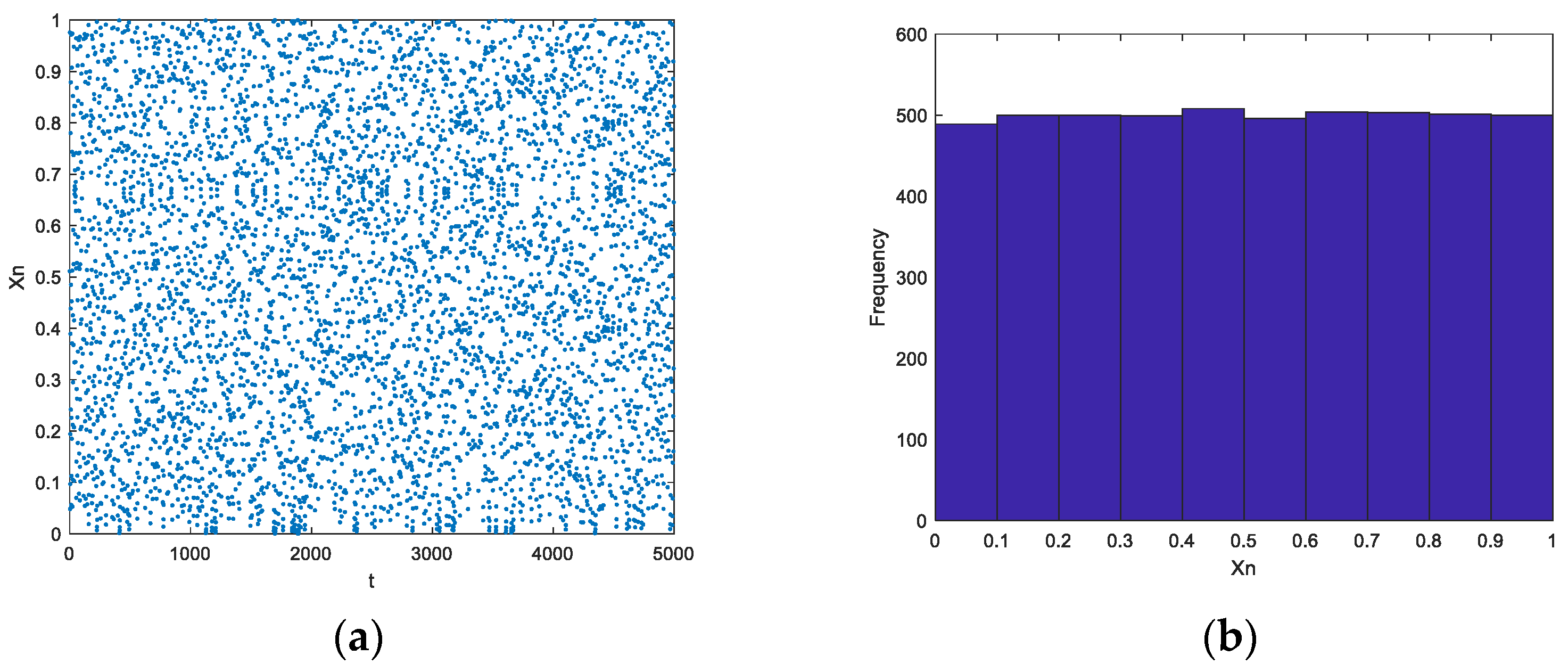
The DBO is a novel swarm intelligence optimization algorithm proposed by Professor Shen Bo’s team in 2022, inspired by the ball rolling, dancing, foraging, stealing, and breeding behavior of dung beetles [10]. Simple and effective, the DBO has been successfully applied to several engineering design problems and outperforms other metaheuristic algorithms in the shelf-life prediction of this paper. However, the DBO still suffers from the problems of an imbalance between global and local search capabilities and the tendency to fall into local optimal solutions [9]. To address these problems, the dung beetle optimizer using Gaussian distribution estimation strategy (GDEDBO) is proposed in this paper based on the original algorithm with the following improvement strategy.

Chaotic Mapping

Chaotic mapping is a method that aims to overcome the problem of heuristic algorithms getting trapped in local optima. It is inspired by the chaotic phenomenon that some systems may have unpredictable variables [16]. By introducing unknown variables into a heuristic algorithm and applying the principle of chaotic phenomena, the algorithm’s accuracy can be improved, and the global search ability can be enhanced [17]. The tent chaotic mapping can generate a uniform chaotic sequence in the 0,1 interval, where x i is the i th particle in the chaotic sequence, as shown in Equation (12):
x i + 1 = 2 x i , 0 x i < 0.5 2 1 x i , 0.5 x i < 1 .
Since the chaotic sequences generated by the chaos operator during the iterative process are periodic and more likely to fall into unknown periodic points, the random variable r a n d function can be added to stabilize them. The t e n t operator requires the ability to handle large amounts of data via Bernoulli transformation and yields Equation (13), where r a n d 0,1 is a random number in the 0,1 interval of random numbers:
x i + 1 = 2 x i + r a n d 0,1 , 0 x i < 0.5 2 1 x i + r a n d 0,1 , 0.5 x i < 1 .
To generate a more uniform initialization of the population than the original DBO algorithm, which used a random initial population, this paper applied tent chaos mapping. This method produces a relatively uniform distribution of the system that can enhance the diversity of the population and improve the initial solution of the algorithm. Figure 1 shows the distribution of the initialized populations using tent chaos mapping and the random method.

Elite Pool Strategy

The elite pool strategy is a commonly used improvement method for swarm intelligence optimization algorithms that aims to preserve a certain number of the current optimal solutions after each iteration and replace some worse solutions with them in the next iteration, thus retaining excellent solutions and accelerating convergence. This paper defines the rolling dung beetle as the leader and introduces the elite pool strategy into its position update formula to enhance the diversity of the leader. The rolling dung beetle is the first to start searching, and its position update mode is affected by the global worst position (the sun) and obstacles. To avoid local optima and enhance population diversity, this paper proposes an elite pool strategy by referring to the hierarchy of the GWO algorithm, in which the top 3 currently optimal individuals and the weighted average position of the leader population are stored, as shown in Figure 2. The 3 optimum individuals can better help the rolling dung beetle determine its rolling direction, while the weighted average position represents the evolutionary trend of the whole dominant population, which is beneficial for algorithm exploration. The leader randomly selects an individual from the elite pool as the rolling direction when updating its position, which to some extent avoids the deficiency of being trapped in a local optimum due to having only one rolling direction. The elite pool strategy is described as follows:
X Elite t = X best1 t , X best2 t , X best3 t , X mean t
X mean t = i = 1 N / 2 w i × X t i
w i = ln N / 2 + 0.5 ln i i = 1 N / 2 ln N / 2 + 0.5 ln i
where X best1 t , X best2 t , and X best3 t are the top three individuals with the best fitness value of the current population, respectively; X mean t denotes the weighted average position of the rolling dung beetles; N is the population size; X i t is the position of the i th rolling dung beetle in generation t ; and w i denotes the weighting coefficients among the rolling dung beetles in descending order of fitness value.
The adjusted formula for updating the position of the rolling dung beetle is as follows:
X i t + 1 = X i t α X i t X Elite t X i t X Elite t ,   a c c e s s i b l e   m o d e X i t tan θ X i t X Elite t X i t X Elite t ,   b a r r i e r   m o d e X Elite t X best 1 t , X best 2 t , X best 3 t , X mean t
where X Elite t is a randomly selected individual in the elite pool, α denotes the roll speed coefficient, and θ denotes the roll direction.

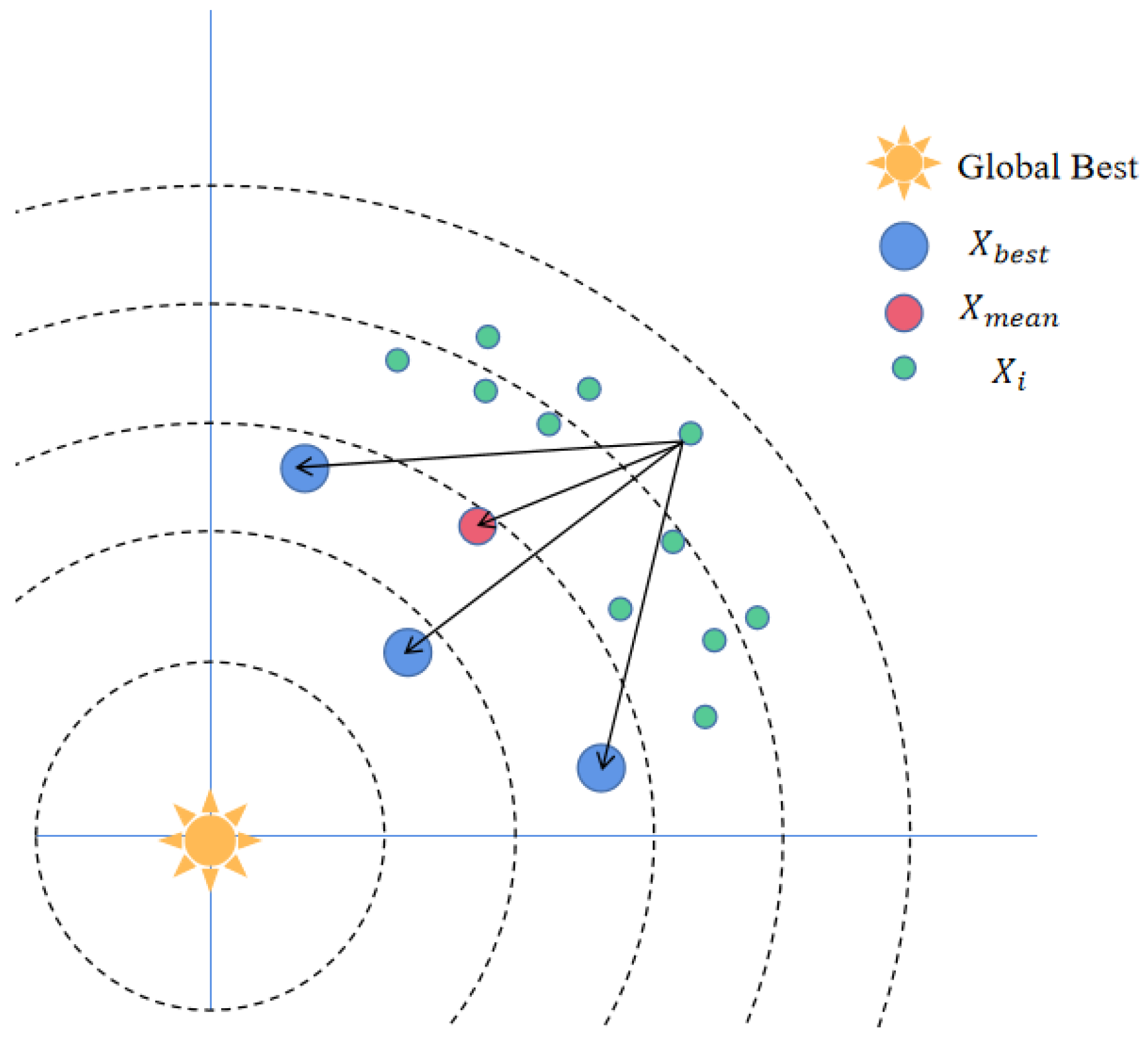
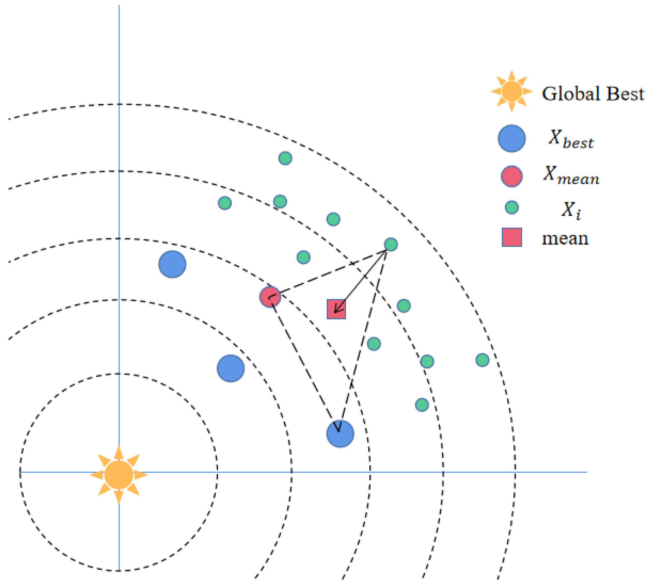
Gaussian Distribution Estimation Strategy

The Gaussian distribution estimation strategy is a position update method based on probability distribution that simulates information exchange and knowledge sharing among population individuals by using the Gaussian distribution function to improve population diversity and exploration. In this paper, spawning dung beetles and small dung beetles are defined as followers. Spawning dung beetles are generated by rolling dung beetles, whose position updates are attracted by the local optimal position (spawning area) to increase search accuracy; small dung beetles are hatched by spawning dung beetles, whose position updates are attracted by the global optimal position (optimal foraging area) to further improve search accuracy. However, the position updates of the spawning dung beetles and the small dung beetles depend only on information about themselves and adjacent individuals, and a lack of communication with other individuals can easily lead to local optimums converging prematurely. To enhance the optimization ability of the algorithm, this paper improves the follower position formula by using the Gaussian distribution estimation strategy. The formula is as follows:
X i t + 1 = mean + y , y N 0 , Cov ,
mean = elite t + X m e a n t + X i t 3
Cov i = 1 N / 2 i = 1 N / 2 X i t X m e a n t × X i t X m e a n t T
where Cov is the weighted covariance matrix of the dominant population. Figure 3 shows that by using the Gaussian distribution estimation strategy to adjust the search direction, the algorithm can effectively balance the global and local search abilities and fully utilize the dominant population information to guide the better evolution of the population, thus enhancing the algorithm’s search performance.
Finally, a superiority mechanism is applied to preserve the dominant individuals and thus ensure the convergence of the IDBO algorithm, with the following position update formula:
X i t + 1 = X i t + 1 ,   f X i t + 1 < f X i t X i t ,   f X i t + 1 > f X i t .

2.4.3. The MRMR-GDEDBO-BPNN Model

The MRMR-GDEDBO-BPNN model proposed in this paper consists of four main components, as follows:
(1)
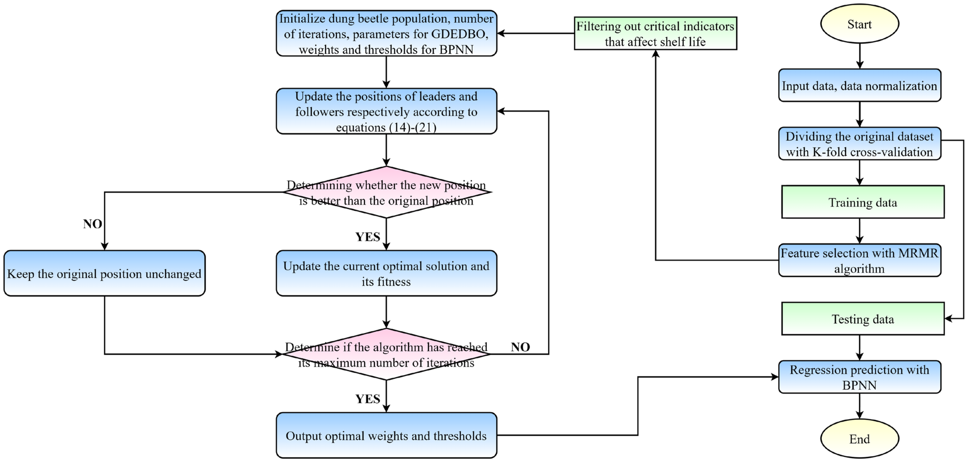
Feature selection: The MRMR algorithm was used to select the key factors for predicting the shelf life of blueberries as input. This algorithm reduced the feature dimensionality by filtering out redundant features that could affect the model prediction accuracy;
(2)
The GDEDBO model: To address the problems of the original DBO, this paper proposes three improvement strategies. First, tent chaotic mapping was introduced to initialize the dung beetle population and increase its diversity. Second, enhancing the diversity of leaders by introducing an elite pool strategy to improve the exploration performance of the algorithm; and third, using the Gaussian distribution estimation (GDE) strategy to use dominant population information to adjust the search direction to guide the population to better evolution;
(3)
The GDEDBO-BPNN model: The GDEDBO-BPNN used the GDEDBO to optimize the parameter weights w and thresholds b of the BPNN and updated the w and b of the BPNN by continuously updating the positions of the dung beetles until the global best position, i.e., the optimal solution, was found;
(4)
Forecasting model and evaluation of results: The MRMR-GDEDBO-BPNN model predicted the shelf life of blueberries, using the physicochemical and quality indicators selected by the MRMR algorithm as input parameters and selecting different evaluation indicators to evaluate the prediction results. Figure 4 shows the flow chart of the MRMR-GDEDBO-BPNN model.

3. Experimental Simulation and Analysis

In order to fully verify the superior performance of the GDEDBO algorithm, this paper selects 14 standard test functions from the IEEE CEC2017 single-objective test function set to test the performance of the algorithm. As shown in Table 3, F1–F8 belong to unimodal test functions, which are used to check the convergence accuracy of the algorithm; F9–F14 belong to multimodal test functions, which are used to test the ability of the algorithm to jump out of the local optimum. The hybrid firefly and particle swarm optimization (HFPSO) [18], the gray wolf optimization algorithm with a hybrid Gaussian distribution estimation strategy (GEDGWO) [19], the Harris Hawk optimization algorithm (HHO) [20], and the original DBO algorithm were also selected as comparison algorithms, with their parameter settings referring to the original literature, as shown in Table 4. HFPSO is an improved particle swarm algorithm with a hybrid firefly algorithm. GEDGWO is a variant of the GWO algorithm incorporating a distribution estimation algorithm. Both of these improved algorithms have demonstrated good performance in their respective literature, while HHO and DBO are the latest proposed swarm intelligence optimization algorithms that have performed well in recent years and have been applied in different disciplines and engineering fields. Therefore, a comparison using these algorithms can improve the validity of the improvement strategies proposed in this paper. To ensure fairness, the number of populations N = 50, dimension D = 30, and the maximum number of iterations were set uniformly at 500. Each algorithm was run 50 times independently, and the optimal value, mean, and standard deviation of the fitness were recorded to evaluate the exploration performance, convergence accuracy, and stability of the algorithms. The experiments were implemented using MATLAB 2022b on a Windows 11, 64 bit system with an Intel® Core™ i7-11700 2.5 GHz, 16 GB RAM computer. The experimental results are shown in Table 5.

3.1. Development and Exploration Capacity Assessment

As can be seen from Table 5, for the unimodal test functions F1 to F8, GDEDBO achieved better solutions on six functions except F5 and F6, indicating that the enhancement strategy can effectively improve the development of the algorithm. GEDGWO ranked first on F5. For the multimodal test functions F9 to F14, GDEDBO ranked first on four functions except F11 and F13, and GEDGWO performed better on F11. For F9, although all the algorithms converge to the theoretical optimum, only DBO and GDEDBO have a mean and standard deviation of 0, indicating that their stability and exploration of the multimodal functions are better than those of the other compared algorithms. It proves that the improvement strategy proposed in this paper can enhance the exploitation and exploration capabilities of the algorithm.

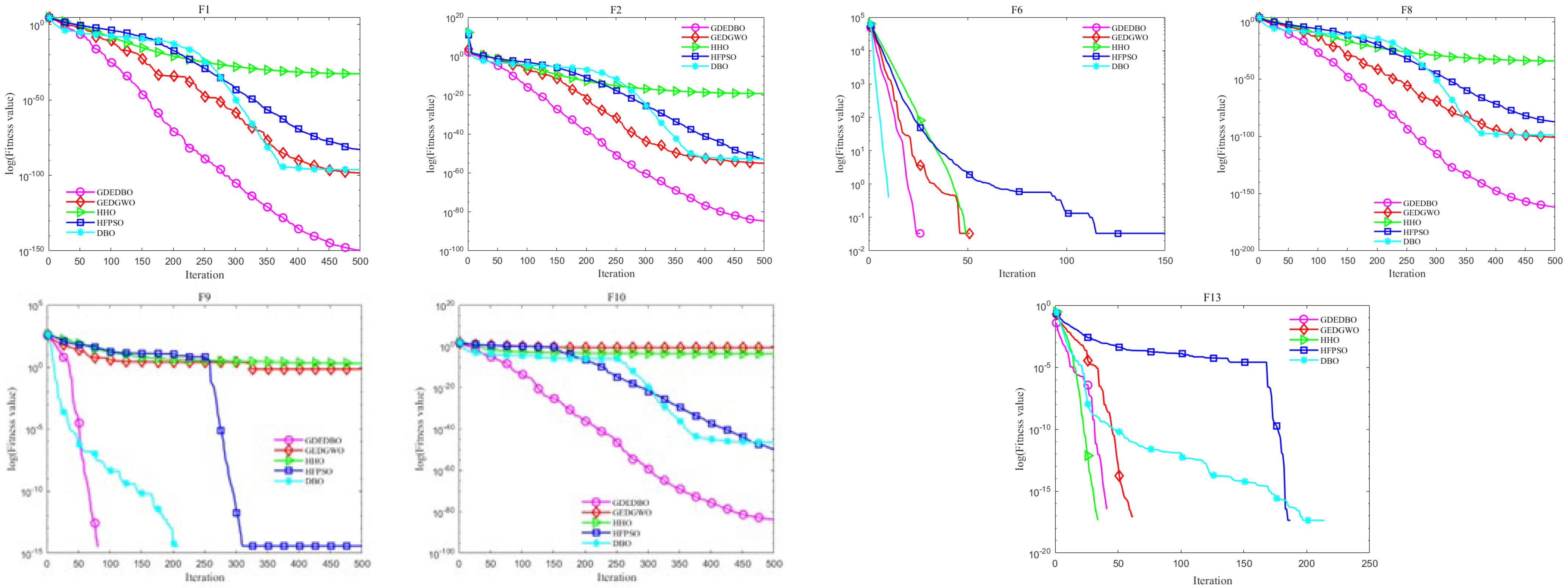
3.2. Convergence Curve Analysis

In order to reflect more intuitively the convergence speed of each algorithm and the ability to jump out of the local optimum, the convergence curves of some of the tested functions are shown in Figure 5. As can be seen from Figure 5, GDEDBO has faster convergence speed and convergence accuracy on five functions except F6 and F13. DBO ranks first on F6 and has a faster convergence speed than GDEDBO, which may be due to the elite pooling strategy. GDEDBO ranks second on F13, which proves that the improvement strategy proposed in this paper can effectively improve the convergence performance of the algorithm.

3.3. Wilcoxon Rank Sum Test

The robustness of the algorithms was evaluated by applying the Wilcoxon rank sum test to compare the overall results of the algorithms. The Wilcoxon rank sum test was conducted at the 5% significance level, and a p -value less than 5% indicated a significant difference between the two compared algorithms, while a p -value greater than or equal to 5% indicated no significant difference or similar performance in finding the best solution. In this study, five algorithms were used as samples, and each algorithm was run 50 times independently with a population size of N = 50 and a dimension of D = 30 on 14 standard test functions. The results obtained by the GDEDBO were compared with those obtained by the four other algorithms using the Wilcoxon rank sum test. The p -values from the Wilcoxon rank sum test are presented in Table 6. N/A means not applicable, as both merit search results are 0 and there is no data to compare, indicating similar performance. As shown in Table 6, most of the p -values are less than 5%, suggesting that the GDEDBO model has a significant difference from the other comparison algorithms.
The results of the benchmark function test, the convergence curves of some of the tested functions, and the Wilcoxon rank sum test results of each algorithm were combined to assess the performance of the GDEDBO. It was found that the GDEDBO had significantly enhanced local and global capabilities and outperformed comparative optimization algorithms such as the original DBO and HHO, showing better exploration performance, convergence accuracy, and stability.

4. Model Parameter Settings and Evaluation Criteria

4.1. Model Parameter Settings

4.1.1. The Baseline Model

The performance of the MRMR-GDEDBO-BPNN model proposed here was verified by comparing it with MLR, SVR, ANN, BPNN, MRMR-BPNN, DBO-BPNN, MRMR-DBO-BPNN, GDEDBO-BPNN, and MRMR-GDEDBO-BPNN as the benchmark models. Grid search was used to optimize the parameters of the benchmark models for improved training speed and accuracy. Table 7 and Table 8 show the optimal parameter combinations for the SVR and ANN models and for the BPNN model, respectively.

4.1.2. The BPNN Model

Choice of Network Functions

BPNNs commonly employ functions such as activation functions, training functions, learning functions, etc.
The activation function is a key component of a neural network that determines how the neurons generate outputs from the inputs. Activation functions enable neural networks to model nonlinearly, allowing them to approximate complex data and functions [21]. The activation functions frequently used in BPNNs are the logistic function LOGSIG, the hyperbolic tangent function TANSIG, the linear function PURELIN, and the rectified linear unit POSLIN. LOGSIG and TANSIG are often applied as activation functions for the input layer, while PURELIN is often applied as the activation function for the output layer. This paper determines the activation function that minimizes the model error by trial and error and presents the results in Table 8. It shows that the activation function combination that minimizes the error of the MRMR-GDEDBO-BPNN model at three temperatures, 0, 4, and 25 °C, is LOGSIG-PURELIN.
The training functions of BPNN are functions used to adjust the network parameters, usually based on the gradient descent method or its variants, aiming to minimize the network error. Commonly used training functions include trainlm, trainrp, trainscg, trainbfg, and traingdx. Among them, trainlm is an algorithm that combines gradient descent and Newton’s method, which has the advantages of fast convergence and high accuracy, so this paper uses trainlm as the training function.
The common learning functions of BPNN include learngd (gradient descent method) and learngdm (gradient descent method with momentum). The learngd function only adjusts the weights and bias according to the gradient direction and learning rate, which are slow to converge and prone to falling into local optima. The learngdm function increases the momentum constant to effectively overcome the drawbacks of the gradient descent method, so this paper uses learngdm as the learning function, and its formula is shown in (22):
Δ W = α Δ W p r e v 1 α η E W ,
where Δ W denotes the amount of change in weight or bias; α denotes the momentum constant, between 0 and 1; Δ W p r e v denotes the amount of change in the previous weight or bias; and η denotes the learning rate; E W denotes the direction of the gradient.

Selection of Topologies

The topology of the BPNN model is formed by the number of neurons in each layer and the connections between two adjacent layers. The topology affects the complexity and expressiveness of the neural network, which in turn affects its performance and convergence speed [22]. Therefore, selecting a suitable topology is a critical step in neural network design. The optimal number of neurons in the hidden layer should avoid underfitting and overfitting. Underfitting occurs when the network has insufficient neurons in the hidden layer to capture the complex features of the data. Overfitting or gradient vanishing occurs when the network has excessive neurons in the hidden layer that fit too closely to the training data [23]. The number of neurons in the hidden layer is not fixed but varies according to the complexity of the problem and the size of the data. Choosing an appropriate number of neurons in the hidden layer is essential for improving the generalization and prediction abilities of the model.
An empirical formula (Equation (23)) was proposed to estimate the number of neurons in the hidden layer, which ranged from 4 to 12. The optimal number of neurons for different models with the minimum error was obtained by grid search and manual parameter tuning, as shown in Table 8. Table 8 shows that the MRMR-GDEDBO-BPNN model had the lowest error with 5 neurons in the hidden layer (single layer) at all three temperatures of 0, 4, and 25 °C.
N h = N i + N o + α , α   ϵ   1,10 ,
where N h , + + N i , and N o represent the number of neurons in the hidden layer, input layer, and output layer, respectively, and α is a modulation constant between 1 and 10.
The hidden layer of a neural network allows it to handle non-linearly separable data, which cannot be represented by a neural network without hidden layers [22]. The number of hidden layers influences the representation and adaptation of a neural network. More hidden layers generally reduce error but also increase complexity, training difficulty, and the risk of overfitting. This paper used double hidden layer and single hidden layer neural network models for 23 input variables without feature selection and 7 input variables after MRMR filtering, respectively. Different combinations of activation functions were also tested to determine the optimal network topology.
Table 8 shows that the best topology for the GDEDBO-BPNN model with the lowest error without feature selection was 23–8−8–1 at 0, 4, and 25 °C. After MRMR selection, the best topology for the MRMR-GDEDBO-BPNN model with the lowest error at all three temperatures was 7−5–1 (as shown in Figure 6).

Network Training

The network training parameters included an upper limit of 100 iterations, a performance target error of 0.0001, a population size of 50, a learning rate of 0.01, and a momentum constant with a default value of 0.9.

4.2. Model Evaluation

4.2.1. K-Fold Cross-Validation

K-fold cross-validation is a widely used technique for model evaluation and parameter tuning. It can reduce the variability of data splitting and enhance the generalization ability of the model [24]. This paper used a 10-fold cross-validation method to build the model, i.e., the data was divided into 10 subsets. The cross-validation was repeated in 10 rounds. In each round, the data were randomly split into a training set and a test set. The model was trained on the training set and validated on the test set. The model performance metrics (e.g., MSE values) were averaged over 10 rounds as an estimate of the model’s prediction accuracy. The optimal results are shown in Table 8, where the neuron configuration that minimized the model error at 0 °C for the BPNN model, for example, was a two-layer hidden layer of (6,7).

4.2.2. Evaluation Indicators

Statistical error is widely used to assess the predictive performance of a model. Common regression evaluation metrics include mean absolute error (MAE), mean squared error (MSE), mean absolute percentage error (MAPE), and coefficient of determination ( R 2 ). MAE indicates the difference between the optimal value of the algorithm and the theoretical optimal value and reflects the exploration capability and convergence accuracy of the algorithm. MAPE measures the relative error between predicted and true values and is expressed as a percentage. It is useful for comparing models with data at different scales. R 2 measures how well the model fits the data; as it approaches 1, the better the model fits, and conversely, as it approaches 0, the worse the fit. The formula is as follows:
M A E = 1 N i = 1 N Y i Z i ,
M S E = 1 N i = 1 N Y i Z i 2 ,
M A P E = 1 N i = 1 N Y i Z i Y i × 100 % ,
R 2 = 1 i = 1 n Y i Z i 2 i = 1 n Y i Y i ¯ 2 ,
where Y i and Z i denote the true and predicted values, respectively.

5. Results

The critical factors affecting the shelf life of blueberries filtered by the MRMR algorithm in this paper were: total color difference, weight loss, hardness, decay rate, soluble solids content, pH, and sensory evaluation score. Figure 7, Figure 8, Figure 9, Figure 10 and Figure 11 show the trends of these seven quality indicators with storage time at different storage temperatures.

5.1. Trends in Quality Indicators of Blueberries at Different Storage Temperatures

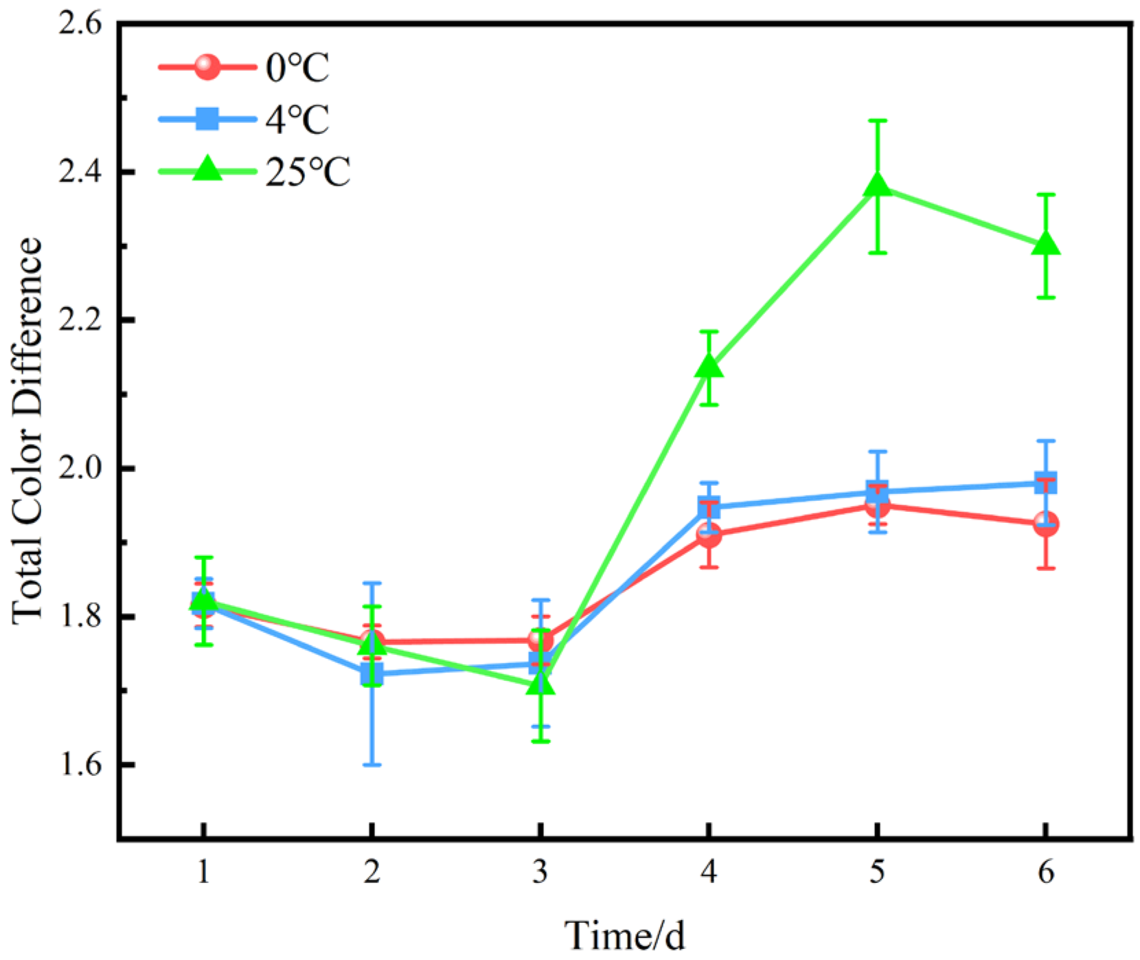
5.1.1. Total Color Difference

Anthocyanins are the main pigments that determine the color of blueberry fruit, which is important for both aesthetic and nutritional value. However, anthocyanins are susceptible to degradation during storage due to various factors, such as condensation with proanthocyanidins, enzymatic oxidation by peroxidases and polyphenol oxidases, and binding to macromolecules (e.g., proteins and cell wall polysaccharides) to form precipitates [25]. Anthocyanin degradation can result in a color change from blue-purple to red, which may reduce consumer acceptance. Therefore, it is of interest to investigate the color characteristics of blueberry fruit stored at different temperatures and to develop effective preservation strategies to retain anthocyanins as much as possible.
Total color difference ( Δ E ) is a common colorimetric parameter to describe the color variation of fruits. A Δ E value less than 1.0 indicates an insignificant color difference; a value less than 2.0 indicates a detectable color difference by trained observers; and a value above 3.5 indicates a noticeable color difference by average consumers [26]. As shown in Figure 7, Δ E increased after 3 d of storage at 0, 4, and 25 °C, with a similar trend at 0 °C and 4 °C and a larger increase at 25 °C. This may be attributed to the higher anthocyanin retention at low temperature storage [27]. However, this color change was not statistically significant and was not easily perceived by the average consumer (maximum Δ E < 2.5), as shown in Figure 7.

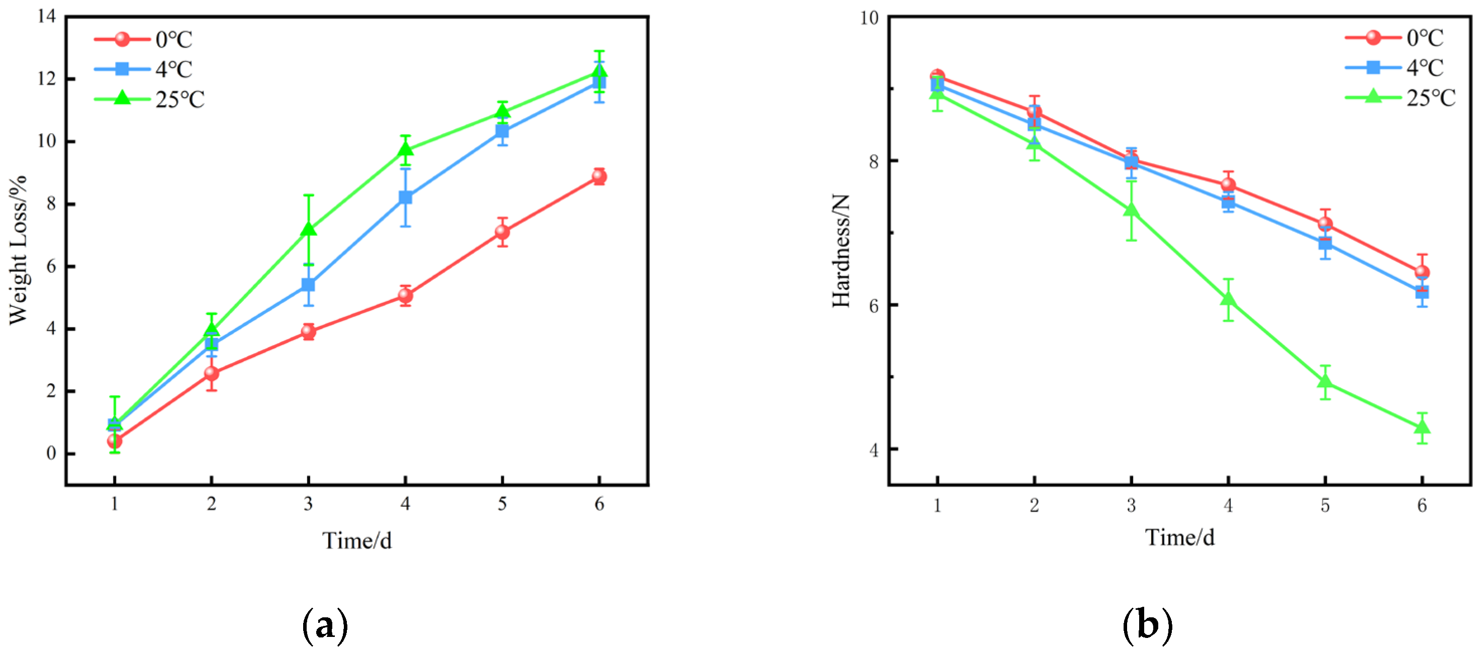
5.1.2. Weight Loss and Hardness

Figure 8 shows the effects of storage time and temperature on weight loss and fruit hardness in blueberries. During storage, blueberries undergo respiration and transpiration processes that result in moisture loss, macromolecule degradation, mass reduction, weight loss increase, and fruit hardness decrease. The hardness of blueberries stored at 0, 4, and 25 °C decreased by 32.68%, 34.53%, and 55.36%, respectively, after 6 days of storage, indicating that lower storage temperatures could better preserve the fruit’s firmness and that 0 °C was more effective than 4 °C in delaying fruit softening.

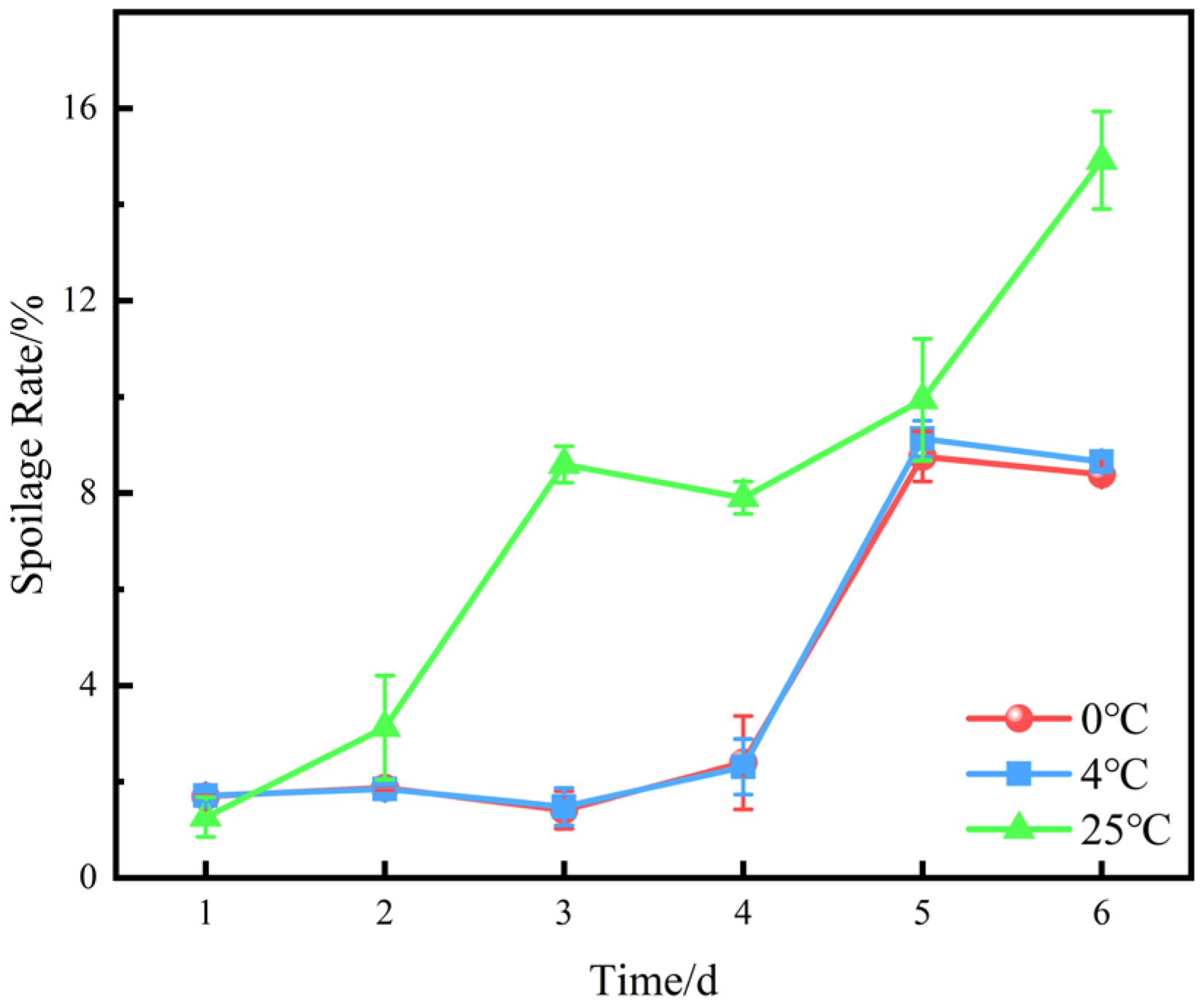
5.1.3. Spoilage Rate

Figure 9 shows the spoilage rates of blueberries stored at 0 °C, 4 °C, and 25 °C. At 0 °C and 4 °C, the spoilage rates were similar and remained stable for the first 3 days, followed by a sharp increase after day 4. At 25 °C, the spoilage rate increased rapidly from day 2 and reached a plateau for the last 3 days. This could be attributed to the effects of temperature and confined space on microbial growth and metabolic activity. The spoilage rates at day 6 were 7.66%, 7.92%, and 16.44% for 0 °C, 4 °C, and 25 °C, respectively. These results indicate that low temperatures can delay spoilage and extend the shelf life of blueberries, and that 0 °C is more effective than 4 °C in inhibiting spoilage.

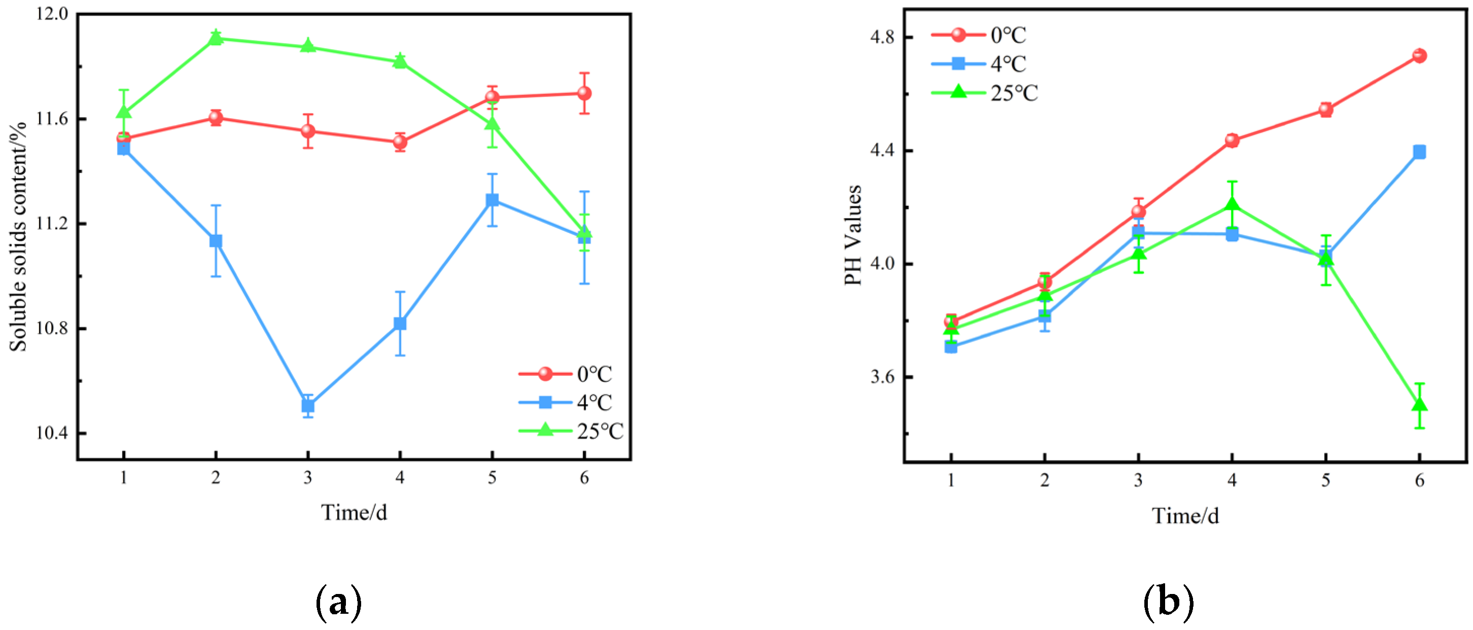
5.1.4. Soluble Solids Content and pH Values

Figure 10 shows that the SSC of blueberries increased significantly after 2 days of storage at 0 °C and 4 °C. This could be attributed to the degradation of polysaccharides and the conversion of organic acids, which enhanced the sweetness of the fruit. At 25 °C, the SSC increased rapidly after 3 days of storage, which might reflect the different ripening stages of the fruit at harvest [28]. Fluctuations in SSC and pH values were observed at all storage temperatures, especially at 25 °C. These fluctuations could be related to changes in fruit metabolism induced by respiration, which is more intense at higher temperatures. These results indicate that low-temperature storage can extend the shelf life of blueberries by reducing their respiration rate.

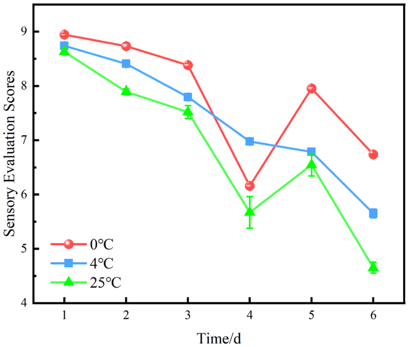
5.1.5. Sensory Evaluation Scores

Sensory evaluation is a subjective measure of human perception of changes in blueberry quality. Figure 11 shows that the overall sensory score of blueberries was the lowest at 25 °C. This was consistent with Table 2, which showed that blueberries stored at 25 °C for 6 days had a dull and lusterless appearance, severe quality loss, and a 50% decay area. The sensory scores of blueberries were higher at 0 °C and 4 °C, with the highest score at 0 °C.

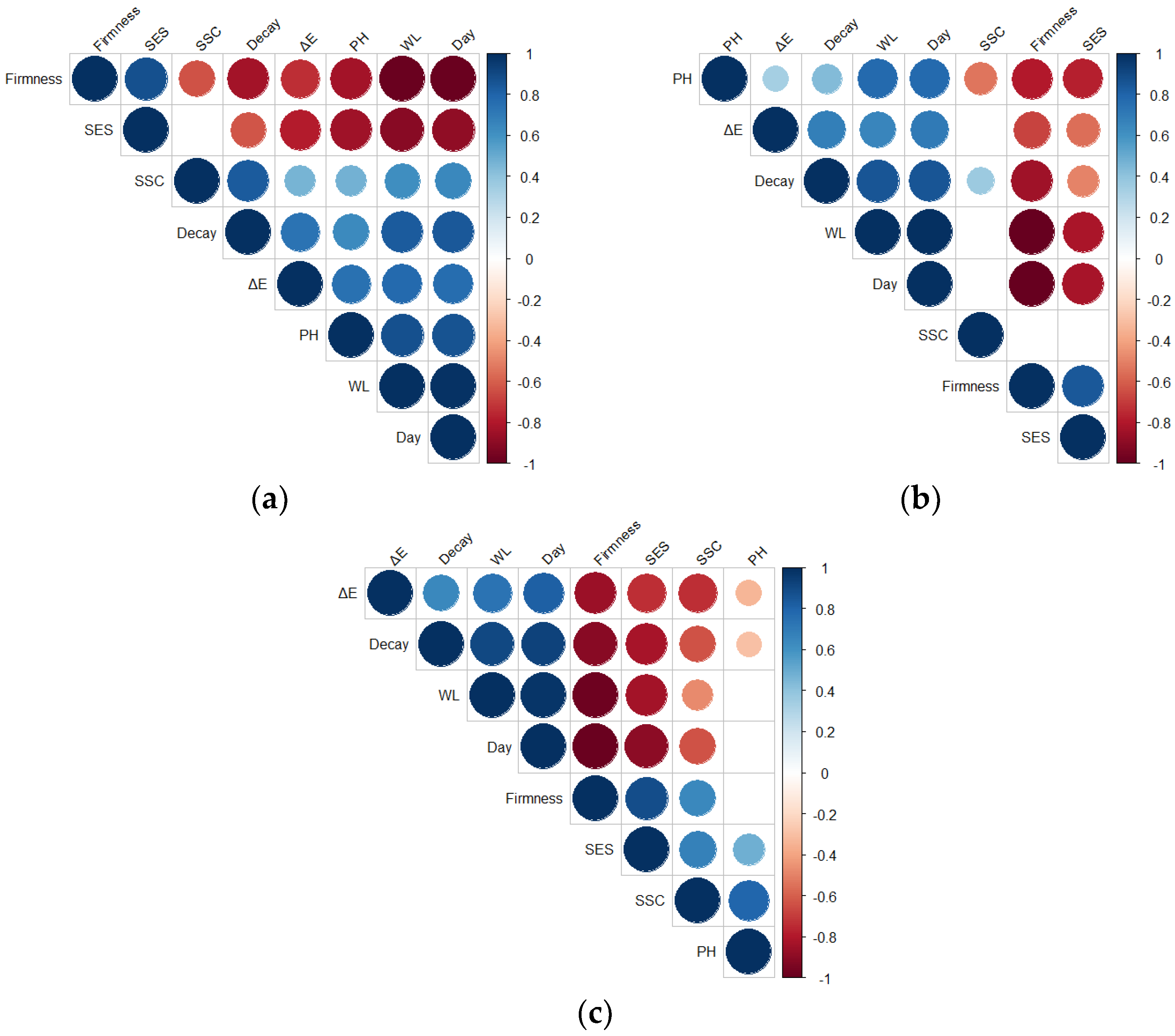
5.2. Pearson’s Correlation Analysis

The quality attributes of blueberries changed significantly during storage, and these changes were correlated with each other and affected the shelf life of the fruit. Pearson correlation analysis was performed on the seven key factors selected by the MRMR algorithm and the storage time, as shown in Figure 12 (sorted by hclust hierarchical clustering order). Figure 12 shows that there was no significant correlation ( p < 0.01 ) between soluble solids content and other factors at 4 °C or between pH value and other factors at 25 °C. At all storage temperatures, weight loss and firmness had the highest correlation with shelf life. The correlation analysis results indicate that the shelf-life prediction model based on quality indicators and sensory evaluation scores of blueberries is reliable.

5.3. Model Performance Comparison Analysis

The prediction performance of each model on the test set is shown in Table 9, from which it can be seen that (taking 0 °C as an example):
(1)
Compared with the benchmark model, the MRMR-GDEDBO-BPNN model proposed in this paper performed the best, with its MAE, MSE, MAPE, and R2 of 0.0304, 0.0014, 1.1379%, and 0.9995, respectively, significantly outperforming the other models;
(2)
Compared with the MLR, ANN, and SVR models, the BPNN model reduced the MAE, MSE, and MAPE values by 56.13–60.02%, 99.54–99.60%, and 35.68–51.71%, respectively. Compared with MRMR-MLR, MRMR-ANN, and MRMR-SVR models, the MRMR-BPNN model reduced the MAE, MSE, and MAPE values by 74.83–78.25%, 99.62–99.69%, and 39.47–43.38%, respectively. These results indicate that the BPNN model had better prediction performance than other models, regardless of feature selection, indicating that the BPNN model has a stronger fitting and generalization ability for the dataset in this paper. The possible reasons are as follows: The MLR model may fail to capture the nonlinear features and complex relationships of the data, leading to large prediction errors [29]. The BPNN model can fit the data more accurately than the ANN model because the BPNN model uses the structure of a multilayer perceptron to learn the high-order features and complex relationships of the data, while the ANN model only uses the structure of a single-layer perceptron. The SVR model is a regression model based on support vector machines, which seeks the optimal hyperplane by maximizing the margin, but the data may not be linearly separable in reality, and the SVR model may not capture the true pattern of the data, resulting in large prediction errors [30];
(3)
Compared with the conventional BPNN model, the DBO-BPNN model decreased the MAE and MAPE values by 10.88% and 29.81%, respectively, and increased the R2 value by 1.09%. This indicates that optimizing the weights and thresholds of BPNN with DBO can significantly improve the prediction performance of the neural network. Compared with MRMR-BPNN, the MAE, MSE, and MAPE values of the MRMR-GDEDBO-BPNN model decreased by 74.11%, 26.32%, and 88.40%, respectively, and increased the R2 value by 2.25%, further demonstrating the importance of optimizing the weights and thresholds of BPNN;
(4)
Compared with DBO-BPNN, the GDEDBO-BPNN model decreased the MAE, MSE, and MAPE values by 18.68%, 35.14%, and 21.25%, respectively, indicating that the prediction results of the GDEDBO-BPNN model were closer to the actual values and verifying the effectiveness of the improved strategy proposed in this study;
(5)
Compared with MLR, ANN, SVR, and BPNN, after feature selection, their MAE, MSE, and MAPE values decreased by 7.20–49.51%, 4.70–32.14%, and 3.34–20.61%, respectively. Compared with GDEDBO-BPNN, the MAE, MSE, and MAPE values of the MRMR-GDEDBO-BPNN model after feature selection decreased by 81.96%, 96.55%, and 79.72%, respectively, and the R2 value increased by 1.15%. This indicates that feature selection can improve the prediction accuracy of the model by effectively reducing redundant features.
Table 9. Comparison of the performance of different benchmark models for predicting the shelf life of blueberries at different storage temperatures.
Model25 °C4 °C0 °C
MAEMSEMAPER2MAEMSEMAPER2MAEMSEMAPER2
MLR0.60880.735322.3812%0.85880.64520.671721.0512%0.86020.58160.708121.0245%0.8716
ANN0.58070.642019.2673%0.86070.56500.626317.6226%0.87770.54930.610617.5959%0.8947
SVR0.57380.658918.4095%0.87710.55190.63716.1159%0.89290.53000.615117.3324%0.9087
MRMR-MLR0.56730.650518.8400%0.86890.55850.631716.8693%0.88530.53970.612916.6905%0.9017
MRMR-ANN0.55070.642016.2673%0.88070.50710.603716.2406%0.88510.50270.581916.2139%0.8895
MRMR-SVR0.53490.565418.0642%0.89040.50070.531217.3591%0.90130.46650.497015.7850%0.9122
BPNN0.28620.004915.3267%0.95160.22260.003513.9958%0.96300.23250.002810.1526%0.9721
MRMR-BPNN0.19550.008413.9324%0.95740.17980.002612.2877%0.97440.11740.00199.8137%0.9775
DBO-BPNN0.22590.090610.7300%0.96390.20400.06118.4364%0.97970.20720.06267.1264%0.9827
MRMR-DBO-BPNN0.12480.05485.0646%0.97930.11830.04015.0379%0.98370.11580.04013.5118%0.9893
GDEDBO-BPNN0.13130.07376.4364%0.97240.20710.06315.7313%0.98330.16850.04065.6121%0.9881
MRMR-GDEDBO-BPNN0.10130.02533.0083%0.99100.06710.00772.3654%0.99710.03040.00141.1379%0.9995
The network performance and regression analysis graphs of the MRMR-GDEDBO-BPNN configuration after training during storage at 0, 4, and 25 °C are shown in Figure 13a–c, respectively. As shown in Figure 13, the best validation performance at 0 °C and 4 °C was achieved at the 32nd and 17th iterations, respectively, with MSE values very close to 0. At 25 °C, although the number of iterations was less than at 0 °C, the error was also larger, with an MSE value of approximately 0.0004. The regression analysis graphs reflect the fit between the predicted values and the actual values of the data. The R values of all four regression lines were very close to one at all three temperatures, indicating a very good consistency between the actual values and the predicted values, which ensured the good generalization ability of the improved neural network model proposed in this study.
Figure 14a–c show the predicted values of the three neural network models BP, GDEDBO-BP, and MRMR-GDEDBO-BP for the shelf life of blueberries at three storage temperatures of 0, 4, and 25 °C compared with the actual values, respectively (the prediction results are shown in Table 10. As shown in Figure 14, compared with the original BP neural network, the predicted values of the BP neural network model after MRMR feature selection and GDEDBO optimization were closer to the actual values and almost completely coincided with the actual value curve, proving the superiority of the MRMR-GDEDBO-BPNN model proposed in this paper in predicting blueberry shelf life.
As shown in Table 10, the average error and prediction accuracy of the three neural network models, BP, GDEDBO-BP, and MRMR-GDEDBO-BP, at 0, 4, and 25 °C were 5.69% and 94.31%, 2.14% and 97.86%, 0.48% and 99.52%, 8.24% and 91.76%, 3.56% and 96.44%, 1.29% and 98.71%, 10.39% and 89.61%, 7.64% and 92.36%, and 2.96% and 97.04%, respectively.
The comparison of the prediction results of three neural network models shows that:
(1)
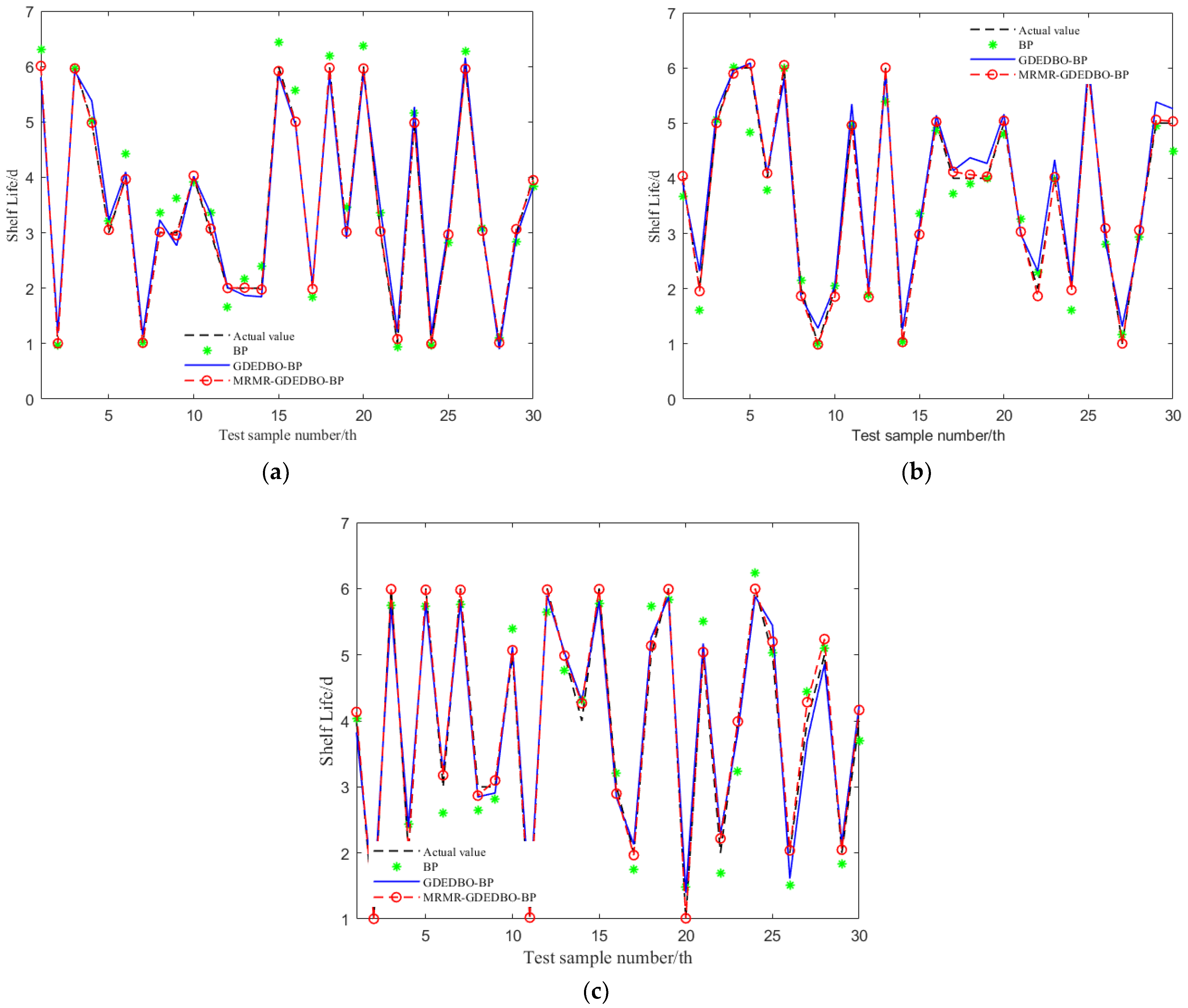
The prediction accuracy of the MRMR-GDEDBO-BP model for blueberry shelf life was the highest, with a prediction error within 3.27%, meeting the needs of shelf-life prediction;
(2)
The prediction error increased with the increase in blueberry storage temperature, which may be due to the fact that the higher the temperature, the stronger the respiration and transpiration of blueberries, resulting in quality decline and shelf-life reduction acceleration, thus increasing the model error. It can be concluded that 0 °C is the best storage temperature for blueberries during their shelf life.

6. Discussion

Shelf life is a complex trait that is greatly influenced by genotype and variety. This study used ‘Liberty’ blueberry as the research object, which was obtained by crossing ‘Brigita’ and ‘Eliot’. Both ‘Brigita’ and ‘Eliot’ are northern highbush blueberry varieties, which have characteristics such as cold resistance, large and sweet fruits, and a long maturation period [31]. ‘Liberty’ blueberries inherited their excellent characteristics and had advantages such as a tall tree body, uniform fruit size, and strong resistance to diseases and pests [25]. These characteristics make ‘Liberty’ blueberries suitable for long-term storage and transportation and provide a good basis for shelf-life prediction. However, the shelf-life prediction problem of ‘Liberty’ blueberries has not been well studied before. Therefore, this paper proposed a novel shelf-life prediction model based on MRMR feature selection and the GDEDBO-BPNN algorithm and achieved high prediction accuracy at three temperatures of 0, 4, and 25 °C. The proposed model outperformed other models or methods reported for different crops in previous studies.
The impact of different input indicators on the model’s prediction accuracy may vary. Figure 12 shows the correlation analysis results of different indicators and shelf-life at 0, 4, and 25 °C. Weight loss and firmness had the highest correlations with shelf life at these temperatures, respectively. Thus, these two indicators could predict the shelf life of blueberries more accurately than others. This agreed with Huang et al., who built blueberry freshness prediction models based on gas information and machine learning algorithms (BP, RBF, SVM, and ELM) at different temperatures and reported that SVM achieved the highest prediction accuracy of 94.01% [8]. However, the proposed model in this paper had a higher prediction accuracy of 96.73%, which might be attributed to the genotype differences that affected the quality change patterns and shelf-life of blueberries and consequently the model’s performance.
Owoyemi et al. applied four models (MLR, SVR, RF, and XGBoost) to predict the shelf-life of ‘Rustenburg’ navel oranges at different temperatures and found that XGBoost performed the best with RMSE and R² of 0.195 and 0.914, respectively, on the whole dataset [30]. Zhang et al. used two methods (PLS and ANN) to establish the shelf-life prediction models of postharvest apples at 4 °C and 20 °C and found that ANN outperformed PLS with the optimal RMSE and R² of 3.51 and 0.991, respectively, under multiple indicators [6]. However, the proposed model in this paper had a higher prediction accuracy and achieved the optimal RMSE and R² of 0.037 and 0.999, respectively, on the test set. The possible reasons for this are as follows:
(1)
Species differences. The quality change patterns and shelf life of fruits are influenced by their species characteristics, such as moisture content, antioxidant capacity, cell wall structure, sugar-acid ratio, etc. Generally speaking, fruits with higher moisture content, stronger antioxidant capacity, more stable cell wall structure, and a moderate sugar-acid ratio have better quality and a longer shelf life. According to previous studies, ‘Liberty’ blueberry is a high-quality variety with high moisture content (about 85%), strong antioxidant capacity (about 13.8 mmol/100 g), stable cell wall structure (about 0.5%), and a moderate sugar-acid ratio (about 15.6) [25]. However, ‘Rustenburg’ navel orange is a low-quality variety with low moisture content (about 60%), weak antioxidant capacity (about 2.4 mmol/100 g), unstable cell wall structure (about 1.2%), and a high sugar-acid ratio (about 25.4) [30];
(2)
Improper feature selection. Owoyemi et al. did not perform feature selection and might have redundant features. Zhang et al. used PLS to select features, but this method only considered the linear correlation between features and responses without considering the redundancy and nonlinearity among features. However, the MRMR algorithm used in this paper could simultaneously consider relevance, redundancy, and nonlinearity among features. Therefore, it obtained higher prediction accuracy;
(3)
Limitations of the models themselves. Owoyemi et al.’s XGBoost model had problems such as sensitivity to noise and outliers, overfitting, tedious hyperparameter tuning, etc., which affected its generalization ability. Zhang et al. used PLS to build the quality change and shelf-life prediction models of apples, but PLS assumed a linear relationship between features and responses, while there might be a nonlinear relationship in reality. They also used ANN to optimize the parameters of the PLS model, but ANN was prone to falling into local optima and was sensitive to parameter selection. However, the BPNN model used in this paper could handle nonlinear and high-dimensional data and used the GDEDBO algorithm to optimize its parameters to avoid falling into local optima and minimize prediction error. Therefore, it obtained more satisfactory prediction results.
Although the MRMR-GDEDBO-BPNN model proposed in this paper showed good predictive performance for the shelf life prediction of blueberries, there are still some aspects that deserve further discussion. For example, feature selection using the MRMR algorithm is independent of the prediction model, and there is no guarantee that the selected features are necessarily optimal in a given prediction model. In future research, attempts can be made to combine the MRMR algorithm with the embedding method to incorporate the prediction model into the feature selection process.

7. Conclusions

To address the problems of complex and multiple influencing factors on blueberry shelf-life prediction, the low training speed of traditional BPNN, and the possible local optimum of the original DBO algorithm, this paper proposes a blueberry shelf-life prediction model based on MRMR-GDEDBO-BPNN. The main conclusions of this paper are as follows:
(1)
Feature selection helps improve the prediction accuracy of shelf-life models;
(2)
Optimizing the weights and thresholds of the BPNN with DBO helps enhance the prediction performance of the neural network;
(3)
To overcome the limitations of the original DBO algorithm, this paper proposes the GDEDBO model. It uses tent chaotic mapping to initialize the population and increase its diversity. It enhances the diversity of leaders by introducing an elite pool strategy to improve the exploration performance of the algorithm. Moreover, it adjusts the search direction by means of a Gaussian distribution estimation strategy, effectively coordinating the algorithm’s global and local search capabilities and strengthening the algorithm’s late-stage optimization search capability. The GDEDBO is evaluated with four meta-heuristic algorithms, including DBO, on 14 benchmark functions. The results show that GDEDBO exhibits good outperformance for both unimodal and multimodal functions, verifying the effectiveness of the improved strategy and being highly competitive with other meta-heuristic algorithms;
(4)
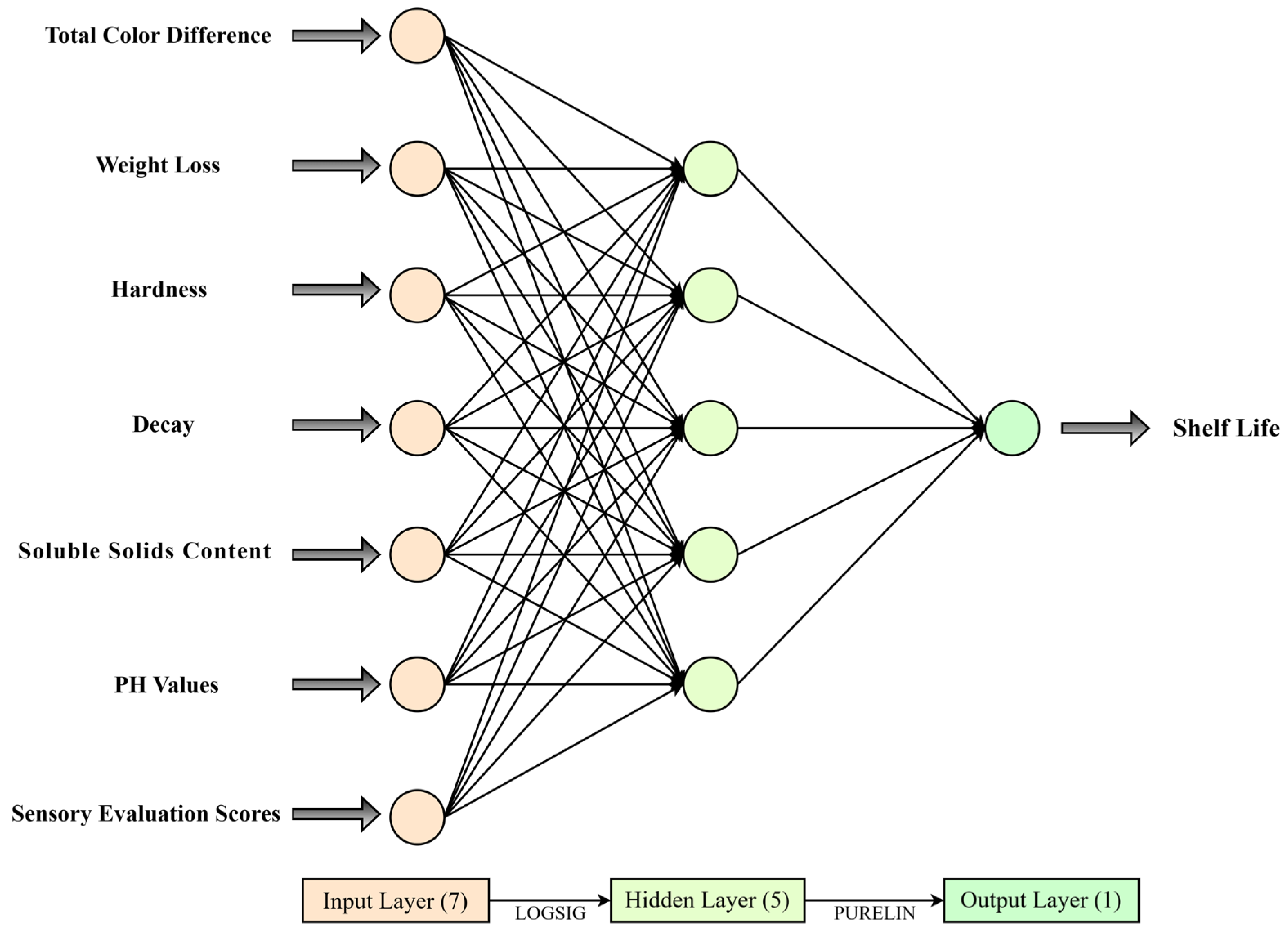
This paper proposed the MRMR-GDEDBO-BPNN model, which uses seven critical factors (hardness, weight loss rate, spoilage rate, total color difference, soluble solids content, pH values, and sensory evaluation scores) filtered by the MRMR algorithm as input variables to establish shelf-life prediction models at three temperatures of 0 °C, 4 °C, and 25 °C, respectively. The results show that compared with the original BPNN, the values of MAE, MSE, and MAPE of the MRMR-GDEDBO-BPNN model are reduced by 86.92%, 50%, and 88.79%, respectively, and the value of R 2 is increased by 2.82%. This indicates that the BPNN model with feature selection by the MRMR algorithm and optimization by the GDEDBO model significantly improved the shelf-life prediction accuracy;
(5)
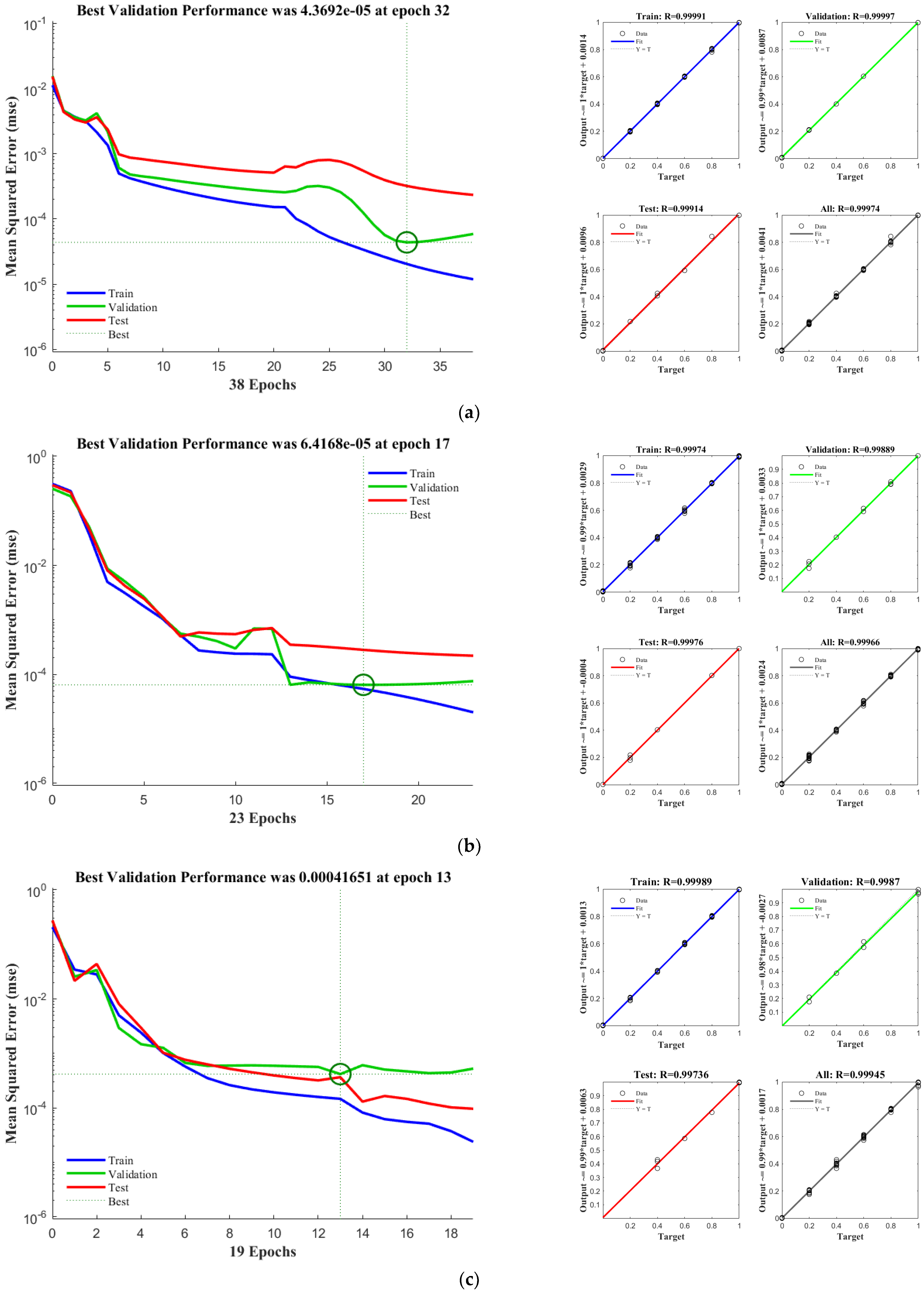
This paper compares the optimal prediction models of shelf life at three storage temperatures, as shown in Table 9. It can be seen from Table 9 that the optimal prediction models at three temperatures are all MRMR-GDEDBO-BPNN models, whose optimal topological structures are all 7–5−1, and the activation function combinations are all LOGSIG-PURELIN. By comparing the prediction accuracy of models at three different temperatures, it can be concluded that the prediction accuracy of shelf-life models at 0 °C and 4 °C is higher than that at 25 °C, and 0 °C is higher than 4 °C. This may be due to the fact that the higher the temperature, the stronger the respiration and transpiration of blueberries, which leads to a faster rate of quality decline and shelf-life shortening, thus increasing the error of the prediction model. It can be concluded that 0 °C is the optimum storage temperature for blueberries during their shelf life;
(6)
This paper compares the shelf life at three storage temperatures with a sensory evaluation score of six as the end point of shelf life. The results are shown in Figure 11. It can be seen from Figure 11 that the shelf lives of this variety of blueberries at 0 °C, 4 °C, and 25 °C are 5.99 days, 5.35 days, and 3.67 days, respectively.
Shelf life is a complex trait that is greatly influenced by genotype and variety. Although the model proposed in this paper achieved high prediction accuracy at three temperatures of 0, 4, and 25 °C, we also recognize that our study has some limitations and shortcomings, such as using only a single Liberty variety of blueberries as the research object, which may cause variety bias by not considering the shelf-life prediction problem of other crops (such as fruits, vegetables, etc.). Therefore, we propose some future directions for further research:
(1)
To train and test the proposed shelf-life prediction model on multiple varieties or genotypes of blueberries, to verify its applicability in evaluating other varieties or genotypes, and to compare its prediction performance with other models or methods;
(2)
To extend the proposed shelf-life prediction model to predict the shelf-life of other crops (such as fruits, vegetables, etc.) and explore their similarities and differences among different crops.

Author Contributions

Conceptualization, R.Z. and Y.Z.; methodology, R.Z. and G.F.; software, R.Z. and S.L.; validation, R.Z. and S.F.; formal analysis, R.Z. and H.W.; investigation, R.Z. and C.Z.; resources, R.Z. and P.D.; data curation, R.Z. and Z.L.; writing—original draft preparation, R.Z.; writing—review and editing, R.Z.; visualization, R.Z.; supervision, R.Z. and S.F.; project administration, R.Z.; funding acquisition, Y.Z. and G.F. All authors have read and agreed to the published version of the manuscript.

Funding

This research was funded by the Fundamental Research Funds for the Central Universities, grant number 2572020BL01, and the Natural Science Foundation of Heilongjiang Province, grant number LH2020C050.

Institutional Review Board Statement

Not applicable.

Data Availability Statement

Not applicable.

Conflicts of Interest

The authors declare no conflict of interest.

References

  1. Zhao, Y.; Zhu, X.; Hou, Y.; Pan, Y.; Shi, L.; Li, X. Effects of harvest maturity stage on postharvest quality of winter jujube (Zizyphus jujuba Mill. cv. Dongzao) fruit during cold storage. Sci. Hortic. 2021, 277, 109778. [Google Scholar] [CrossRef]
  2. Matrose, N.A.; Obikeze, K.; Belay, Z.A.; Caleb, O.J. Plant extracts and other natural compounds as alternatives for post-harvest management of fruit fungal pathogens: A review. Food Biosci. 2021, 41, 100840. [Google Scholar] [CrossRef]
  3. Han, J.W.; Zuo, M.; Zhu, W.Y.; Zuo, J.H.; Lü, E.L.; Yang, X.T. A comprehensive review of cold chain logistics for fresh agricultural products: Current status, challenges, and future trends. Trends Food Sci. Technol. 2021, 109, 536–551. [Google Scholar] [CrossRef]
  4. Mesías, F.; Martín, A.; Hern’andez, A. Consumers’ growing appetite for natural foods: Perceptions towards the use of natural preservatives in fresh fruit. Food Res. Int. 2021, 150, 110749. [Google Scholar] [CrossRef]
  5. Wang, H.; Zheng, Y.; Shi, W. Comparison of Arrhenius model and artificial neuronal network for predicting quality changes of frozen tilapia (Oreochromis niloticus). Food Chem. 2022, 372, 131268. [Google Scholar] [CrossRef]
  6. Zhang, Y.; Zhu, D.; Ren, X. Quality changes and shelf-life prediction model of postharvest apples using partial least squares and artificial neural network analysis. Food Chem. 2022, 394, 133526. [Google Scholar] [CrossRef]
  7. Fan, X.; Jin, Z.; Liu, Y. Effects of super-chilling storage on shelf-life and quality indicators of Coregonus peled based on proteomics analysis. Food Res. Int. 2021, 143, 110229. [Google Scholar] [CrossRef]
  8. Huang, W.; Wang, X.; Zhang, J. Improvement of blueberry freshness prediction based on machine learning and multi-source sensing in the Cold Chain Logistics. Food Control 2023, 145, 109496. [Google Scholar] [CrossRef]
  9. Zhang, R.; Zhu, Y. Predicting the Mechanical Properties of Heat-Treated Woods Using Optimization-Algorithm-Based BPNN. Forests 2023, 14, 935. [Google Scholar] [CrossRef]
  10. Xue, J.; Shen, B. Dung beetle optimizer: A new meta-heuristic algorithm for global optimization. J. Supercomput. 2022, 79, 7305–7336. [Google Scholar] [CrossRef]
  11. Obsie, E.Y.; Qu, H.; Drummond, F. Wild blueberry yield prediction using a combination of computer simulation and machine learning algorithms. Comput. Electron. Agric. 2020, 178, 105778. [Google Scholar] [CrossRef]
  12. Li, Y.; Chu, X.; Fu, Z. Shelf-life prediction model of postharvest table grape using optimized radial basis function (RBF) Neural Network. Br. Food J. 2019, 121, 2919–2936. [Google Scholar] [CrossRef]
  13. Peng, H.; Long, F.; Ding, C. Feature selection based on mutual information: Criteria of max-dependency, max-relevance, and min-redundancy. IEEE Trans. Pattern Anal. Mach. Intell. 2005, 27, 1226–1238. [Google Scholar] [CrossRef] [PubMed]
  14. Rivera, S.; Giongo, L.; Cappai, F. Blueberry firmness—A review of the textural and mechanical properties used in quality evaluations. Postharvest Biol. Technol. 2022, 192, 112016. [Google Scholar] [CrossRef]
  15. Yu, S.; Lan, H.; Li, X. Prediction method of shelf life of damaged Korla fragrant pears. J. Food Process Eng. 2021, 44, e13902. [Google Scholar] [CrossRef]
  16. Lian, S.; Sun, J.; Wang, Z. A block cipher based on a suitable use of the chaotic standard map. Chaos Solitons Fractals 2005, 26, 117–129. [Google Scholar] [CrossRef]
  17. Wu, Q. A self-adaptive embedded chaotic particle swarm optimization for parameters selection of Wv-SVM. Expert Syst. Appl. 2011, 38, 184–192. [Google Scholar] [CrossRef]
  18. Ibrahim, B.A. A hybrid firefly and particle swarm optimization algorithm for computationally expensive numerical problems. Appl. Soft Comput. 2018, 6, 232–249. [Google Scholar]
  19. Wang, X.F.; Zhao, H.; Han, T. A grey wolf optimizer using Gaussian estimation of distribution and its application in the multi-UAV multi-target urban tracking problem. Appl. Soft Comput. 2019, 78, 240–260. [Google Scholar] [CrossRef]
  20. Heidari, A.A.; Mirjalili, S.; Faris, H. Harris hawks optimization: Algorithm and applications. Future Gener. Comput. Syst. 2019, 97, 849–872. [Google Scholar] [CrossRef]
  21. Greff, K.; Srivastava, R.K.; Koutnik, J. LSTM: A Search Space Odyssey. IEEE Trans. Neural Netw. Learn. Syst. 2017, 28, 2222–2232. [Google Scholar] [CrossRef]
  22. Reed, R.; Marks, R.J., II. Neural Smithing: Supervised Learning in Feedforward Artificial Neural Networks; MIT Press: Cambridge, UK, 1999. [Google Scholar]
  23. LeCun, Y.; Bengio, Y.; Hinton, G. Deep learning. Nature 2015, 521, 436–444. [Google Scholar] [CrossRef] [PubMed]
  24. Wong, T.T.; Yeh, P.Y. Reliable Accuracy Estimates from k-Fold Cross Validation. IEEE Trans. Knowl. Data Eng. 2020, 32, 1586–1594. [Google Scholar] [CrossRef]
  25. Dragišić Maksimović, J.; Milivojević, J.; Djekić, I.; Radivojević, D.; Veberič, R.; Mikulič Petkovšek, M. Changes in quality characteristics of fresh blueberries: Combined effect of cultivar and storage conditions. J. Food Compos. Anal. 2022, 111, 104597. [Google Scholar] [CrossRef]
  26. Mokrzycki, W.S.; Tatol, M. Colour difference ΔE—A survey. Mach. Graph. Vis. 2011, 20, 383–412. [Google Scholar]
  27. Singh, B.; Suri, K.; Shevkani, K. Enzymatic Browning of Fruit and Vegetables: A Review. In Enzymes in Food Technology; Springer: Singapore, 2018; pp. 63–78. [Google Scholar] [CrossRef]
  28. Ates, U.; Islam, A.; Ozturk, B. Changes in Quality Traits and Phytochemical Components of Blueberry (Vaccinium Corymbosum Cv. Bluecrop) Fruit in Response to Postharvest Aloe Vera Treatment. Int. J. Fruit Sci. 2022, 22, 303–316. [Google Scholar] [CrossRef]
  29. Ktenioudaki, A.; O’Donnell, C.P.; Emond, J.P. Blueberry Supply Chain: Critical steps impacting fruit quality and application of a boosted regression tree model to predict weight loss. Postharvest Biol. Technol. 2021, 179, 111590. [Google Scholar] [CrossRef]
  30. Owoyemi, A.; Porat, R.; Lichtern, A. Large-scale, high-throughput phenotyping of the postharvest storage performance of ‘rustenburg’ navel oranges and the development of shelf-life prediction models. Foods 2022, 11, 1840. [Google Scholar] [CrossRef]
  31. Piechowiak, T.; Grzelak-Błaszczyk, K.; Sójka, M.; Skóra, B.; Balawejder, M. Quality and antioxidant activity of highbush blueberry fruit coated with starch-based and gelatine-based film enriched with Cinnamon Oil. Food Control 2022, 138, 109015. [Google Scholar] [CrossRef]
Figure 1. Population initialization for the tent chaos mapping: (a) scatter plot and (b) frequency distribution histogram.
Agriculture 13 01784 g001
Figure 2. Elite pool strategy diagram.
Agriculture 13 01784 g002
Figure 3. Gaussian distribution estimation diagram.
Agriculture 13 01784 g003
Figure 4. Flow chart of the MRMR-IDBO-BPNN model.
Agriculture 13 01784 g004
Figure 5. Part of the test function convergence curves.
Agriculture 13 01784 g005
Figure 6. Schematic representation of the optimal topology of the MRMR-GDEDBO-BPNN model for predicting the shelf life of blueberries at different storage temperatures.
Agriculture 13 01784 g006
Figure 7. Variations in total color difference in blueberries at different storage temperatures.
Agriculture 13 01784 g007
Figure 8. Changes in weight loss and hardness of blueberries at different storage temperatures: (a) weight loss and (b) hardness.
Agriculture 13 01784 g008
Figure 9. Variations in spoilage rate of blueberries at different storage temperatures.
Agriculture 13 01784 g009
Figure 10. Changes in soluble solids and pH of blueberries at different storage temperatures: (a) soluble solids content and (b) pH values.
Agriculture 13 01784 g010
Figure 11. Changes in sensory evaluation scores for blueberries at different storage temperatures.
Agriculture 13 01784 g011
Figure 12. Matrix for correlation analysis of quality indicators of blueberries at different storage temperatures ( p < 0.01 ): (a) 0 °C; (b) 4 °C; and (c) 25 °C; the size and color of the circles were positively correlated with the correlation coefficient, i.e., larger circles and darker colors indicated higher correlation coefficients, and vice versa.
Agriculture 13 01784 g012
Figure 13. Network performance plots and regression analysis of the MRMR-IDBO-BPNN model for predicting the shelf life of blueberries at different storage temperatures: (a) 0 °C; (b) 4 °C; and (c) 25 °C.
Agriculture 13 01784 g013
Figure 14. Comparison of predicted and actual values of blueberry shelf life at different storage temperatures by different benchmark models: (a) 0 °C; (b) 4 °C; and (c) 25 °C.
Agriculture 13 01784 g014
Table 1. Attributes of the test personnel.
NumberAgeGenderClass
124FemaleMaster’s degree
235MaleLecturer
321FemaleUndergraduate
430MalePhD
527FemaleAssistant Researcher
632MaleAssociate Professor
718FemaleUndergraduate
858MaleProfessor
923FemaleMaster’s degree
1047MaleFellow
Table 2. Score criteria for the evaluation of blueberry sensory indicators.
Sensory IndicatorsScoring CriteriaScore
Tier 1 IndicatorsSecondary Indicators
AppearanceGlossy rindBright, evenly colored fruit with a glossy surface 9
Bright fruit, largely uniform in color, with a shiny surface7–8
Basically uniform color, increased waxy layer, reduced lustre, slightly glossy surface4–6
Dull surface of the fruit, uneven color, no luster on the surface1–3
Water lossNormal, smooth surface of the fruit, no wrinkling, no elasticity when pressed lightly by hand, no deformation of the fruit9
Slight water loss, no surface wrinkling, elastic when pressed with the hand, slightly wrinkled skin, no deformation of the fruit7–8
Moderate water loss; slight surface wrinkling of the fruit; the wrinkling intensifies when lightly pressed with the hand; the fruit is lightly deformed and inelastic4–6
Heavy water loss, with obvious surface wrinkling of the fruit, which is severely deformed and inelastic when lightly pressed by hand.1–3
WeightlessnessFull fruit with little weight loss9
Slight loss of weight; small area of ruffling or crumpling around the fruit abscission site 7–8
Moderate weight loss; with a medium area of pericarp crinkling or folding around the fruit abscission site5–6
Severe weight loss, with large areas of skin crinkling or folding around the fruit abscission site3–4
Blueberries almost crumpled into dried blueberries, or whole fruit crumpled to resemble mulberries1–2
Degree of decayFruit surface are free of mold spots9
1–3 mold spots on the surface of the fruit7–8
25–50% of the fruit area decayed4–6
Fruit surface decay greater than 50% of the fruit area1–3
FlavorScentHoneyed, richly scented, no bad odor9
Slightly fragrant, slightly light odor, no bad smell7–8
Has an inconspicuous aroma of fruit and no other odor 5–6
No fruit aroma, slight other odor 3–4
No aroma of fruit, bad odor, moldy smell1–2
Sweetness and acidityIntense and sweet9
Sweeter7–8
Moderate5–6
More acidic3–4
Very sour1–2
TasteBrittlenessVery fluffy1–2
Fluffy3–4
Moderate5–6
Crisp7–8
Very crisp9
ChewinessVery poor palatability1–2
Poor palatability3–4
Moderate5–6
Good palatability7–8
Very good palatability9
TightnessVery low1–2
Relatively low3–4
Moderate5–6
High7–8
Very high9
Table 3. Selected standard test functions.
FunctionDimRange f m i n
f 1 x = i = 1 n x i 2 30/50/100[−100,100]0
f 2 x = i = 1 n x i + i = 1 n x i 30/50/100[−10,10]0
f 3 x = i = 1 n j 1 i x j 2 30/50/100[−100,100]0
f 4 x = m a x x i , 1 i n 30/50/100[−100,100]0
f 5 x = i = 1 n 1 100 ( x i + 1 x i 2 ) 2 + ( x i 1 ) 2 30/50/100[−30,30]0
f 6 x = i = 1 n ( x i + 5 ) 2 30/50/100[−100,100]0
f 7 x = x 1 2 + 10 6 i = 2 n x i 2 30/50/100[−100,100]0
f 8 x = i = 1 n x i 2 + i = 1 n 0.5 i x i 2 + i = 1 n 0.5 i x i 4 30/50/100[−5,10]0
f 9 x = i = 1 n x i 2 10 cos 2 π x i + 10 30/50/100[−5.12,5.12]0
f 10 x = i = 1 n x i sin x i + 0.1 x i 30/50/100[−10,10]0
f 11 x = π n { 10 sin π y 1 + i = 1 n 1 y i 1 2 1 + 10 sin 2 π y i + 1 + y n 1 2 } + i = 1 n u x i , 10,100,4 .
w h e r e   y i = 1 + x i + 1 4 , for all i = 1 , , n
u x i , a , k , m = k x i a m                               x i > a       0                                         a < x i < a       k x i a m                       x i < a  
30/50/100[−50,50]0
f 12 x = 0.1 sin 2 3 π x 1 + i = 1 n x i 1 2 1 + sin 2 3 π x i + 1 + x n 1 2 1 + sin 2 2 π x n + i = 1 n u x i , 5,100,4 30/50/100[−50,50]0
f 13 x = 1 n 1 i = 1 n 1 s i × ( sin 50 s i 0.2 + 1 2
s i = x i 2 + x i + 1 2
30/50/100[−100,100]0
f 14 x = sin 2 π y 1 + i = 1 n 1 y i 1 2 1 + 10 sin 2 π y i + 1
+ y n 1 2 1 + sin 2 2 π y n ,
w h e r e   y i = 1 + x i 1 4 ,  for all  i = 1 , , n
30/50/100[−10,10]0
Table 4. Algorithm Parameter Settings.
AlgorithmsParameters Settings
HFPSO C 1 = C 2 = 1.49445 , a = 0.2 , B 0 = 2
γ = 1 , ω i = 0.9 , ω f = 0.5
GEDGWO r 3 0 ,   1 , r 4 0 ,   1 , r 5 0 ,   1
HHO α = 0.01 , β = 1.5
DBO α = β = 0.1 , a = 0.3 , b = 0.5
GDEDBO α = β = 0.1 , a = 0.3 , b = 0.5 , P p e r c e n t = 0.4 t 0.4 0.2 / M ;
Table 5. Results of standard function tests for each algorithm.
FIndexHFPSOGEDGWOHHODBOGDEDBO
F1Best1.67 × 10−952.25 × 10−1817.22 × 10−351.81 × 10−1153.02 × 10−210
Mean2.55 × 10−834.32 × 10−1136.42 × 10−331.31 × 10−999.59 × 10−159
STD1.20 × 10−822.37 × 10−1121.69 × 10−325.51 × 10−995.25 × 10−158
F2Best4.85 × 10−621.16 × 10−853.85 × 10−214.97 × 10−622.26 × 10−109
Mean3.92 × 10−546.14 × 10−616.55 × 10−208.26 × 10−534.20 × 10−83
STD1.89 × 10−532.35 × 10−604.77 × 10−203.59 × 10−522.81 × 10−82
F3Best6.29 × 1035.73 × 10−1492.27 × 10−111.01 × 10−1101.42 × 10−191
Mean2.45 × 1049.90 × 10−459.65 × 10−86.46 × 10−791.22 × 10−115
STD9.33 × 1037.00 × 10−443.94 × 10−74.57 × 10−787.98 × 10−115
F4Best2.99 × 10−64.31 × 10−842.69 × 10−92.57 × 10−571.96 × 10−102
Mean3.70 × 1013.15 × 10−531.88 × 10−87.21 × 10−484.12 × 10−68
STD2.88 × 1012.23 × 10−521.33 × 10−84.23 × 10−472.31 × 10−67
F5Best2.69 × 1011.00 × 10−62.52 × 1012.45 × 1012.44 × 101
Mean2.75 × 1013.01 × 10−32.67 × 1012.52 × 1012.50 × 101
STD4.83 × 10−13.32 × 10−37.85 × 10−17.38 × 10−13.28 × 10−1
F6Best0.00 × 1000.00 × 1000.00 × 1000.00 × 1000.00 × 100
Mean0.00 × 1000.00 × 1000.00 × 1000.00 × 1000.00 × 100
STD0.00 × 1000.00 × 1000.00 × 1000.00 × 1000.00 × 100
F7Best2.01 × 10−881.92 × 10−1555.23 × 10−294.29 × 10−1131.38 × 10−196
Mean9.19 × 10−771.16 × 10−1112.88 × 10−271.03 × 10−933.10 × 10−152
STD4.61 × 10−766.14 × 10−1114.91 × 10−275.39 × 10−931.30 × 10−151
F8Best2.51 × 10−932.02 × 10−1639.38 × 10−372.78 × 10−1183.58 × 10−202
Mean2.98 × 10−832.30 × 10−1107.05 × 10−352.29 × 10−1037.34 × 10−160
STD1.63 × 10−821.26 × 10−1091.25 × 10−346.75 × 10−1033.86 × 10−159
F9Best0.00 × 1000.00 × 1000.00 × 1000.00 × 1000.00 × 100
Mean1.89 × 10−154.61 × 10−13.15 × 1000.00 × 1000.00 × 100
STD1.04 × 10−142.19 × 1004.36 × 1000.00 × 1000.00 × 100
F10Best1.60 × 10−601.08 × 10−803.31 × 10−201.02 × 10−618.18 × 10−112
Mean8.12 × 10−11.48 × 10−13.65 × 10−21.36 × 10−466.70 × 10−85
STD4.45 × 1008.11 × 10−11.97 × 10−17.47 × 10−462.51 × 10−84
F11Best1.02 × 10−38.84 × 10−96.30 × 10−12.45 × 10−112.87 × 10⁻⁶
Mean1.38 × 10−22.60 × 10−63.25 × 10−23.54 × 10−42.27 × 10−5
STD2.42 × 10−22.49 × 10−62.23 × 10−21.40 × 10−33.04 × 10−5
F12Best2.67 × 10−25.18 × 10−109.78 × 10−21.87 × 10−52.84 × 10⁻⁷
Mean2.30 × 10−11.03 × 10−13.90 × 10−11.33 × 10−23.52 × 10−5
STD1.71 × 10−17.80 × 10−22.10 × 10−13.04 × 10−23.61 × 10−5
F13Best0.00 × 1000.00 × 1000.00 × 1000.00 × 1000.00 × 100
Mean1.83 × 10−50.00 × 1000.00 × 1000.00 × 1000.00 × 100
STD7.91 × 10−50.00 × 1000.00 × 1000.00 × 1000.00 × 100
F14Best5.81 × 10−24.27 × 10−95.43 × 10−11.60 × 10−42.03 × 10−8
Mean4.71 × 10−11.19 × 10−11.03 × 1001.04 × 10−25.43 × 10⁻⁵
STD4.66 × 10−11.14 × 10−12.56 × 10−12.72 × 10−26.87 × 10−5
Table 6. p -values of the Wilcoxon rank sum test.
FunctionsHFPSOGEDGWOHHODBO
F17.07 × 10−187.07 × 10−187.07 × 10−189.54 × 10⁻¹⁸
F27.07 × 10−181.08 × 10−177.07 × 10−187.07 × 10⁻¹⁸
F37.07 × 10−181.99 × 10−127.07 × 10−187.07 × 10⁻¹⁸
F47.07 × 10−181.32 × 10−147.07 × 10−187.07 × 10⁻¹⁸
F53.02 × 10−113.01 × 10−113.01 × 10−113.01 × 10⁻¹¹
F6N/AN/AN/AN/A
F73.01 × 10−113.69 × 10−113.02 × 10−113.02 × 10⁻¹¹
F83.01 × 10−111.33 × 10−103.02 × 10−113.02 × 10⁻¹¹
F93.34 × 10−18.15 × 10−21.84 × 10−10N/A
F103.02 × 10−113.02 × 10−113.02 × 10−113.02 × 10⁻¹¹
F113.02 × 10−118.48 × 10−93.02 × 10−111.69 × 10⁻⁹
F121.96 × 10−108.66 × 10−54.08 × 10−118.89 × 10⁻¹⁰
F131.61 × 10−1N/AN/AN/A
F143.02 × 10−111.22 × 10−23.02 × 10−114.08 × 10⁻¹¹
+/=/−11/3/012/2/012/2/011/3/0
Table 7. Optimal combination of parameters for the benchmark model.
ModelsOptimal Combination of Parameters
SVR{‘C’: 1, ‘epsilon’: 0.5, ‘kernel’: ‘linear’}
ANN{‘activation’: ‘tanh’, ‘alpha’: 0.0001, ‘hidden_layer_sizes’: (5), ‘learning_rate’: ‘adaptive’, ‘learning_rate_init’: 0.01, ‘solver’: ‘sgd’}
Table 8. Optimal prediction models for the shelf life of blueberries at different storage temperatures and their corresponding topologies and activation functions.
TemperatureModelNeuron ConfigurationTopologyHidden and Output ActivationsTest
MAEMSEMAPE
0 °CBPNN(6,7)23–6–7–1LOGSIG-PURELIN0.23250.00280.09810.9721
MRMR-BPNN67–6–1LOGSIG-PURELIN0.11740.00190.10150.9775
DBO-BPNN(7,9)23–7–9–1LOGSIG-TANSIG0.20720.06260.07130.9827
MRMR-DBO-BPNN57–5–1LOGSIG-PURELIN0.11580.04010.03510.9893
GDEDBO-BPNN(8,8)23–8–8–1PURELIN-LOGSIG0.16850.04060.05610.9881
MRMR-GDEDBO-BPNN57–5–1LOGSIG-PURELIN0.03040.00140.01140.9995
4 °CBPNN(6,7)23–6–7–1LOGSIG-PURELIN0.22260.00350.14000.9630
MRMR-BPNN67–6–1LOGSIG-PURELIN0.17980.00260.12290.9744
DBO-BPNN(8,8)23–8–8–1POSLIN-PURELIN0.20400.06110.08440.9797
MRMR-DBO-BPNN57–5–1LOGSIG-TANSIG0.11830.04010.05040.9837
GDEDBO-BPNN(7,9)23–7–9–1TANSIG-PURELIN0.20710.06310.05730.9833
MRMR-GDEDBO-BPNN57–5–1LOGSIG-PURELIN0.06710.00770.02370.9971
25 °CBPNN(8,8)23–8–8–1LOGSIG-PURELIN0.28620.00490.15330.9516
MRMR-BPNN87–7–1LOGSIG-PURELIN0.19550.00840.13930.9574
DBO-BPNN(9,7)23–9–7–1LOGSIG-PURELIN0.22590.09060.10730.9639
MRMR-DBO-BPNN97–7–1LOGSIG-PURELIN0.12480.05480.05060.9793
GDEDBO-BPNN(9,9)23–8–8–1POSLIN-PURELIN0.13130.07370.06440.9724
MRMR-GDEDBO-BPNN57–5–1LOGSIG-PURELIN0.10130.02530.03010.9910
Table 10. Shelf-life prediction of blueberries at different storage temperatures and baseline models.
Actual Shelf-Life/dPredicted Shelf-Life/d0 °C4 °C25 °C
BPGDEDBO-BPMRMR-
GDEDBO-BP
BPGDEDBO-BPMRMR-
GDEDBO-BP
BPGDEDBO-BPMRMR-
GDEDBO-BP
11.12851.02381.00491.28821.07591.00951.36161.31281.0112
21.94682.01511.99261.89442.10211.93591.84282.11342.0654
33.23603.10953.02233.09192.96353.04292.81862.95263.0092
44.06083.97743.98124.18673.84314.06154.16773.94443.9759
55.24785.19794.98934.84345.15515.02255.25245.14775.1123
66.25755.90985.96385.73285.97295.98845.81745.82075.9867
Disclaimer/Publisher’s Note: The statements, opinions and data contained in all publications are solely those of the individual author(s) and contributor(s) and not of MDPI and/or the editor(s). MDPI and/or the editor(s) disclaim responsibility for any injury to people or property resulting from any ideas, methods, instructions or products referred to in the content.

