Article

Discrete Element Method Simulation and Field Evaluation of a Vibrating Root-Tuber Shovel in Cohesive and Frictional Soils

1
College of Engineering, Nanjing Agricultural University, No. 40 Dianjiangtai, Pukou District, Nanjing 210031, China
2
Department of Agricultural and Biosystems Engineering, Kwame Nkrumah University of Science and Technology, Kumasi AK-385-1973, Ghana
3
CSIRO Agriculture and Food, Black Mountain Science and Innovation Precinct, Canberra, ACT 2601, Australia
4
Centre for Agricultural Engineering, University of Southern Queensland, Toowoomba, QLD 4350, Australia
*
Author to whom correspondence should be addressed.
Agriculture 2023, 13(8), 1525; https://doi.org/10.3390/agriculture13081525
Submission received: 6 July 2023 / Revised: 24 July 2023 / Accepted: 24 July 2023 / Published: 31 July 2023
(This article belongs to the Special Issue Advances in Modern Agricultural Machinery)

Abstract

:
Soil-cutting forces are key indicators of root-tuber harvesters and other soil-engaging tools’ performance. To improve operational efficiency, minimise soil disturbance, and reduce fuel consumption, the draught and vertical forces involved in root and tuber crop harvesting must be minimised. Two field experiments assessed the harvester’s performance at a depth of 200 mm, varying frequencies, and travel speeds on clay and sandy loam soils. Discrete element models (DEM) were developed and subsequently used to replicate the field experiments and evaluate S-shaped and fork-shaped shovels. Linear regression and ANOVA (p < 0.05) were used to analyse the data. Draught force concurrently increased with speed in both soil textures but decreased with vibration frequency. The draught force decreased by approximately 41% in clay soil and 21% in sandy loam soil when the harvester was operated between 5 Hz and 14.5 Hz and between 10 Hz and 12.5 Hz, respectively. DEM simulations had relative errors of 4% (clay) and 4.7% (sandy loam) for draught force and drawbar power compared to experimental data. The S-shaped shovel was more efficient at crushing and translocating soil–crop mass to the rear of the harvester than the fork-shaped shovel. These DEM soil–crop models are reliable for evaluating other root-tuber harvesting tools.

1. Introduction

Harvesting Jerusalem artichokes (Helianthus tuberosus L.) is an integral part of the production and marketing. This step influences the cost-effectiveness of the crop and can result in considerable economic losses if not performed accurately [1]. The harvesting operation generally consists of digging up the crop, separating the tubers from the soil, and picking, and is performed either manually or with mechanical harvesters. Unlike potato harvesting, the mechanical harvesting of Jerusalem artichokes is not advanced. Therefore, the development, performance evaluation, and optimisation of a specialised Jerusalem artichoke mechanical harvester are crucial.
The energy requirements or soil-cutting forces (draught, vertical and lateral forces) for digging tubers are directly linked to the soil-cutting tool (shovel) design and are essential performance indicators [2,3]. Due to the increasing size of harvesters, it has become even more crucial to keep the draught and vertical forces required to dig root and tuber crops minimal. This enables the use of smaller tractors with low overall drawbar power requirements to pull root and tuber harvesters [4,5].
Many researchers have proposed the use of vibrating blades for harvesting root and tuber crops [4,5,6,7]. The goal is to reduce power consumption while improving tuber separation efficiency, energy utilisation efficiency, scouring of soil-working components (reducing adhesion), and reducing soil compaction [8,9]. Limited work has been done on the adoption of oscillating blades in root-tuber harvesting machines. Meanwhile, the oscillation parameters must be selected to obtain the desired draught reduction and optimum soil breakup without a prohibitive increase in power expenditure.
An in-depth understanding of how soil interacts with tools is crucial for conceptualising and designing energy-efficient and adaptable implements for root and tuber harvesting [4,10]. However, understanding soil–tool interaction phenomena is challenging due to the anisotropic behaviour of soils and the transient stochastic loads they encounter during loosening [11]. The critical-state soil mechanics of agricultural tools are still being investigated. Some approaches have been used to study soil–tool interactions and soil failure, including empirical studies, analytical modelling, and numerical simulations using computational fluid dynamics (CFD), finite element method (FEM), and the discrete element method (DEM) [12,13,14].
Numerical computations based on discrete element methods (DEM) utilise the laws of motion and mechanical interaction properties of elements or particles within complex discrete systems such as grains and soils [15]. Recent developments in discrete element theories and related software have made it easier for scholars to apply DEM to design and optimise agricultural machinery [16,17,18,19]. In addition to soil–tool interaction, crop–machine interaction is also included in such advancements. For instance, a dry direct-seeding rice precision planter with film mulching was developed by Li et al. [20] using DEM. Their study determined optimum working parameters based on DEM simulation results under different soil conditions. Wan et al. [7] studied the effect of oscillations on shovel–rod components for liquorice harvesting using the discrete element method. The results showed that each 1 mm increase in amplitude decreased draught force by 463.35 N and increased total torque and specific energy consumption by 35.03 N m and 4.3 kJ m−3, respectively. However, a 1 Hz increase in vibration frequency increased specific energy consumption by 3.12 kJ m−3, whereas draught force and total torque decreased by 375.75 N and 28.44 Nm, respectively. Li et al. [21] investigated the mechanism for soil separation and its effectiveness in removing soil by combining DEM with the multi-body dynamics (MBD) method. However, the energy requirements for digging the tuber from the soil were not analysed. The model was validated through field experiments, and the results exhibited a relative error of 3.81%. Wanru et al. [22] utilised the Hertz–Mindlin approach along with a flexible bonding contact model to simulate and establish the process of harvesting tiller taro using DEM.
A key step in ensuring the accuracy of a DEM model is the determination and use of accurate simulation input parameters, including intrinsic and contact parameters [6,23,24]. The intrinsic properties of a material, such as the Poisson’s ratio, Young’s modulus, and bulk density, can be determined experimentally in the laboratory, or the values can be obtained from the literature [25]. As a result of differences in geometry and surface roughness between simulated and actual particles, it is necessary to simulate and use DEM to calibrate the contact parameters (primarily friction coefficients and coefficient of restitution) [26,27]. A combination of physical experiments and simulation tests is frequently used to calibrate contact parameters. For instance, mung beans were simulated using the Hertz–Mindlin contact model with bonding by Zhang et al. [28]. They performed physical and DEM simulation experiments between mung bean seeds and two machine parts.
Although some field and laboratory studies have been conducted to study the draught and power requirements of vibrating soil tools, there are only a few investigations in which the problem was numerically approached. Additionally, there is no indication that these investigations are related to the specific situation of a mixed medium such as soil with tubers or roots embedded within it. Despite the importance of understanding cutting-tool interactions, little progress has been made in this frontier due to the complexity of tool–medium interactions. In addition, there has been little progress in modelling the interaction of full-scale implements and soil. Thus, the objectives of this study were to (i) investigate the performance of a Jerusalem artichoke harvester vibrating digging shovel (full scale) on two soil textures (clay and sandy loam soils), (ii) develop DEM soil models including the artichoke crop, (iii) validate the developed DEM models by comparing the field draught force and drawbar power measurement with the predicted DEM values, and (iv) assess the shovel’s ability to dig and translocate the soil–crop mixture to the rear. The soil–crop DEM model developed will help evaluate root-tuber harvesting machines considering the entire working width of the digging tool.

2. Materials and Methods

2.1. Description of the Jerusalem Artichoke Harvester

The harvester is a 4U-1600A Jerusalem artichoke harvester, which is a semi-trailed harvester (Figure 1). Generally, the harvester has five main working units: depth adjustment, shovel and vibration mechanism, soil–tuber conveyor, cleaning cylinder, and tuber conveyor. The effective working width of the harvester is 1600 mm. The machine has a hydraulic system that powers the working units (Supplementary Figure S1). The harvester has a programmable logic control (PLC) system to control the hydraulic system and collect data such as draught force, vibration frequency, and forward speed (Supplementary Figure S2). Typically, the harvester can dig up to a depth of 300 mm. However, with minimal adjustment, it can exceed this limit.

2.2. Determination of Mechanical and Physical Properties of Jerusalem Artichoke Crop

Fresh Jerusalem artichoke tubers (Figure 2a) were obtained, and their average density was determined to be 1184 kg m−3 using the water displacement method (Figure 2b). Standard compression test specimens with a diameter of 10 mm and a length of 20 mm were prepared. A single-factor uniaxial compression (Figure 2c) was conducted using a TMS-Pro texture analyser (FTC, Washington, DC, USA). The shear modulus, elastic modulus, and Poisson’s ratio of the Jerusalem artichoke tubers were calculated as 4.23 × 10⁶ Pa, 1.19 × 10⁷ Pa, and 0.408, respectively, using Equations (1)–(5). The average diameter of the Jerusalem artichoke roots was determined to be 5.5 mm. The friction coefficients (static and rolling) and the coefficient of restitution of the Jerusalem artichoke tubers and roots were determined using the inclined plane method (Figure 2d). A three-point bending test was carried out on the roots (Figure 2e). From the test, the elastic modulus of the roots was determined to be 1.32 × 10⁷ Pa. The approaches used in determining the mechanical and physical properties of the tubers and roots were utilised for the stem. A summary of the mechanical and physical properties is presented in Supplementary Table S1.
σ = p A
ε = Δ L L
E = σ ε
v = ε l a t e r a l ε a x i a l
G * = E ( 2 × ( 1 + v ) )
where A is the cross-sectional area (mm2), p is the load applied (N), σ is the axial stress (N m−2), ε is the axial strain, ∆L is the change in specimen length (mm), L is the original specimen length (mm), E is the elastic modulus (Pa), v is the Poisson’s ratio, and G is the shear modulus (Pa).

2.3. Determination of Soil Mechanical and Physical Properties

Soil moisture content and cone penetration resistance were measured randomly in the experimental fields before the field test. The moisture content was determined using an on-site soil moisture meter (volumetric water content), whereas the cone penetration resistance was measured using a standard American Society of Agricultural and Biological Engineers (ASABE) cone penetrometer (Supplementary Figure S3). The clay soil had a mean moisture content of 17.14% and a cone index of 596.87–3744.86 kPa at 50–250 mm depth. On the other hand, the sandy loam soil had a moisture content of less than 25% and a cone penetration resistance of 800–1500 kPa at a depth of 150–250 mm.

2.4. Discrete Element Method Simulation Setup and Analysis

A DELL Precision 7920 Tower with Intel® Xeon® CPU 4214R @ 2.4 GHz, 12 cores (24 threads), and 32GB RAM computer running EDEM® 2020 bulk material simulation software was used to perform the DEM simulations. The clay soil was modelled without the Jerusalem artichoke crop. However, the crop was incorporated into the sandy loam model to mimic field conditions. Therefore, the measured mechanical and physical properties determined in Section 2.2 were utilised to set up the DEM soil–crop model described in detail in Section 2.4.1. The two virtual soil bins were both 2500 mm × 2500 mm × 400 mm (width, breadth, and depth) in size. Furthermore, the DEM soil models were fitted with a random particle size distribution (minimum: 0.5, maximum: 1.5 radius scales).
A hysteretic spring contact model (HSCM) with a linear cohesion model (LCM) was used to establish the clay soil DEM model. The Hertz–Mindlin (HM) with Johnson–Kendall–Roberts (JKR) base contact model and parallel bond (PB, version 2) were utilised to set up the sandy loam soil [29]. The JKR model was added to account for the cohesion between particles, whereas PB was used to create the crop model. The soil–crop model was calibrated using the static angle of repose method, similar to what was used by Awuah et al. [6]. The calibration was carried out by using an experimental design (I-optimal design, Supplementary Table S3) based on response surface methodology (RSM). Figure 3 shows the static angle of the repose experiment and the DEM results.
Linear regression and ANOVA were performed to analyse the static angle of repose results (Supplementary Table S4). The predicted R2 of 0.82 was in reasonable agreement with the adjusted R2 of 0.93. A mean static angle of repose of 30.06° was obtained with a standard deviation (Std.Dev). of 1.47 and coefficient of variation (CoV) of 4.91%. The regression model was assessed for adequacy by using the diagnostic plots shown in Figure 4. The diagnostic plots did not show any outliers in the data, implying that the data fit the designed model. Numerical optimisation was performed to obtain optimal input parameters by targeting the measured static angle of repose (29.85°). The optimal values are shown in Figure 5, whereas Table 1 lists the input parameters used for the DEM soil–crop mixture model simulation. The procedure used to determine the optimal input parameters for the soil–crop mixture was employed to obtain the optimal input parameters for the clay–soil DEM model (see Supplementary Tables S5 and S6, and Supplementary Figure S4). The DEM input parameters used for the clay soil are shown in Table 2.

2.4.1. Discrete Element Method Soil–Crop Modelling

Generally, Jerusalem artichoke tubers have irregular shapes compared to those of potatoes. Thus, modelling such forms is challenging. However, a relatively less complicated tuber was used to create the DEM model (Figure 6a). The Jerusalem artichoke DEM crop model was first created using SolidWorks from a scanned image of the tuber (Figure 6b). The 3D model was then imported into EDEM as a template and meshed (Figure 6c). The complete crop model was then developed using the meta-particle feature in EDEM [29] and the PB contact model (Figure 6d). Meta particle allows flexible materials such as roots to be modelled. The virtual soil bin was created with the Jerusalem artichoke crop models embedded at a tuber depth of 150 mm and a spacing of 829 × 425 mm (Figure 7). The particles were compressed to the desired bulk density (1536 kg m−3) and depth to prevent the soil bin from becoming excessively loose. The particle size distribution employed created an interlocking effect, which also aided with realistic particle behaviour. The fork-shaped and the S-shaped shovels were then imported to evaluate their ability to dig and translocate the soil–crop mass to the rear of the digging tool, a feature desirable for a tuber-harvesting machine.

2.5. Experimental Design and Analysis

Field performance evaluation was conducted on two soil types (clay and sandy loam soils) to assess the shovel’s ability to work in diverse soil conditions. First, the harvester was evaluated in a clay-textured soil experimental field without Jerusalem artichoke crop on 8 and 9 September 2022, in Yu Cheng City, Shandong Province. The second evaluation was performed on 14 November 2022, in a Jerusalem artichoke plantation field with sandy loam soil in Wanggang Xinzha, Yancheng City, Jiangsu Province. Figure 8 shows the tractor–harvester setup used in the two fields.
Single-factor tests were used to evaluate the harvesters. A mixture of 5, 9.75, 12.5, and 14.5 Hz frequencies and 1, 2, and 4 km h−1 forward speeds were employed in the clay soil field at a digging depth of 200 mm (Figure 9a). However, the sandy loam soil field was evaluated using 10 Hz and 12.5 Hz frequencies plus 1 and 2 km h−1 forward speeds at a digging depth of 200 mm. These parameters were selected based on the optimal parameters of previous studies [6] and the available tractor power. The digging depth of 200 mm was used for the Jerusalem artichoke field because the tubers had developed to an average maximum depth of 150 mm (Figure 9b).
The fork-shaped shovel was fitted as the digging shovel for this field experiment. However, the S-shaped shovel was combined with the fork-shaped shovel to assess the tools’ ability to dig, crush, and transport the soil/soil–crop mass to the other parts of the harvester using DEM. The field experiments were replicated using the virtual DEM soil bin created. Figure 10 shows the DEM simulation setup and the digging shovels used for this study. The shovel’s vibratory motion involves rotation around its pin and striking with a translational motion, causing it to penetrate, lift, and slightly retract from the ground before returning to its original position. The velocity profile feature in EDEM simulation software was utilised to assess the movement of the soil particles and the crop during harvesting. In contrast, the bulk density sensor feature was used to evaluate the tool’s ability to crush the soil. General linear regression was used to analyse the effect of the parameters on the draught force and drawbar power. Linear regression and analysis of variance (ANOVA) were performed to check the adequacy of the models.

3. Results and Discussion

This section presents the field experiment results and the discrete element simulations. Table 3 and Table 4 show a good correlation between the adjusted R2 and the predicted R2 (i.e., the difference was less than 0.2) for all the response variables, suggesting that the design model was accurate. Additionally, from Table 5, all the main model treatments and the interaction of the terms were statistically significant at p < 0.05, implying that the treatments affected the measured variables.

3.1. Effect of Speed and Frequency on Draught Force

Figure 11 shows the effect of vibration frequency and forward speed on draught force for the clay soil field. The draught force increased as speed increased for the field experiment and DEM simulation. For example, at 5 Hz frequency, the draught increased from 16,542.17 to 26,019.39 N when forward speed increased from 1 to 4 km h−1. Soehne [31] found that draught force was a function of soil acceleration and, consequently, proportional to the square of speed. McLaughlin and Campbell [32] also observed a similar outcome. They noted that accelerating the movement of soil particles increased frictional forces on tines.
Different studies have reported different results about draught force and forward speed [33,34,35]. Several factors have contributed to this difference, including field conditions and the type of tillage tool used in the studies. A similar trend was observed when the harvester was evaluated in sandy loam soil, as shown in Figure 12. However, the sandy loam soil’s draught forces (i.e., measured and predicted DEM values) were relatively smaller than those of the clay soil. The reason may be due to the high cohesion in clay soil.
In contrast to forward speed, draught force decreased with increasing vibration frequency. For instance, the draught force decreased from 21,176.69 to 12,604.87 N (40.48% reduction) when the harvester was operated at 5–14.5 Hz in clay soil (Figure 13a). Again, a reduction of 20.48% (13,327.93–10,598.26 N) was obtained when the harvester was operated in sandy loam soil at 10–12.5 Hz (Figure 13b). This reduction can be attributed to the reduced soil–steel friction angle and soil friction coefficient on the steel due to vibrations [36]. Vasilenko et al. [36] observed in a laboratory that the average value of the friction angle of soil on steel, φ = 31.4°, was reduced to φ = 26.5° when it was subjected to a vibration frequency of 22–24 Hz. Conversely, when the metal sheet vibrated at 22–24 Hz, its friction coefficient was reduced from 0.61 to 0.5. They later confirmed this phenomenon under field experimental conditions using a plough. Their results showed that draught force was reduced by 14.5% when the plough was operated at a depth of 300 mm, a forward speed of 7.74 km h−1, a 5 mm amplitude, and an 8–10 Hz frequency. Other researchers have reported similar reduction trends [8,37,38].

3.2. Effect of Speed and Frequency on Drawbar Power

Figure 14 shows the relationship between drawbar power, forward speed, and vibration frequency for the field evaluation and DEM simulation. Drawbar power increased as forward speed increased but decreased with increasing vibration frequency. The observed trend is reasonable since drawbar power is influenced by draught force. Therefore, the phenomenon used to explain the draught force trend holds. The drawbar power recorded for the experimental fields with clay and sandy loam soils were minimum at vibration frequencies of 12.5 Hz and 14.5 Hz, with values of 2.26 kW and 2.85 kW, respectively (Table 6 and Table 7). The results suggest that a relatively smaller tractor should pull the harvester when harvesting in sandy loam soil. To reduce drawbar power during harvesting operation, it is recommended to set the frequency and speed to between 12–14.5 Hz and 1–2 km h−1, respectively.

3.3. Discrete Element Method Model Validation

Table 6 and Table 7 compare the two soil textures’ field experiment data and DEM simulation results for draught force and drawbar power. It is evident from the results that DEM closely predicted the draught force for the two scenarios (i.e., in clay and sandy loam soils). Relative error (RE) was used to assess the prediction accuracy shown in Table 6 and Table 7 for the clay and sandy loam soil, respectively. The average RE for the clay soil was approximately 4%, whereas the RE for the sandy loam soil was 4.7%.

3.4. Particle Displacement Analysis

The fork-shaped and S-shaped shovels were tested to see whether they could dig and transfer the soil–crop mass to the rear of the digging tool, a vital feature for tuber harvesting. From Figure 15, the S-shaped shovel was better than the fork-shaped shovel regarding soil translocation when the tool was run at 14.5 Hz, 4 km h−1 forward speed, and 200 mm depth in clay soil. In addition, at those same operating parameters, the S-shaped shovel produced a smaller soil bulk density (706.35 kg m−3) than the fork-shaped shovel (864.53 kg m−3) after the tool passed (Figure 16).
The lower bulk density suggests that the shovel can pulverise the soil fairly well, thereby increasing porosity. Porosity, the percent by volume of a soil sample not occupied by solids, is directly related to bulk and particle densities. If particle density remains constant as bulk density increases, the porosity decreases [39]. Furthermore, the results indicate that the S-shaped shovel performed better in cohesive soils than the fork-shaped shovel.
Figure 17 and Figure 18 show the soil–crop mass translocation and DEM bulk density estimation, respectively, when the tools were run at 12 Hz frequency, 2 km h−1, and 200 mm depth in sandy loam soil. Once again, the results show that the S-shaped shovel was able to translocate the soil–crop mass to the rear better than the fork-shaped shovel. The predicted bulk density for the S-shaped shovel (889.13 kg m−3) was also smaller than that of the fork-shaped shovel (993.91 kg m−3).

4. Conclusions

In this study, the field performance of a vibrating digging shovel was evaluated. DEM models were successfully developed for two soil textures (clay and sandy loam). The developed DEM models were used to simulate the soil–tool and soil–crop interactions using a hysteretic spring, Hertz–Mindlin, and parallel bond contact models. Full-scale shovels were evaluated to mimic the actual harvesting scenarios. Reasonable draught force and drawbar power predictions were made with DEM with mean relative error values of 4% and 4.7% for the clay and sandy loam soils, respectively, compared to experimental data. With increasing forward speed (1–4 km h−1), draught requirements on the tine increased by 46.38%. It was also found that increasing vibration frequency from 5 to 14.5 Hz decreased both draught force and drawbar power by 42.4%. The S-shaped shovel could crush and translocate soil–crop mass to the rear better than the fork–shaped shovel. This suggests that the S-shaped shovel works well in different soil conditions ranging from frictional to cohesive soils. The findings of this study also show that draught force and drawbar power were generally higher for the clay soil compared to the sandy loam soil evaluated. The methodology used to develop the soil–crop model can be applied to other root and tuber crops, facilitating the virtual evaluation of digging tools or entire harvesters.

Supplementary Materials

The following supporting information can be downloaded at: https://www.mdpi.com/article/10.3390/agriculture13081525/s1, Supplementary Figure S1. Hydraulic system circuit diagram; Supplementary Figure S2. Control and measuring equipment: (a) PTO input, (b) hydraulic cylinder, (c) user interface module, (d) information acquisition module, (e) hydraulic pump, (f) hydraulic valve module, (g) PLC unit, and (h) hydraulic motor; Supplementary Figure S3. Field soil moisture meter (left) and soil cone penetrometer (right); Supplementary Figure S4. DEM input parameter calibration for the clay soil: (a) static angle of repose test, (b) static angle of repose measurement using EDEMPy script, (c) normal plot of residuals, (d) predicted versus actual diagnostic plot, (e) static angle of repose 3D surface plot for rolling friction and static friction, (f) static angle of repose 3D surface plot for static friction and restitution, (g) numerical optimisation result; Supplementary Table S1. Mechanical and physical properties of Jerusalem artichoke crop; Supplementary Table S2. Static angle of repose factors and level; Supplementary Table S3. I-optimal experimental design and data for static angle of repose simulation; Supplementary Table S4. ANOVA results for static angle of repose simulation (sandy loam soil); Supplementary Table S5. Box-Behnken experimental design and result for the angle of repose simulation (Clay soil). Supplementary Table S6. ANOVA results for static angle of repose simulation (clay soil).

Author Contributions

Conceptualisation, E.A.; methodology, E.A., K.A.A. and D.L.A.; software, E.A., K.A.A. and B.V.G.; validation, E.A., D.L.A., K.A.A. and J.Z.; formal analysis, B.V.G., Z.L. and P.M.; investigation, P.M. and Z.L.; data curation, E.A.; writing—original draft preparation, E.A.; writing—review and editing, E.A., K.A.A., D.L.A., J.Z., B.V.G. and P.M.; visualisation, E.A., D.L.A. and K.A.A.; supervision, J.Z.; project administration, J.Z.; funding acquisition, J.Z. All authors have read and agreed to the published version of the manuscript.

Funding

This work was supported by the China National Key Research and Development Plan Project (grant number: 2019YFD0900701).

Institutional Review Board Statement

Not applicable.

Data Availability Statement

Not applicable.

Acknowledgments

The authors are grateful to Yatai Machinery Co., Ltd. (Yu Cheng City, Shandong Province, China), and Nanjing Agricultural University (College of Engineering) for the technical assistance and operational support to conduct this research.

Conflicts of Interest

The authors declare no conflict of interest.

Nomenclature

ACross-sectional area (mm2)
ANOVAAnalysis of variance
ASABEAmerican Society of Agricultural and Biological Engineers
CoVCoefficient of variation
CFDComputational fluid dynamics
DEMDiscrete element method
EElastic modulus (Pa)
FEMFinite element method
GShear modulus (Pa)
HSCMHysteretic spring contact model
JKRJohnson–Kendall–Roberts
LOriginal specimen length (mm)
LCMLinear cohesion model
PLoad applied (N)
PBParallel bond
RERelative error
RSMResponse surface methodology
Std.Dev.Standard deviation
2FITwo-factor interaction
vPoisson’s ratio
LChange in specimen length (mm)
σAxial stress (N m−2)
εAxial strain

References

  1. Milne, F. The Canon of Potato Science: 34. Potato Harvesting. Potato Res. 2007, 50, 347–349. [Google Scholar] [CrossRef]
  2. Collins, B. Effect of soil characteristics, seeding depth, operating speed, and opener design on draft force during direct seeding. Soil Tillage Res. 1996, 39, 199–211. [Google Scholar] [CrossRef]
  3. McKyes, E. Soil Cutting and Tillage; Elsevier: Amsterdam, The Netherlands, 1985; ISBN 044460104X. [Google Scholar]
  4. Fu, W.; Chen, H.; Kan, Z. Optimizing parameters on vibration break shovel of radish harvester. Trans. Chin. Soc. Agric. Eng. 2011, 27, 46–50. [Google Scholar]
  5. Kang, W.S.; Wen, X.Z. Developing a small commercial vibrating potato digger (I)-assessment of kinematic design parameters. Appl. Eng. Agric. 2005, 21, 807–811. [Google Scholar] [CrossRef]
  6. Awuah, E.; Zhou, J.; Liang, Z.; Aikins, K.A.; Gbenontin, B.V.; Mecha, P.; Makange, N.R. Parametric analysis and numerical optimisation of Jerusalem artichoke vibrating digging shovel using discrete element method. Soil Tillage Res. 2022, 219, 105344. [Google Scholar] [CrossRef]
  7. Wan, L.; Li, Y.; Zhang, C.; Ma, X.; Song, J.; Dong, X.; Wang, J. Performance Evaluation of Liquorice Harvester with Novel Oscillating Shovel-Rod Components Using the Discrete Element Method. Agriculture 2022, 12, 2015. [Google Scholar] [CrossRef]
  8. Shahgoli, G.; Fielke, J.; Desbiolles, J.; Saunders, C. Optimising oscillation frequency in oscillatory tillage. Soil Tillage Res. 2010, 106, 202–210. [Google Scholar] [CrossRef]
  9. Masienko, I.; Vasilenko, A.; Eranova, L. Theoretical study of the forced oscillation effect on subsoil tillage. E3S Web Conf. 2020, 193, 1028. [Google Scholar] [CrossRef]
  10. Hua, Z.; Jianmin, W.; Wei, S. The design and experiment of 4UM-640 vibration potato digger. Agric. Res. Arid. Area 2014, 32, 264–268. [Google Scholar] [CrossRef]
  11. Liu, G.; Xia, J.; Zheng, K.; Cheng, J.; Wang, K.; Zeng, R.; Wang, H.; Liu, Z. Effects of vibration parameters on the interfacial adhesion system between soil and metal surface. Soil Tillage Res. 2022, 218, 105294. [Google Scholar] [CrossRef]
  12. Ucgul, M.; Saunders, C.; Fielke, J.M. Comparison of the discrete element and finite element methods to model the interaction of soil and tool cutting edge. Biosyst. Eng. 2018, 169, 199–208. [Google Scholar] [CrossRef]
  13. Karmakar, S.; Kushwaha, R.L. Simulation of soil deformation around a tillage tool using computational fluid Dynamics. Trans. ASAE 2005, 48, 923–932. [Google Scholar] [CrossRef]
  14. Aikins, K.A.; Jensen, T.A.; Antille, D.L.; Barr, J.B.; Ucgul, M.; Desbiolles, J.M. Evaluation of bentleg and straight narrow point openers in cohesive soil. Soil Tillage Res. 2021, 211, 105004. [Google Scholar] [CrossRef]
  15. Aikins, K.A.; Ucgul, M.; Barr, J.B.; Awuah, E.; Antille, D.L.; Jensen, T.A.; Desbiolles, J.M.A. Review of Discrete Element Method Simulations of Soil Tillage and Furrow Opening. Agriculture 2023, 13, 541. [Google Scholar] [CrossRef]
  16. Zhao, H.; Huang, Y.; Liu, Z.; Liu, W.; Zheng, Z. Applications of Discrete Element Method in the Research of Agricultural Machinery: A Review. Agriculture 2021, 11, 425. [Google Scholar] [CrossRef]
  17. Horabik, J.; Molenda, M. Parameters and contact models for DEM simulations of agricultural granular materials: A review. Biosyst. Eng. 2016, 147, 206–225. [Google Scholar] [CrossRef]
  18. Horabik, J.; Wiącek, J.; Parafiniuk, P.; Bańda, M.; Kobyłka, R.; Stasiak, M.; Molenda, M. Calibration of discrete-element-method model parameters of bulk wheat for storage. Biosyst. Eng. 2020, 200, 298–314. [Google Scholar] [CrossRef]
  19. Ucgul, M.; Saunders, C. Simulation of tillage forces and furrow profile during soil-mouldboard plough interaction using discrete element modelling. Biosyst. Eng. 2020, 190, 58–70. [Google Scholar] [CrossRef]
  20. Li, H.; Zeng, S.; Luo, X.; Fang, L.; Liang, Z.; Yang, W. Design, DEM Simulation, and Field Experiments of a Novel Precision Seeder for Dry Direct-Seeded Rice with Film Mulching. Agriculture 2021, 11, 378. [Google Scholar] [CrossRef]
  21. Li, Y.; Hu, Z.; Gu, F.; Wang, B.; Fan, J.; Yang, H.; Wu, F. DEM-MBD Coupling Simulation and Analysis of the Working Process of Soil and Tuber Separation of a Potato Combine Harvester. Agronomy 2022, 12, 1734. [Google Scholar] [CrossRef]
  22. Wanru, L.; Guozhong, Z.; Yong, Z.; Haopeng, L.; Nanrui, T.; Qixin, K.; Zhuangzhuang, Z. Establishment of discrete element flexible model of the tiller taro plant and clamping and pulling experiment. Front. Plant Sci. 2022, 13, 1019017. [Google Scholar] [CrossRef]
  23. Aikins, K.A.; Ucgul, M.; Barr, J.B.; Jensen, T.A.; Antille, D.L.; Desbiolles, J.M. Determination of discrete element model parameters for a cohesive soil and validation through narrow point opener performance analysis. Soil Tillage Res. 2021, 213, 105123. [Google Scholar] [CrossRef]
  24. Syed, Z.; Tekeste, M.; White, D. A coupled sliding and rolling friction model for DEM calibration. J. Terramech. 2017, 72, 9–20. [Google Scholar] [CrossRef]
  25. Chen, Z.; Wassgren, C.; Veikle, E.; Ambrose, K. Determination of material and interaction properties of maize and wheat kernels for DEM simulation. Biosyst. Eng. 2020, 195, 208–226. [Google Scholar] [CrossRef]
  26. Coetzee, C.J. Review: Calibration of the discrete element method. Powder Technol. 2017, 310, 104–142. [Google Scholar] [CrossRef]
  27. Aikins, K.A.; Antille, D.L.; Ucgul, M.; Barr, J.B.; Jensen, T.A.; Desbiolles, J.M. Analysis of effects of operating speed and depth on bentleg opener performance in cohesive soil using the discrete element method. Comput. Electron. Agric. 2021, 187, 106236. [Google Scholar] [CrossRef]
  28. Zhang, S.; Zhang, R.; Chen, T.; Fu, J.; Yuan, H. Calibration of simulation parameters of mung bean seeds using discrete element method and verification of seed-metering test. Trans. Chin. Soc. Agric. Mach. 2022, 53, 71–79. [Google Scholar]
  29. EDEM. EDEM 2020 Documentation; DEM Solutions: Edinburgh, UK, 2020. [Google Scholar]
  30. Budynas, R.G.; Nisbett, J.K.; Shigley, J.E. Shigley’s Mechanical Engineering Design, 11th ed.; McGraw-Hill Education: New York, NY, USA, 2020. [Google Scholar]
  31. Soehne, W. Some Basic Considerations of Soil Mechanics as Applied to Agricultural Engineering; National Institute of Agricultural Engineering: Silsoe, Bedford, UK, 1958. [Google Scholar]
  32. McLaughlin, N.B.; Campbell, A.J. Draft-speed-depth relationships for four liquid manure injectors in a fine sandy loam soil. Can. Biosyst. Eng. 2004, 46, 1–25. [Google Scholar]
  33. Tekeste, M.Z.; Balvanz, L.R.; Hatfield, J.L.; Ghorbani, S. Discrete element modeling of cultivator sweep-to-soil interaction: Worn and hardened edges effects on soil-tool forces and soil flow. J. Terramech. 2019, 82, 1–11. [Google Scholar] [CrossRef] [Green Version]
  34. Kim, Y.-S.; Siddique, M.A.A.; Kim, W.-S.; Kim, Y.-J.; Lee, S.-D.; Lee, D.-K.; Hwang, S.-J.; Nam, J.-S.; Park, S.-U.; Lim, R.-G. DEM simulation for draft force prediction of moldboard plow according to the tillage depth in cohesive soil. Comput. Electron. Agric. 2021, 189, 106368. [Google Scholar] [CrossRef]
  35. Mak, J.; Chen, Y. Simulation of Draft Forces of a Sweep in a Loamy Sand Soil Using the Discrete Element Method. Can. Biosyst. Eng. 2014, 56, 2.1–2.7. [Google Scholar] [CrossRef]
  36. Vasilenko, V.V.; Vasilenko, S.V.; Achkasova, N.N. Effect of vibration on resistance force of plough. In International Scientific and Practical Conference “Agro-SMART-Smart Solutions for Agriculture” (Agro-SMART 2018); Atlantis Press: Paris, France, 2018; pp. 779–783. ISBN 9462526303. [Google Scholar]
  37. Sun, W.; Wu, J.M.; Shi, L.R.; Zhang, H.; Li, T.; Kao, J. Drag Reduction Performance Parameter Optimization of Vibration Digging Shovel. In Advanced Materials Research; Peilong, X., Hongzong, S., Yiqian, W., Pin, W., Eds.; Scientific.Net: Baech, Switzerland, 2014; pp. 777–780. [Google Scholar]
  38. Gowripathi Rao, N.R.N.V.; Chaudhary, H.; Sharma, A.K. Design and development of vibratory cultivator using optimization algorithms. SN Appl. Sci. 2019, 1, 1287. [Google Scholar] [CrossRef] [Green Version]
  39. Coetzee, C.J. Calibration of the discrete element method and the effect of particle shape. Powder Technol. 2016, 297, 50–70. [Google Scholar] [CrossRef]
Figure 1. 4U-1600A Jerusalem artichoke harvester: (1) diablo rollers (depth adjustment), (2) soil–tuber conveyor, (3) shovel, (4) harvester body, (5) vibration mechanism, (6) hydraulic motor, (7) wheel, (8) hydraulic fluid tank, (9) cleaning cylinder, and (10) tuber conveyor.
Agriculture 13 01525 g001
Figure 2. Mechanical and physical properties experiment for Jerusalem artichoke crop: (a) sampled tubers from artichoke field (different sizes and shapes), (b) tuber density determination, (c) uniaxial compression test, (d) inclined plane method for friction coefficients, and (e) root bending test.
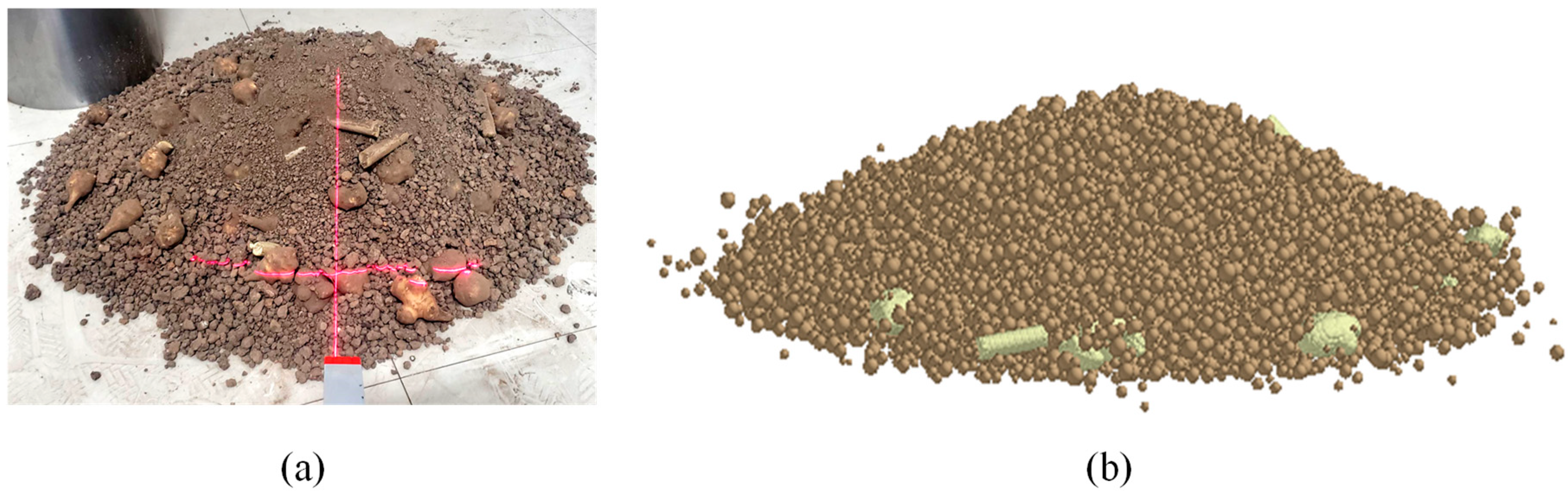
Agriculture 13 01525 g002
Figure 3. Static angle of repose for soil–crop mass calibration: (a) experiment (the red line is a laser pointer which serves as a visual reference for the angle being measured) and (b) DEM simulation.
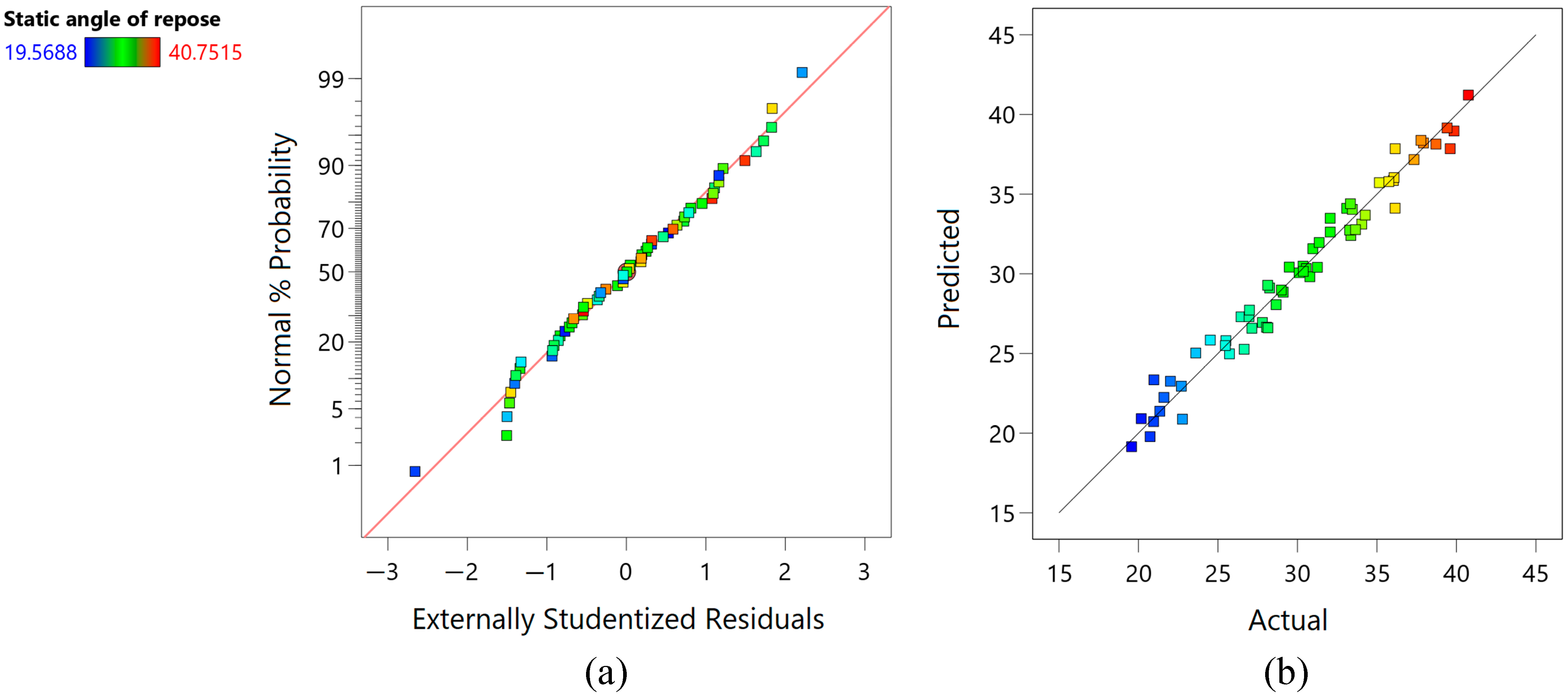
Agriculture 13 01525 g003
Figure 4. Diagnostic plots: (a) normal plot of residuals and (b) predicted versus actual plot.
Agriculture 13 01525 g004
Figure 5. Optimal DEM input parameters from the static angle of repose simulation.
Agriculture 13 01525 g005
Figure 6. DEM crop–modelling technique: (a) Fresh Jerusalem artichoke tuber, (b) 3D computer-aided design model, (c) DEM tuber particle, and (d) DEM crop model.
Agriculture 13 01525 g006
Figure 7. DEM soil–crop mixture model establishment: (a) factory setup, (b) subsoil creation, (c) crop creation, (d) topsoil creation, and (e) soil–crop model.
Agriculture 13 01525 g007
Figure 8. Tractor–harvester setup used in this study.
Agriculture 13 01525 g008
Figure 9. The depth of operation for the two field experiments: (a) clay soil field and (b) sandy loam field.
Agriculture 13 01525 g009
Figure 10. (a) DEM soil–shovel simulation setup, (b) fork-shaped shovel, and (c) S-shaped shovel.
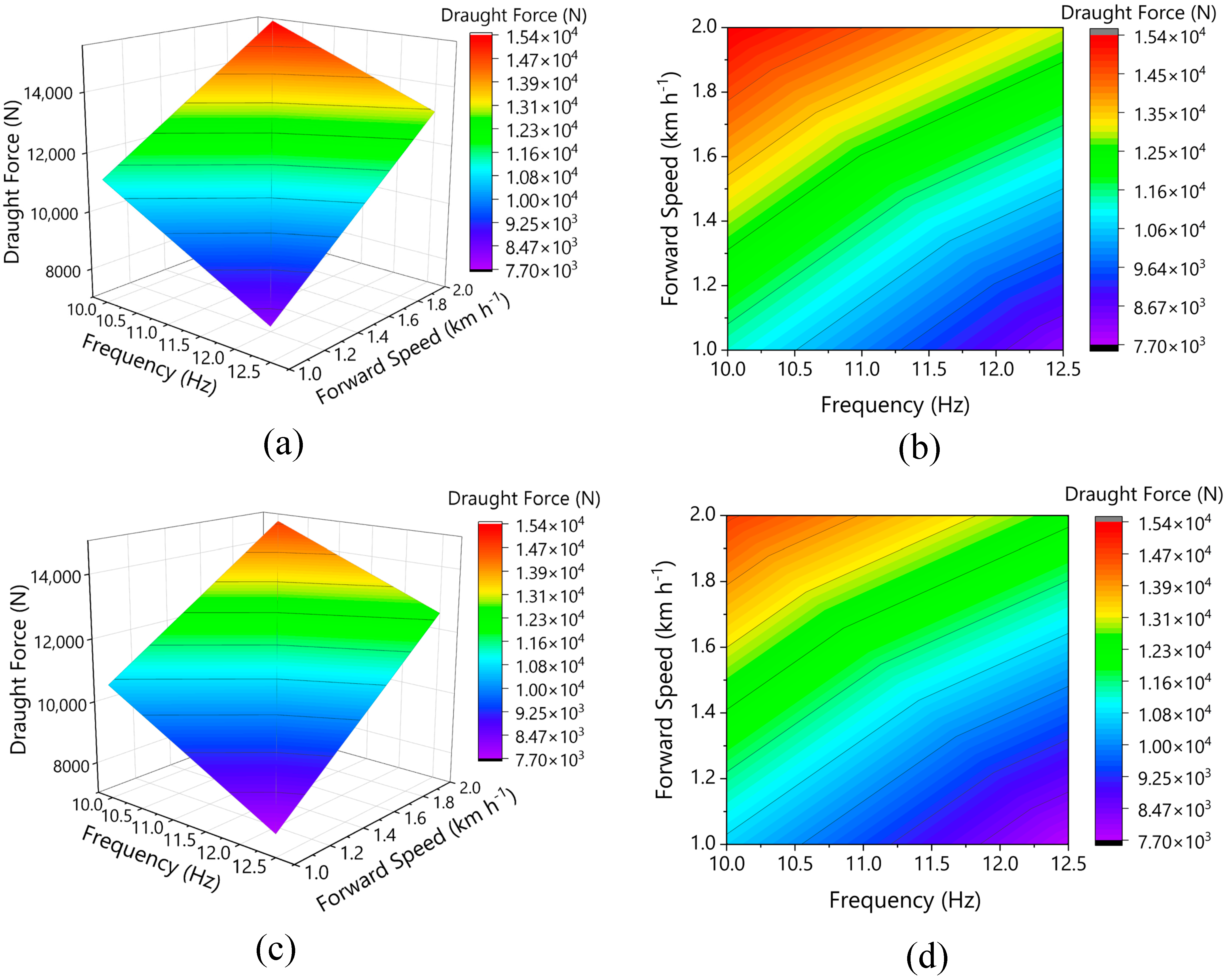
Agriculture 13 01525 g010
Figure 11. Effect of forward speed and vibration frequency on draught force: (a,b) clay field experiment 3D and 2D contour plots, and (c,d) DEM simulation 3D and 2D contour plots.
Agriculture 13 01525 g011
Figure 12. Effects of forward speed and vibration frequency on draught force: (a,b) sandy loam field experiment 3D and 2D contour plots, and (c,d) DEM simulation 3D and 2D contour plots.
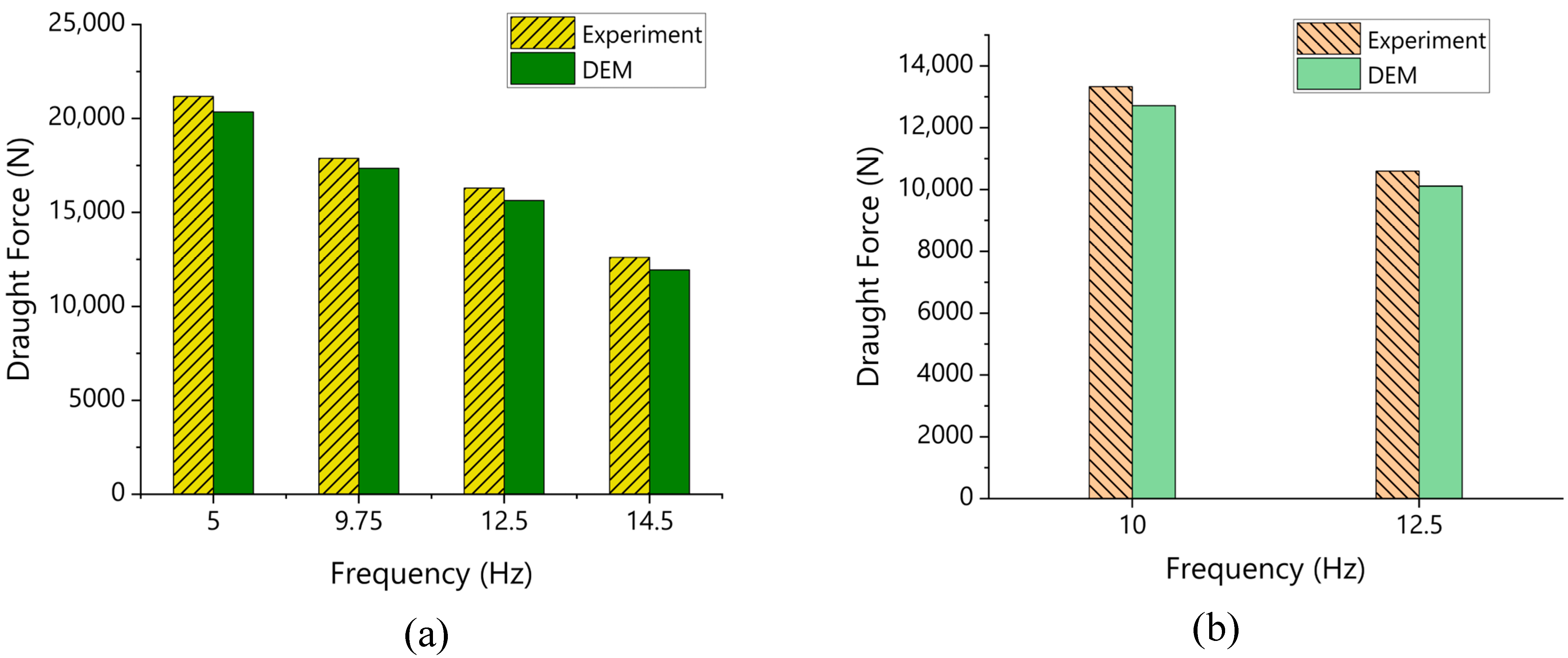
Agriculture 13 01525 g012
Figure 13. Effect of vibration frequency on draught force for the experiment and DEM simulation: (a) clay soil and (b) sandy loam.
Agriculture 13 01525 g013
Figure 14. Comparison of field data and DEM for drawbar power: (a,b) clay soil field and DEM results, respectively; (c,d) sandy loam soil field and DEM results, respectively.
Agriculture 13 01525 g014
Figure 15. Soil translocation properties of the shovels evaluated in clay soil: (a) field experiment for fork shovel, (b) DEM result for fork-shaped shovel, and (c) DEM result for S-shaped shovel.
Agriculture 13 01525 g015
Figure 16. DEM predicted soil bulk density for clay soil evaluation: (a) fork-shaped shovel and (b) S-shaped shovel.
Agriculture 13 01525 g016
Figure 17. Soil–crop mass translocation properties of the tools evaluated in sandy loam soil: (a) field experiment result, (b,c) DEM result for the fork-shaped shovel, and (d,e) DEM result for the S-shaped shovel.
Agriculture 13 01525 g017
Figure 18. DEM-predicted bulk density for sandy loam soil evaluation: (a) fork-shaped shovel and (b) S-shaped shovel.
Agriculture 13 01525 g018
Table 1. DEM input parameters for the soil–crop mixture model (sandy loam soil).
Parameter and UnitValueRemarks
Poison’s ratio: soil0.3Selected
Poison’s ratio: steel0.3[30]
Poisson’s ratio: root0.38Measured
Poison’s ratio: tuber0.48Measured
Poison’s ratio: stem0.35Measured
Particles’ solid density (kg m−3)2600[6]
Density of steel (kg m−3)7865[30]
Density of root (kg m−3)1132Measured
Density of tuber (kg m−3)1184.4Measured
Density of stem (kg m−3)250.75Measured
Shear modulus (Pa): soil 1.7 × 10 7 [6]
Shear modulus (Pa): steel 7.9 × 10 10 [30]
Shear modulus (Pa): root 4.78 × 10 6 Measured
Shear modulus (Pa): tuber 4.23 × 10 6 Measured
Shear modulus (Pa): stem 2.72 × 10 8 Measured
Coefficient of restitution: soil–soil0.6[6]
Coefficient of restitution: soil–steel0.6[6]
Coefficient of restitution: soil–root0.439Calibrated
Coefficient of restitution: soil–tuber0.514Calibrated
Coefficient of restitution: soil–stem0.554Calibrated
Coefficient of restitution: root–steel0.32Measured
Coefficient of restitution: tuber–steel0.62Measured
Coefficient of restitution: stem–steel0.53Measured
Coefficient of static friction: soil–soil0.45[6]
Coefficient of static friction: root–soil0.195Calibrated
Coefficient of static friction: tuber–soil0.212Calibrated
Coefficient of static friction: stem–soil0.166Calibrated
Coefficient of static friction: soil–steel0.45[6]
Coefficient of static friction: root–steel0.511Measured
Coefficient of static friction: tuber–steel0.446Measured
Coefficient of static friction: stem–steel0.5Measured
Coefficient of rolling friction: soil–soil0.18[6]
Coefficient of rolling friction: root–soil0.015Calibrated
Coefficient of rolling friction: tuber–soil0.175Calibrated
Coefficient of rolling friction: stem–soil0.069Calibrated
Coefficient of rolling friction: root–steel0.21Measured
Coefficient of rolling friction: tuber–steel0.32Measured
Coefficient of rolling friction: stem–steel0.05Measured
Normal stiffness per unit area (N m−3) 1 × 10 9 Selected
Shear stiffness per unit area (N m−3) 2.5 × 10 7 Calibrated
Normal strength (Pa) 1.3 × 10 6 Calibrated
Shear strength (Pa) 1.15 × 10 6 Calibrated
Bonded disk scale1Selected
JKR surface energy (J m−2)10Selected
Table 2. DEM input parameters used for the soil–tool interaction simulation (clay soil).
Parameter and UnitValueRemarks
Poison’s ratio: soil0.3Selected
Poison’s ratio: steel0.3[30]
Particles’ solid density (kg m−3)2600Selected
Density of steel (kg m−3)7865[30]
Shear modulus (Pa): soil 2 × 10 7 Calibrated
Shear modulus (Pa): steel 7.9 × 10 10 [30]
Yield strength (Pa): soil (single sphere, dual sphere, and triple sphere) 2.21 × 10 6 , 2.56 × 10 6 ,   a n d   2.37 × 10 6 Default value in EDEM® 2020
Yield strength (Pa): steel 1 × 10 9 Default value in EDEM® 2020
Coefficient of restitution: soil–soil0.467Calibrated
Coefficient of restitution: soil–steel0.05Selected
Coefficient of static friction: soil–soil0.388Calibrated
Coefficient of static friction: soil–steel0.45Selected
Coefficient of rolling friction: soil–soil0.192Calibrated
Coefficient of rolling friction: soil–steel0.15Selected
Damping factor0.5Default value in EDEM® 2020
Stiffness factor0.85Default value in EDEM® 2020
Cohesive energy density (J m−3)20,965.7Calibrated
Table 3. Regression model fit summary for responses (clay field experiment and DEM simulation).
SourceSequential p-ValueAdjusted R2Predicted R2Remark
Experiment draught force
Linear<0.0001 *0.90380.8475
2FI0.0798 **0.92800.7966
Quadratic0.0512 **0.96430.9324Suggested
Cubic0.0340 *0.99470.9664Aliased
DEM draught force
Linear<0.0001 *0.90170.8430
2FI0.0908 **0.92430.7748
Quadratic0.0394 *0.96570.9120Suggested
Cubic0.0240 *0.99590.9538Aliased
Experiment drawbar power
Linear<0.0001 *0.94730.9011
2FI0.0006 *0.98740.9692Suggested
Quadratic0.0963 **0.99230.9734
Cubic0.0085 **0.99950.9977Aliased
DEM drawbar power
Linear<0.0001 *0.94500.8974
2FI0.0010 *0.98500.9623Suggested
Quadratic0.0777 **0.99150.9693
Cubic0.0073 *0.99950.9968Aliased
*: Statistically significant (p < 0.05); **: statistically not significant (p > 0.05).
Table 4. Regression model fit summary for the sandy loam soil (field and DEM simulation).
SourceExperiment Draught ForceDEM Draught Force
Std. Dev.368.33362.5
Mean11,963.111,411.15
CoV%3.083.18
R20.99520.9951
Adjusted R20.98570.9852
Predicted R20.92350.9212
Adequacy precision22.849822.4509
Table 5. ANOVA summary result for the clay soil (field and DEM simulation).
Experiment Draught Force (Quadratic)DEM Draught Force (Quadratic)Experiment Drawbar Power (2FI)DEM Drawbar Power (2FI)
SourceF-Valuep-ValueSourceF-Valuep-ValueSourceF-Valuep-ValueSourceF-Valuep-Value
Model60.51<0.0001 *Model62.89<0.0001 *Model288.85<0.0001 *Model242.23<0.0001 *
A150.65<0.0001 *A159.85<0.0001 *A66.6<0.0001 *A57.390.0003 *
B157.21<0.0001 *B159.02<0.0001 *B810.21<0.0001 *B678.05<0.0001 *
AB8.130.0291 *AB8.150.029 *AB29.720.0006 *AB25.060.0010 *
A25.330.0603 **A27.540.0335 *
B24.830.0.0704 **B24.090.0895 **
Std.Dev.876.40 Std.Dev.836.44 Std.Dev.1.01 Std.Dev.1.06
Mean16,990.08 Mean16,321.74 Mean12.07 Mean11.59
CoV%5.16 CoV%5.12 CoV%8.37 CoV%9.17
A: forward speed; B: frequency; Std.Dev.: standard deviation; CoV: coefficient of variation; 2FI: two-factor interaction; *: statistically significant (p < 0.05); **: statistically not significant (p > 0.05).
Table 6. Comparison of clay soil field and DEM simulation result for draught force and drawbar power.
FrequencyForward SpeedExperiment Draught ForceDEM Draught ForceExperiment Drawbar PowerDEM Drawbar PowerRE
(Hz)(km h−1)(N)(N)(kW)(kW)(%)
5116,542.17015,926.6264.5954.4243.721
5220,951.88920,105.59211.64011.1704.039
5426,036.02225,019.38728.92927.7993.905
9.75113,288.18912,867.7253.6913.5743.164
9.75217,684.54817,270.6549.8259.5952.340
9.75422,677.28421,915.67125.19724.3513.358
12.5112,819.62012,362.9243.5613.4343.562
12.5216,586.87415,699.1749.2158.7225.352
12.5419,479.82118,863.69221.64420.9603.163
14.5110,245.0869795.8352.8462.7214.385
14.5212,573.06311,794.3656.9856.5526.193
14.5414,996.46714,239.18216.66315.8215.050
RE: relative error.
Table 7. Comparison of sandy loam soil field and DEM simulation result for draught force and drawbar power.
FrequencyForward SpeedExperiment Draught ForceDEM Draught ForceExperiment Drawbar PowerDEM Drawbar PowerRE
(Hz)(km h−1)(N)(N)(kW)(kW)(%)
10111,232.58710,669.7303.1202.9645.011
10215,423.26614,753.9718.5688.1974.340
12.518134.5967705.8212.2602.1415.271
12.5213,061.93012,515.0677.2576.9534.187
RE: relative error.
Disclaimer/Publisher’s Note: The statements, opinions and data contained in all publications are solely those of the individual author(s) and contributor(s) and not of MDPI and/or the editor(s). MDPI and/or the editor(s) disclaim responsibility for any injury to people or property resulting from any ideas, methods, instructions or products referred to in the content.

