Research on Provincial-Level Soil Moisture Prediction Based on Extreme Gradient Boosting Model

Abstract

As one of the physical quantities concerned in agricultural production, soil moisture can effectively guide field irrigation and evaluate the distribution of water resources for crop growth in various regions. However, the spatial variability of soil moisture is dramatic, and its time series data are highly noisy, nonlinear, and nonstationary, and thus hard to predict accurately. In this study, taking Jiangsu Province in China as an example, the data of 70 meteorological and soil moisture automatic observation stations from 2014 to 2022 were used to establish prediction models of 0–10 cm soil relative humidity (RH_s10cm) via the extreme gradient boosting (XGBoost) algorithm. Before constructing the model, according to the measured soil physical characteristics, the soil moisture observation data were divided into three categories: sandy soil, loam soil, and clay soil. Based on the impacts of various factors on the soil water budget balance, 14 predictors were chosen for constructing the model, among which atmospheric and soil factors accounted for 10 and 4, respectively. Considering the differences in soil physical characteristics and the lagged effects of environmental impacts, the best influence times of the predictors for different soil types were determined through correlation analysis to improve the rationality of the model construction. To better evaluate the importance of soil factors, two sets of models (Model_{_soil&atmo} and Model_{_atmo}) were designed by taking soil factors as optional predictors put into the XGBoost model. Meanwhile, the contributions of predictors to the prediction results were analyzed with Shapley additive explanation (SHAP). Six prediction effect indicators, as well as a typical drought process that happened in 2022, were analyzed to evaluate the prediction accuracy. The results show that the time with the highest correlations between environmental predictors and RH_s10cm varied but was similar between soil types. Among these predictors, the contribution rates of maximum air temperature (T_amax), cumulative precipitation (P_sum), and air relative humidity (RH_a) in atmospheric factors, which functioned as a critical factor affecting the variation in soil moisture, are relatively high in both models. In addition, adding soil factors could improve the accuracy of soil moisture prediction. To a certain extent, the XGBoost model performed better when compared with artificial neural networks (ANNs), random forests (RFs), and support vector machines (SVMs). The values of the correlation coefficient (R), root mean square error (RMSE), mean absolute error (MAE), mean absolute relative error (MARE), Nash–Sutcliffe efficiency coefficient (NSE), and accuracy (ACC) of Model_{_soil&atmo} were 0.69, 11.11, 4.87, 0.12, 0.50, and 88%, respectively. This study verified that the XGBoost model is applicable to the prediction of soil moisture at the provincial level, as it could reasonably predict the development processes of the typical drought event.

1. Introduction

Soil moisture is a critical climate variable that regulates climate change by facilitating the exchange and distribution of water and energy in land–air interaction. Additionally, soil moisture plays a significant role in agricultural production, as deficits or overflows of soil moisture during critical periods can impact crop growth and yields [1]. Integrating information on available soil moisture and crop water demands can help the development of timely and appropriate irrigation schedules [2], which is particularly important in areas with poor water conditions.

The variations and differences in soil moisture across regions are determined by its budget balance, which is influenced by several factors. Soil moisture is sourced from atmospheric precipitation and artificial irrigation, and its expenditure depends on physical processes such as evapotranspiration and runoff, which are influenced by local weather conditions, soil characteristics, land cover, and other factors [3]. Usually, soil moisture can be expressed using physical variables such as relative humidity, weight water content, and volume water content. Among these variables, relative humidity, calculated as the percentage of soil water content and field capacity, can comprehensively reflect the soil moisture status and surface hydrological processes [4,5]. Consequently, soil relative humidity is an essential reference in irrigation, enabling an analysis of soil moisture differences between regions. Soil moisture prediction based on relative humidity can enhance the defense against waterlogging and drought in farmland.

Numerous studies have investigated soil moisture prediction using various methods. Traditional approaches include the water balance method [6,7,8], statistical empirical formula method [9], time series method [10,11], and physical models based on hydrological processes [12]. These methods typically consider the soil water budget balance principle, relationships between soil water and environmental factors, change characteristics of soil water over time, and land–air interaction. They use model building or time series analysis to forecast soil moisture. With advances in information technology, various applications of machine learning (ML) in agricultural production have been widely developed, including predictions of the crop growth period, yield, and soil moisture [13,14,15,16]. ML technologies such as artificial neural networks (ANNs) [17], support vector machines (SVMs) [18], and gradient boosting regression trees (GBRTs) [19] offer a novel perspective for soil moisture prediction due to their advantages of having a low computational cost, strong self-learning ability, high prediction accuracy, and wide suitability [20,21,22]. For instance, a GA-BP neural network regression model was tested to perform well in predicting the soil moisture of high side slopes [23]. A proposed novel encoder–decoder model with residual learning played an excellent role in solving the nonlinear problem of soil moisture prediction, which was tested using data from 13 FLUXNET sites with varying plant function types and climatic characteristics [24].

In the research of soil moisture prediction based on machine learning, besides finding suitable prediction models [25], selecting the appropriate input factors for the prediction model is crucial. Many studies have selected meteorological factors directly related to soil moisture, such as precipitation, transpiration, sunshine, and surface temperature [26]. For instance, Xu et al. (2010) developed and tested an integrated soil moisture prediction model based on artificial neural networks (ANNs) with meteorological data in the semi-arid region of eastern China, and the model performed well at basin scales [27]. Li et al. (2018) applied the adaptive genetic ANN method to improve the quality of soil moisture prediction using atmospheric forcing data, which include air temperature, relative humidity, wind speed, radiation, and precipitation, as well as soil forcing data, such as soil temperature at 5 cm depth and lagged soil moisture at 0–10 cm [28]. Moreover, with the advancement of remote sensing technology, remote sensing monitoring indexes based on multi-source data, including optical, thermal infrared, microwave, and other data, have also been widely used for soil moisture monitoring and prediction [29,30,31].

However, current research on soil moisture prediction has some limitations, including discontinuity in remote sensing images, an inadequate use of data from automatic observation stations, and unclear influencing factors of soil moisture [24,32]. Therefore, this study utilized the soil moisture data and corresponding meteorological data from 70 automatic stations in Jiangsu Province, determined the optimal influence times of the input factors for prediction models using a correlation analysis method, and applied extreme gradient boosting (XGBoost) to establish two sets of soil relative humidity prediction models (i.e., Model_{_soil&atmo} and Model_{_atmo}). To better interpret the influences of the input factors on these two models and evaluate their performance, Shapley additive explanation (SHAP) was applied, and six metrics were utilized as the predicting effect indicators to compare the models’ (e.g., ANN, RF, and SVM) prediction accuracy. Furthermore, a typical drought development process in August 2022 in Jiangsu Province was analyzed in depth. This study aimed to establish a provincial-level and understandable soil moisture prediction model by applying a machine learning algorithm, which could provide a case study for other regions.

2. Materials and Methods

2.1. Study Area

Jiangsu Province (see Figure 1) is located on the east coast of China, in the mid-latitude zone, with a geographical location between 30°46′–35°07′ N and 116°22′–121°55′ E. It lies in the climate transition zone between the subtropical and warm temperate zones and belongs to the East Asian monsoon climate zone. The average annual temperature, precipitation, and sunshine hours in Jiangsu Province are between 13.6–16.1 °C, 704–1250 mm, and 1816–2503 h, respectively [33]. The terrain is generally flat, with the Taihu Plain, Yanjiang, and Lixia River areas being low-lying and having dense water networks. The low mountains and hills account for only 14.33% and are mainly distributed in the west and north regions. There are various soil types in Jiangsu, including zonal soils such as cinnamon, brown soil, yellow-brown soil, and yellow soil, and non-zonal soils such as saline soil, meadow soil, and marsh soil. With a long history of agriculture, natural soil in Jiangsu has evolved into various types of farming soil with different soil textures under the influence of different farming systems and utilization methods [34].

2.2. Data Source

Automatic moisture observation instruments have been gradually incorporated into the meteorological operational observation system since 2010, resulting in the availability of high regional density and continuous soil moisture observation data across Chinese provinces [35]. Consequently, daily 0–10 cm soil relative humidity data, measured by 70 automatic soil moisture observation stations in Jiangsu Province from 2014 to 2022, along with meteorological data collected by automatic weather stations and soil temperature data measured by soil temperature instruments at the corresponding 70 soil moisture station locations, were used for predicting 0–10 cm soil relative humidity. These atmospheric and soil observation data were obtained from the Jiangsu Meteorological Information Center.

Based on the principle of soil water budget balance and considering the influence of various factors on the 0–10 cm soil relative humidity (RH_s10cm, %), the predictive factors were divided into two categories: atmospheric and soil factors. There are ten atmospheric factors, including the mean air temperature (T_a, °C), minimum air temperature (T_amin, °C), maximum air temperature (T_amax, °C), air relative humidity (RH_a, %), precipitation (P, mm), sunshine hours (S, h), wind speed (W, ms⁻¹), atmospheric pressure (P_r, hPa), water vapor pressure (e, hPa), and potential evapotranspiration (ET₀, mm). Additionally, there are four soil factors, including the mean surface temperature (T_s, °C), maximum soil surface temperature (T_smax, °C), minimum soil surface temperature (T_smin, °C), and 0–10 cm soil temperature (T_s10cm, °C).

2.3. Data Classification

Soil textures and hydrological constants varied significantly in Jiangsu Province. Even when weather conditions are identical, different regions may exhibit distinct soil water dynamics due to the differences in soil physical properties [36]. Therefore, it is necessary to consider regional soil characteristics and hydrological constants when predicting soil moisture. To this end, according to the soil hydrological and physical characteristics measured by 70 automatic soil moisture observation stations in Jiangsu Province, the soil moisture observation data were classified into three categories: sandy soil, loam soil, and clay soil. The statistics of physical parameters corresponding to the different soil types are shown in

Table 1. Classification results and corresponding soil physical characteristics of soil moisture observation data.

Soil Type	Soil Bulk Density (g·cm−3)	Field Water Capacity (%)	Withering Humidity (%)	Samples
Sand	1.43	25.46	4.04	40,880
Loam	1.40	26.50	5.29	75,920
Clay	1.36	26.62	5.72	87,600

.

2.4. Methodology Description

2.4.1. Selection of Predictive Factors

Soil relative humidity changes are mainly affected by previous and current weather conditions and the state of the soil itself. By distinguishing different soil types, we correlated RH_s10cm with the averaged or accumulated value (including precipitation and sunshine hours) of 14 predictor factors on the same day as the soil moisture observed, and 1–10 days in the previous period, to determine the maximum impact time of each predictor (see

Table 2. List of predictor factors of 0–10 days prior, which are used for correlation analysis with RH_s10cm.

Names	Units	Descriptions	Range
Sunshine hours	h	Accumulated sunshine hours	0–128.6
Precipitation	mm	Cumulative precipitation	0–595.4
Evapotranspiration	mm	Averaged potential evapotranspiration	0.1–10.2
Wind speed	ms−1	Averaged wind speed	0–15.9
Relative humidity	%	Averaged mean air relative humidity	19–100
Pressure	hPa	Averaged water vapor pressure	0.6–42.0
		Averaged atmospheric pressure	983.5–1042.4
Temperature	°C	Averaged mean air temperature	−11.1–36.0
		Averaged minimum air temperature	−15.6–31.9
		Averaged maximum air temperature	−7.2–40.9
		Averaged mean soil surface temperature	−7.0–45.8
		Averaged minimum soil surface temperature	−14.7–31.2
		Averaged maximum soil surface temperature	−0.9–70.2
		Averaged 0–10 cm mean soil temperature	−2.7–39.0

). We used the time with the largest correlation coefficient of each predictor as its maximum impact time on RH_s10cm. The corresponding sample numbers for each soil type used to take correlation analysis are shown in Table 1.

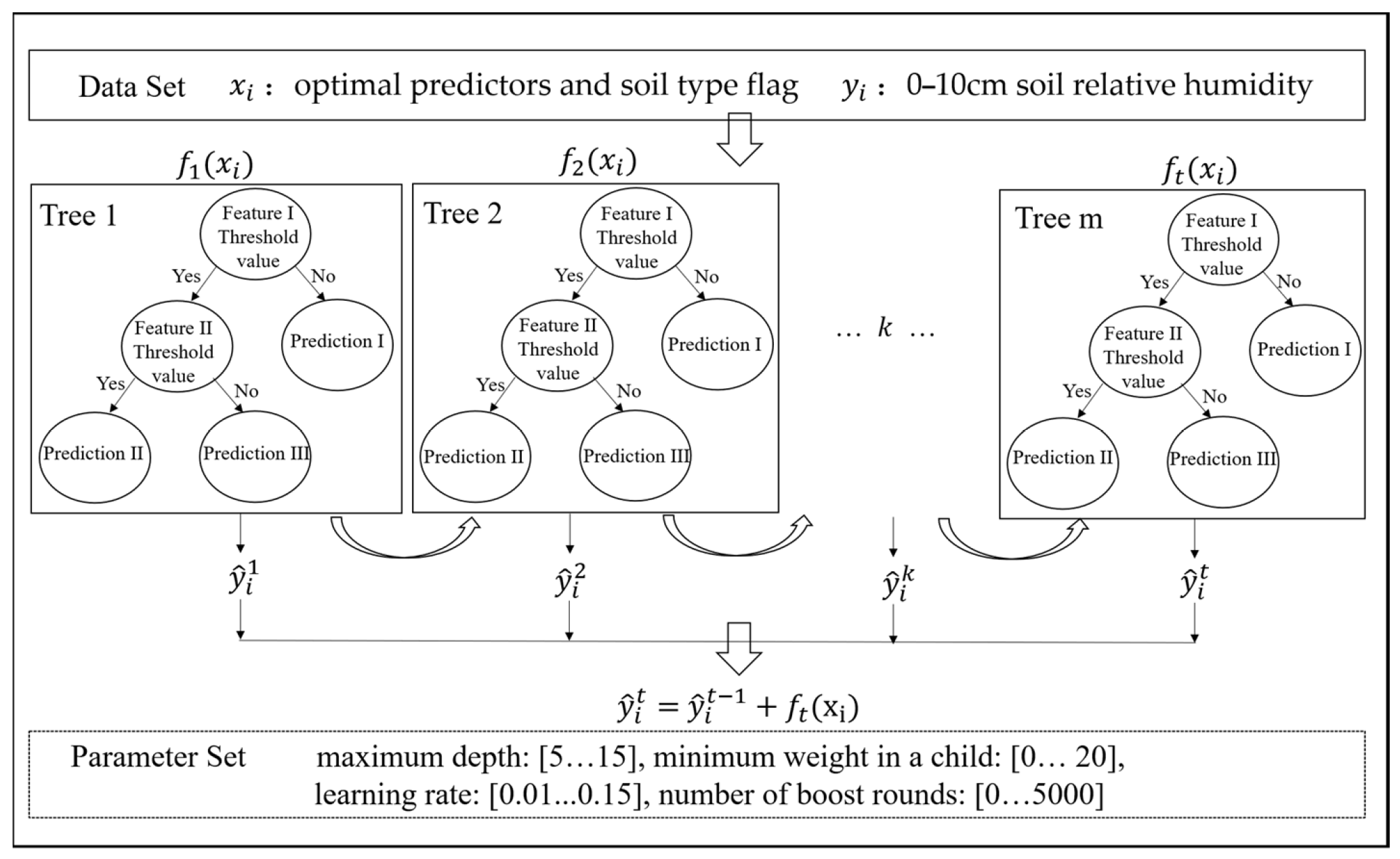
2.4.2. XGBoost Model

The XGBoost is an ensemble learning method based on boosting [37]. The boosting technique combines multiple decision trees and aggregates their predictions to obtain a final prediction that is more accurate than any individual tree. XGBoost is designed to prevent over-fitting. The XGBoost model builds multiple trees sequentially, with each subsequent tree intended to reduce the errors of the previous tree. As the training proceeds iteratively, new trees are added to predict the error of the prior tree. Such a fitting process is repeated several times until a stopping criterion is met, such as when the root mean square error (RMSE) reaches an asymptotic value. The ultimate prediction of the model is the sum of the predictions from all of the trees. The formula for the prediction at the step $t$ and site location $i$ can be defined as follows [37]:

$${\widehat{y}}_i^t={\displaystyle {\sum }_{k=1}^t{f}_k}(x_i)={\widehat{y}}_i^{(t-1)}+f_t(x_i)$$

(1)

where $f_t(x_i)$ is the tree model at step $t$, ${\widehat{y}}_i^t$ and ${\widehat{y}}_i^{(t-1)}$ are the predictions at steps $t$ and $t-1$, and $x_i$ are the predictor variables. The parameters of the model $f(x_i)$ are selected by optimizing the objective function, and the objective function is defined by root mean square error.

Additionally, XGBoost offers several other advanced features [37] that can further enhance the model’s performance. For instance, early stopping allows the training process to be stopped early if the performance on a validation set stops improving. This advanced feature prevents the model from overfitting to the training data and can improve its ability to generalize to new data. Cross-validation is another useful technique that can estimate the model’s generalization performance and help to select the optimal hyperparameters. By incorporating these and other advanced features, XGBoost has emerged as one of the most popular and influential machine learning models. The flow chart depicting the XGBoost model is presented in Figure 2.

2.4.3. The Key Parameters of XGBoost Model

In this study, we focused on optimizing several crucial parameters of the XGBoost algorithm, including the number of boost rounds, maximum depth, minimum weight in a child, and learning rate. The number of boost rounds determines the maximum number of boosting iterations, while the maximum depth sets the maximum depth of an individual tree. The minimum weight in a child parameter is utilized to prevent overfitting, and the learning rate parameter controls the model’s shrinkage at every step (i.e., a lower learning rate indicates more steps used to achieve the optimum) (see Figure 2).

To optimize these parameters, we applied a tuning technique called grid search [38]. This approach computes the optimal values of hyperparameters by exhaustively searching over a range of possible parameter values. We utilized third-fold cross-validation [39] to evaluate the performance of different parameter combinations. In total, we searched through 1500 combinations of parameter values. Ultimately, our XGBoost model achieved the best performance with the maximum depth, minimum weight needed in a child, and learning rate equal to 15, 10, and 0.02, respectively. In addition, we set the maximum number of boosting rounds to 5000 during training and used the early stop technique to stop the training. The final number of iterations was 4218 when the loss on the validation set no longer decreased.

2.4.4. Shapley Additive Explanations (SHAPs)

SHAP is a local attribution method that is based on the use of Shapley values. The Shapley values originate from the field of cooperative game theory and represent each play’s average expected marginal contribution in a cooperative game after all possible combinations of players have been considered. It can be formulated as follows [40]:

$${\varphi }_i={\displaystyle \sum _{S\subseteq F\backslash \left\{i\right\}}\frac{\left|S\right|!(F-\left|S\right|-1)!}{F!}[f_x(S\cup \{i\})-f_x(S)]}$$

(2)

where ${\varphi }_i$ is the weighted average of all marginal contributions of the predictor $i$, $F$ is the total number of features, $S$ is the subset of predictors from all predictors except for predictor $i$, and $\frac{\left|S\right|!(F-\left|S\right|-1)!}{F!}$ is the weighting factor counting the number of permutations of the subset $S$. $f_x(S)$ is the expected output given the predictors subset $S$. $[f_x(S\cup \left\{i\right\})-f_x(S)]$ is the difference made by the predictor $i$.

2.4.5. Model Construction and Application

This study aimed to develop a soil moisture prediction model for different soil types using relevant atmospheric and soil factors. To achieve this, 14 most related factors were obtained by calculating the correlation. Additionally, to account for the different impacts of soil types, the variable St_flag was included in the model, with values of 1, 2, and 3 representing sandy, loam, and clay soils, respectively.

To further evaluate the importance of soil factors in predicting 0–10 cm soil relative humidity, two sets of data used as the model’s independent variables were constructed using 14 optimal predictors (including atmospheric and soil variables) and 10 optimal predictors (including atmospheric variables only) from 70 stations in Jiangsu Province between 2014 and 2021. Before prediction, missing values in these two data sets were completed with the mean values, and the dataset was normalized. A tri-fold cross-validation approach [39] was employed to train, validate, and evaluate the model. The data were randomly divided into three sets: 80% (163,520 samples) as the model training dataset, 10% (20,440 samples) as the model validation dataset for parameter optimization, and the remaining 10% (20,440 samples) as the model prediction evaluating dataset.

2.4.6. Model Prediction Effect Interpretation and Verification

After building the prediction model, the SHAP method was applied to obtain each predictive factor’s positive and negative effects separately for both Model_{_soil&atmo} and Model_{_atmo}. In addition, six metrics were used on the evaluating dataset to evaluate the performance of XGBoost and other state-of-the-art predictive models, including correlation coefficient (R), root mean square error (RMSE), mean absolute error (MAE), mean absolute relative error (MARE), Nash–Sutcliffe efficiency coefficient (NSE), and accuracy (ACC). These indicators are calculated as follows [41]:

$$\mathrm{R}=\frac{{\displaystyle \sum _{i=1}^n(y_i-{\overline{y}}_i)({\widehat{y}}_i-{\overline{\widehat{y}}}_i)}}{\sqrt{{\displaystyle \sum _{i=1}^n{(y_i-{\overline{y}}_i)}^2{\displaystyle \sum _{i=1}^n{({\widehat{y}}_i-{\overline{\widehat{y}}}_i)}^2}}}}$$

(3)

$$\mathrm{RMSE}=\sqrt{\frac{{\displaystyle \sum _{i=1}^n{(y_i-{\widehat{y}}_i)}^2}}{n}}$$

(4)

$$\mathrm{MAE}=\frac{1}{n}{\displaystyle \sum _{i=1}^n\left|(y_i-{\widehat{y}}_i)\right|}$$

(5)

$$\mathrm{MARE}=\frac{1}{n}{\displaystyle \sum _{i=1}^n\left|\frac{(y_i-{\widehat{y}}_i)}{y_i}\right|}$$

(6)

$$\mathrm{NSE}=1-\frac{{\displaystyle \sum _{i=1}^n{(y_i-{\widehat{y}}_i)}^2}}{{\displaystyle \sum _{i=1}^n{({\widehat{y}}_i-\frac{{\displaystyle \sum _{i=1}^n{y}_i}}{n})}^2}}$$

(7)

$$\mathrm{ACC}=1-\frac{1}{n}{\displaystyle \sum _{i=1}^n\left|\frac{(y_i-{\widehat{y}}_i)}{y_i}\right|}\ast 100\%$$

(8)

where $y_i$ is the observed value, ${\widehat{y}}_i$ is the predicted value, n is the number of samples, ${\overline{y}}_i$ is the mean of observations, and ${\overline{\widehat{y}}}_i$ is the mean of the prediction.

To further verify the prediction capabilities of Model_{_soil&atmo} and Model_{_atmo} based on XGBoost, we compared these models with three state-of-the-art machine learning models (i.e., ANN [42], RF [43], and SVM [44]) for soil moisture prediction over 70 sites in Jiangsu. The comparison was based on the values of these above metrics and the scatter distributions of predicted and observed soil moisture values. Furthermore, we evaluated the performance of Model_{_soil&atmo} and Model_{_atmo} during a typical drought in August 2022 in Jiangsu Province. The flow chart depicting the establishment, interpretation, and evaluation of the prediction models for soil moisture is presented in Figure 3.

3. Results

3.1. Correlation Analysis between Soil Moisture and Predictive Factors

After analyzing the correlations between 0–10 cm soil relative humidity (RH_s10cm) and various predictors for different soil types with different advance days (See Figure 4), it was observed that, among the atmospheric factors, RH_s10cm had a high positive correlation with the mean air relative humidity (RH_a) and cumulative precipitation (P_sum). The correlation coefficients were between 0.17–0.33 and 0.13–0.26, respectively, and their absolute values gradually increased with the leading time, peaking 8–10 days prior. Additionally, RH_s10cm had a high negative correlation with the mean water vapor pressure (e) and accumulated sunshine hours (S_sum). The absolute correlation coefficients were between 0.24–0.33 and 0.15–0.33, respectively. The absolute values also increased with the leading time, reaching the maximum at 8 and 10 days prior, respectively. Among the soil factors, RH_s10cm had a high negative correlation with the mean maximum surface temperature (T_smax), with its maximum absolute value appearing 4–5 days prior. The correlations between RH_s10cm and other factors were relatively low, but all passed the significance test of $p=0.01$.

Overall, the correlations between RH_s10cm and various predictor factors, as well as their change rules with the days advanced, were relatively consistent among different soil types, with the times taken to reach the maximum value being similar (see Figure 4a–c). The variabilities of positive–negative correlation with RH_s10cm were mainly reflected in the factors of the minimum surface temperature and wind speed. Thus, a fixed optimal impact time was set for each predictor factor as the model input, and its corresponding differences in the impact times between different soil types were no longer distinguished.

3.2. Interpretability of Model

We analyzed the relationships between the predictor variables and the soil moisture using the XGBoost model and presented the results through SHAP summary plots for each variable. In Figure 3, for each predictor variable displayed on the y-axis, each colored point represents a value of this variable in the dataset and the SHAP values displayed on the x-axis denoting the contributions of that predictor variable, which can be a positive or negative effect on the prediction of soil moisture. The gradient color of each point indicates the value of the predictor variable, ranging from low (blue) to high (red), providing a visual representation of the relationships between the predictors and soil moisture.

From the SHAP summary chart of Model_{_soil&atmo} in Figure 5a, we observed that T_smax, T_s10cm, and T_amax had a significant negative contribution to the model prediction, considering both atmospheric and soil variables. Conversely, the effects of other factors on the prediction results were either opposite or insignificant. Among them, P_sum had the most considerable positive contribution to the model prediction, followed by RH_a. According to the importance of each predictor, the order of the top five predictors was T_smax > P_sum > T_s10cm > RH_a > T_s.

From the SHAP summary chart of Model_{_atmo} in Figure 5b, we found that the greater value of T_amax, e, and W had a greater negative contribution to the model prediction, considering only atmospheric variables. In contrast, other factors have opposite effects on the prediction results, or their positive–negative characteristics were insignificant. Among them, P_sum had the most significant positive contribution to the model prediction, followed by RH_a, which was consistent with the results of Model_{_soil&atm}. According to the importance of each predictor, the order of the top five predictors was P_sum > T_amax > RH_a > e > W.

3.3. Model Prediction Evaluation

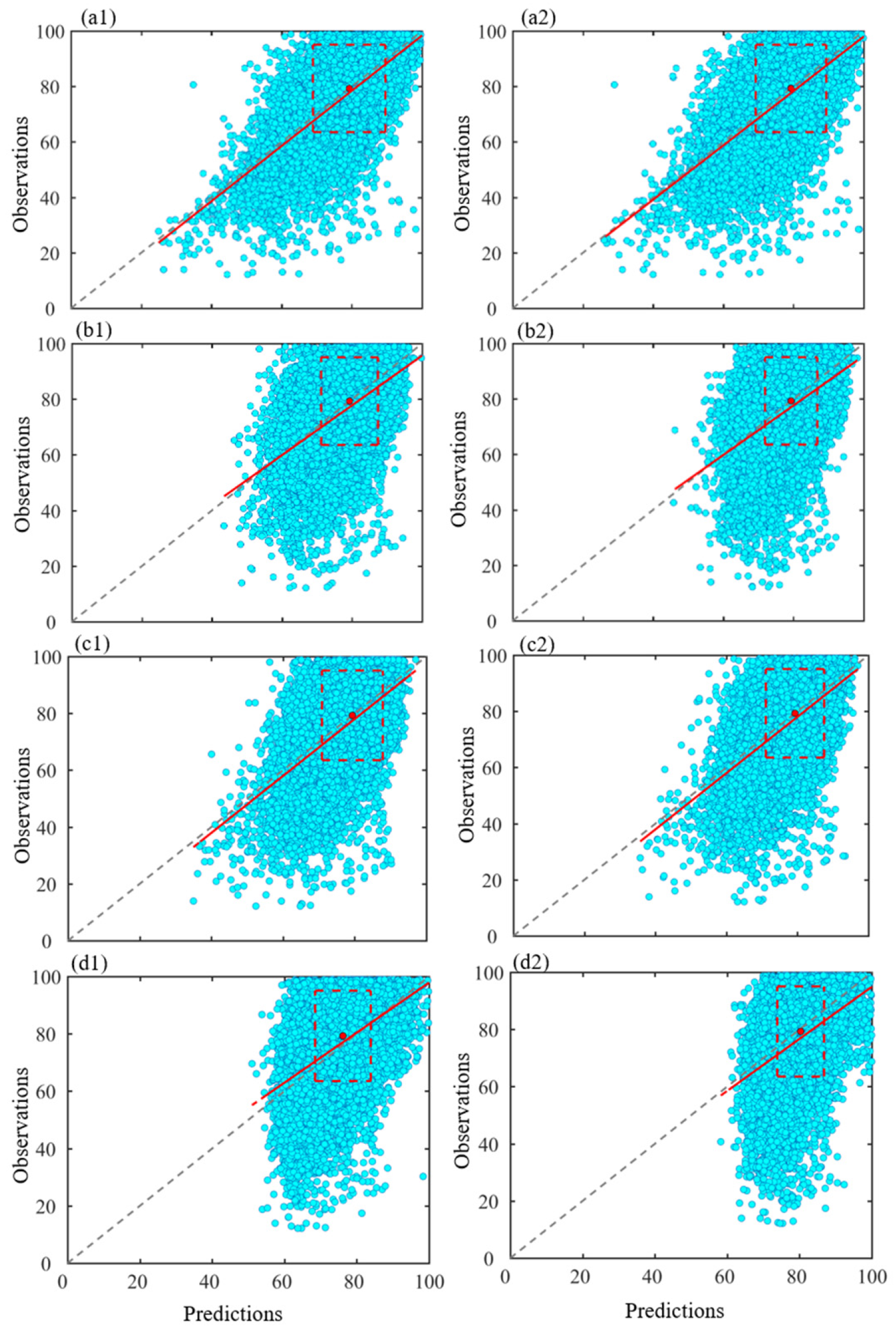
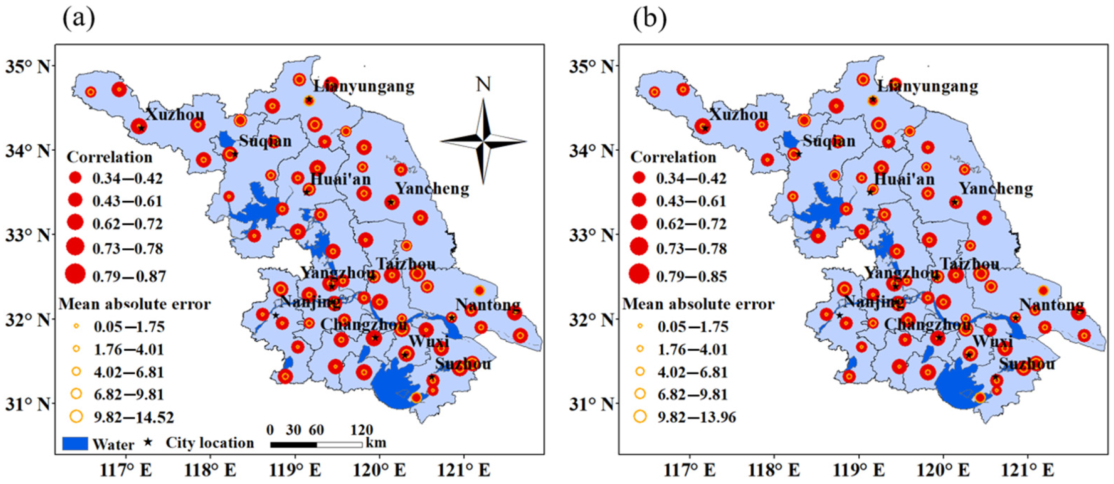
3.3.1. Analysis of Model Prediction Accuracy

To further verify the prediction capabilities of Model_{_soil&atmo} and Model_{_atmo} based on XGBoost, we compared them with three other state-of-the-art machine learning models (i.e., ANN, RF, and SVM) based on the scatter distributions of the predicted and observed values of soil moisture, and the values of six metrics (i.e., R, RMSE, MAE, MARE, MSE, and ACC).

The scatter distributions of the model predictions based on XGBoost and the actual observations of the 0–10 cm soil relative humidity are presented in Figure 6a1,a2. Model_{_soil&atmo} and Model_{_atmo} showed an even distribution of predicted and observed values around the 1:1 diagonal, with Model_{_soil&atmo} exhibiting a slightly more clustered distribution. The mean and standard deviation of Model_{_soil&atmo} ’s predictions (79.28% and 10.32%, respectively) were similar to those of the observations (79.30% and 15.77%, respectively). Model_{_atmo} ’s prediction results were comparable to those of Model_{_soil&atmo}, with only minor differences. However, overall, the prediction performance of Model_{_soil&atmo} was slightly better than that of Model_{_atmo}.

After comparing the scatter distributions of observations with model predictions based on XGBoost, ANN, RF, and SVM (see Figure 6), it was observed that the lines between the predicted and observed soil moisture for XGBoost were much closer to the ideal line (y = x) than those for the other predictive models. Additionally, the prediction results of the other models presented a relatively smaller standard deviation.

Table 3. Comparison of XGBoost, ANN, RF, and SVM performances in soil moisture prediction using two data sets as the model’s input.

ML	Models	R	RMSE	MAE	MARE	NSE	ACC (%)
XGBoost	Model_soil&atmo	0.69	11.11	4.87	0.12	0.50	88%
	Model_atmo	0.66	11.49	4.96	0.14	0.47	86%
ANN	Model_soil&atmo	0.59	12.85	6.55	0.16	0.27	84%
	Model_atmo	0.56	13.19	6.71	0.17	0.23	83%
RF	Model_soil&atmo	0.64	12.08	6.07	0.15	0.36	85%
	Model_atmo	0.63	12.25	6.19	0.16	0.34	84%
SVM	Model_soil&atmo	0.54	13.68	7.56	0.17	0.19	83%
	Model_atmo	0.51	13.58	6.86	0.18	0.18	82%

shows the comprehensive predictive performances of XGBoost, ANN, RF, and SVM over 70 sites in Jiangsu Province. The values of R, RMSE, MAE, MARE, NSE, and ACC for Model_{_soil&atmo} and Model_{_atmo} based on XGBoost were 0.69, 11.11, 4.87, 0.12, 0.50, and 88%, as well as 0.66, 11.49, 4.96, 0.14, 0.47, and 86%, respectively. Comparing the values of the six evaluated indexes of other LM models, it was found that models based on XGBoost always had the lowest RMSE, MAE, and MARE, as well as the highest R, NSE, and ACC.

In addition, for XGBoost, compared with Model_{_atmo} having an average prediction accuracy of 86%, Model_{_soil&atmo} had better precision, with an average accuracy of 88%. Notably, Model_{_soil&atmo}’s prediction effects were always slightly better than those of Model_{_atmo}, which was also evident from the prediction results of other models, whether from the scatter charts or metrics.

Furthermore, the spatial distribution map of the model evaluation indexes (i.e., R and MAE) showed that both Model_{_soil&atmo} and Model_{_atmo} based on XGBoost had a high accuracy in soil moisture prediction, and their spatial distribution patterns were very similar, with differences only at individual stations (see Figure 7). Stations with relatively small correlation coefficients and large average absolute errors of predictions and observations of both models were mainly concentrated along the northern area of the Yangtze River and in the northeastern area of Jiangsu Province.

In addition, we found that the prediction accuracy of both models varied greatly between sites from the spatial distribution maps. According to the statistical analysis, for Model_{_soil&atmo}, the R between the predicted and measured values ranged from 0.34 to 0.87, with a mean value of 0.69, and the MAE ranged from 0.12% to 14.52%, with a mean value of 4.87%. The number of sites with R > 0.60 reached 58, accounting for more than 82%, and the number of sites with MAE < 5% reached 40, accounting for more than 57%. For Model_{_atmo}, the R between the predicted and measured values ranged from 0.34 to 0.85, with an average value of 0.66, and the MAE ranged from 0.05% to 13.96%, with an average value of 5.04%. The number of sites with R > 0.60 reached 53, accounting for more than 75%, and the number of sites with MAE < 5% reached 38, accounting for more than 50%.

3.3.2. Analysis of Typical Drought Process

During 2–23 August 2022, a third round of persistent high temperature occurred in Jiangsu Province, with the first two rounds taking place on 16–22 June and 8–15 July, respectively. The south of Huaihe region experienced 14–19 days of a maximum temperature ≥ 37 °C, with the average temperature between 32–33.7 °C. Compared to the same period in a normal year, the temperature in 2022 was approximately 4 °C higher and the precipitation was less than 90%. In particular, southern Jiangsu faced widespread high temperatures above 40 °C from 12–15 August, resulting in a rapid expansion of drought across the province. By 15 August, most of the southern Huaihe Basin experienced moderate or above meteorological drought, with some areas suffering from severe drought. However, the high temperature gradually receded from 24 August, and the precipitation gradually increased, mainly in the Huaibei and Sunan areas. As a result, the moisture conditions across the province improved effectively, and the moisture content reached an appropriate level.

According to the distribution of a 0–10 cm soil relative humidity on 1, 15, and 30 August, which was interpolated from the measurement of the automatic soil moisture station (see Figure 8a1–a3), we found on 1 August, affected by antecedent precipitation, the soil moisture in most areas of northern Jiangsu was saturated, and the field humidity was relatively high, while the 0–10 cm soil relative humidity in some areas of southern Jiangsu was less than 60%. By 15th August, there was a severe soil water shortage in most of the southern Huaihe Basin. The 0–10 cm soil relative humidity was only 40% to 50%, which had reached moderate drought, and was even less than 40% in some regions, reaching severe drought. Affected by precipitation, by 30 August, the field soil humidity in some areas of Huaibei was relatively high, and the 0–10 cm soil relative humidity in most southern Huaihe Basin had generally improved to more than 60%, with only sporadic areas still suffering from the drought. Thus, it can be seen that the variation in farmland drought perfectly corresponds with the beginning, aggravation, and extinction of the entire high-temperature process.

The spatial distribution patterns of the corresponding prediction results of the models agreed with the observation results. The prediction results reflected not only the development process of drought but also the distribution areas of different levels of farmland drought. However, the predicted drought situation was relatively weak compared to the observation results. Overall, the differences in the distribution pattern and numeric value between the predictions and observations of Model_{_soil&atmo} were less than those of Model_{_atmo} (see Figure 8b1–b3 and Figure 8c1–c3, respectively).

4. Discussion

Based on the observation, soil types, and meteorological data, this study adopted XGBoost to predict soil moisture variations. Different atmospheric and soil factor combinations were selected as input variables to establish two sets of prediction models (Model_{_soil&atmo} and Model_{_atmo}) for RH_s10cm. At the same time, the contributions of the predictive factors were discussed using SHAP. The prediction accuracy was evaluated by comparing six evaluated indexes with other popular ML methods and analyzing a typical drought process in 2022.

The variation in soil moisture is a complex coupling system that exhibits high noise, nonlinearity, and unstable random time series data [22]. Compared to traditional statistical models, machine learning algorithms use multiple processing layers consisting of complex structures or multiple nonlinear transformations to highly abstract data, which could overcome the influence of white noise on the prediction accuracy and effectively improve the simulation accuracy [25]. However, different ML methods have different applicabilities for the same dataset. For example, in a study predicting soil moisture based on three different datasets, machine learning techniques such as multiple linear regression (MLR), support vector regression (SVR), and recurrent neural networks (RNNs) were compared, and MLR was found to have a better performance than the others. Our study used automatic soil moisture observations to compare the prediction accuracies of two models based on XGBoost with ANN, RF, and SVM. It showed that Model_{_soil&atm} based on XGBoost was superior, providing the lowest RMSE (11.11), MAE (4.87), and MARE (0.12), and highest R (0.69), NSE (0.50), and ACC (88%). Due to different research and application purposes, the dataset applied in soil moisture prediction studies based on machine learning algorithms is varied, including in situ sites [45], remote sensing [46], reanalysis [47], and flux stations [24]. These datasets usually belong to diverse regions with different spatial and temporal resolutions, so it is still challenging to make direct comparisons even if the same method is applied.

The analysis of a typical drought process showed that the XGBoost model based on site data had a good performance and was a feasible method for soil water content prediction, as it could capture a reasonable spatial distribution of the soil moisture. In addition, several advantages were considered for choosing the data observed from the automatic observation stations. Firstly, for a specific site, the data of the automatic observation station have lower errors than the data obtained by remote sensing instruments and reanalysis data, where the problems of insufficient time resolution and delayed acquisition also exist [47]. Hence, we can more accurately explore the relationship between soil moisture and environmental parameters. Secondly, soil moisture and its related meteorological or soil data are commonly available with the exact temporal resolution, so abundant data could be provided for training the predictive model. It is important to note that the predictivity of soil moisture depends on the data’s time steps and spatial resolutions due to their different distribution and variation [24,48]. Moreover, the wideness of the application of soil moisture prediction usually depends on its spatial representativeness. Therefore, as more automatic weather stations are installed, the proposed model based on site data could be helpful for the operational studies on soil moisture prediction over larger regions and could provide information for timely and optimal irrigation scheduling. However, considering the spatial variability of soil moisture, in-depth future research is still needed, using situ data, remote sensing, and reanalysis data.

The appropriate selection of model input factors could promote the accuracy of the prediction model [49]. In this research, we correlated the RH_s10cm with 14 predictors 1–10 days before to determine each predictor’s maximum impact time. The selected predictors were taken as inputs for the model, which would make the model establishment more reasonable, but still needs to be tested in the future. In addition, the contributions of each predictor on the modeling results of two sets of models were discussed via SHAP. The analysis revealed that soil factors in Model_{_soil&atmo} played a positive role in the prediction of soil moisture. Overall, the prediction accuracy of Model_{_soil&atmo} was higher than that of Model_{_atmo}. Therefore, introducing soil factors such as T_smax, T_s, and T_s10cm could improve the prediction accuracy of soil moisture to some extent. For atmospheric factors, T_amax, P_sum, and RH_a are crucial for improving the soil moisture prediction accuracy. These results are consistent with the view that temperature and precipitation are the main factors affecting the variations in soil moisture by adjusting the water budget balance [50,51].

This study aimed to predict the 0–10cm soil relative humidity, which is a crucial parameter for drought and waterlogging prevention, as well as farmland fertilization and irrigation. Generally, the cultivation layer of crops is 0–20 cm, and the water condition of this layer has a good characterization of crop drought. However, compared with the deep soil layer, the 0–10 cm soil layer is more directly affected by meteorological conditions such as precipitation and temperature. When the temperature is high and the amount of evapotranspiration increases, the lack of moisture in crop fields appears gradually from top to bottom. The moisture deficit in surface soil is easily detected and can serve as the evaluation index for preventing and controlling crop drought. In addition, there is an excellent linear correlation between the soil relative moisture at different levels of depth [52], and hence the surface soil moisture condition is a good indicator of deep soil moisture conditions.

This study deeply integrated the XGBoost with meteorological data to establish a provincial-level soil moisture prediction model, which can provide a reference for soil moisture prediction research in other regions. The model can be used to analyze historical soil water change rules and typical drought and flood cases during the period lacking soil moisture observation while high-density meteorological observation is available (mainly from the 1960s to 2010s). However, there are some deficiencies and uncertainties in this study. For instance, only four frequently used machine learning algorithms were used in the study. In the future, multiple machine learning algorithms or other methods [53,54,55] could be used to conduct soil moisture prediction research to analyze the advantages and disadvantages of different methods and applicable conditions. Based on the XGBoost algorithm, the positive and negative contributions of most factors in the Model_{_soil&atmo} and Model_{_atmo} for soil moisture prediction analyzed by SHAP were consistent and conformed to the actual physical meaning. However, there were some cases where the same factor had the opposite contribution to the prediction results, which needs further investigation.

5. Conclusions

Soil moisture is the characterization of farmland drought and flood and the basis for irrigation schemes. The prediction of soil relative humidity was achieved based on the XGBoost model using continuous daily atmospheric and soil observation data from automatic stations. The methods of correlation analysis and SHAP were applied to select model predictors and evaluate the contribution of model factors. In addition, six effect indicators and a typical drought process were analyzed to compare the predictive accuracy of the XGBoost model with the other three machine learning models (i.e., ANN, RF, and SVM) to assess the predictive power of the model.

Through correlative analysis, we found that the time with the highest correlations between environmental predictors and RH_s10cm varied but was similar between soil types. Among atmospheric factors, the mean RH_a and P_sum exhibited strong positive correlations with RH_s10cm, with correlation coefficients ranging from 0.17 to 0.33 and 0.13 to 0.26. The correlation gradually increased over time, reaching the maximum 8~10 days ago. On the other hand, the mean e and S_sum displayed strong negative correlations with RH_s10cm, with correlation coefficients ranging from −0.24 to −0.33 and from −0.15 to −0.33. Their absolute values also gradually increased over time, peaking at the time of 8 days ago and 10 days ago, respectively. Among the soil factors, the mean T_smax showed a strong negative correlation with RH_s10cm, and its maximum absolute value appeared 4~5 days ago. Furthermore, via SHAP analysis, it showed that the contributions and impacts of the predictors on the modeling results for Model_{_soil&atmo} and Model_{_atmo} were different. According to the importance of each predictor, the orders of the top five predictors of these two models were T_smax > P_sum > T_s10cm > RH_a > T_s and P_sum > T_amax > RH_a > e > W, respectively. Overall, among the predictors, the contribution rates of T_amax, P_sum, and RH_a in atmospheric factors, which functioned as a critical factor affecting the variation in soil moisture, were relatively high in both models.

The overall performances of Model_{_soil&atmo} and Model_{_atmo} based on XGBoost exhibited lower error values when compared to ANN, RF, and SVM, thereby verifying the prediction capabilities of the XGBoost model. The values of R, RMSE, MAE, MARE, NSE, and ACC for Model_{_soil&atmo} and Model_{_atmo} based on XGBoost were 0.69, 11.11, 4.87, 0.12, 0.50, and 88%, and 0.66, 11.49, 4.96, 0.14, 0.47, and 86%, respectively. Both Model_{_soil&atmo} and Model_{_atmo} using XGBoost outperformed the other machine learning models in the scatter distribution of the predicted and measured values. In addition, by integrating the results of SHAP analysis and comparisons of Model_{_soil&atmo} and Model_{_atmo}, it showed that Model_{_soil&atmo}’s prediction effects were always slightly better than those of Model_{_atmo}. Hence, it is worth noting that introducing soil factors (e.g., T_smax, T_s, and T_s10cm) can positively improve the soil moisture prediction accuracy.

Furthermore, the XGBoost model was applicable for provincial-level soil moisture prediction as it captured the spatial distribution characteristics of different levels of drought and effectively predicted the dynamic change process of the “occurrence–development–termination” of a specific drought event. Therefore, the excellent establishment of a soil moisture prediction model based on automatic observation stations, which effectively overcomes the temporary discontinuity of remote sensing inversion and the problem of a low prediction accuracy, could not only effectively guide farmland irrigation but also validly compensate for the insufficient historical observation of soil moisture stations.

References

1. Ahmad, N.; Malagoli, M.; Wirtz, M.; Hell, R. Drought stress in maize causes differential acclimation responses of glutathione and sulfur metabolism in leaves and roots. BMC Plant Biol. 2016, 16, 247. [Google Scholar] [CrossRef] [PubMed]
2. Isabel Ferreira, M.; Valancogne, C. Experimental Study of a Stress Coefficient: Application on a Simple Model for Irrigation Scheduling and Daily Evapotranspiration Estimation. IFAC Proc. Vol. 1997, 30, 33–38. [Google Scholar] [CrossRef]
3. Dai, Y.; Zeng, X.; Dickinson, R.E.; Baker, I.; Bonan, G.B.; Bosilovich, M.G.; Denning, A.S.; Dirmeyer, P.A.; Houser, P.R.; Niu, G.; et al. The Common Land Model. Bull. Am. Meteorol. Soc. 2003, 84, 1013–1024. [Google Scholar] [CrossRef]
4. Kunstmann, H.; Jung, G.; Wagner, S.; Clottey, H. Integration of atmospheric sciences and hydrology for the development of decision support systems in sustainable water management. Phys. Chem. Earth Parts A/B/C 2008, 33, 165–174. [Google Scholar] [CrossRef]
5. Dan, B.; Zheng, X.; Wu, G. Assimilating Shallow Soil Moisture Observations into Land Models with a Water Budget Constraint. Hydrol. Earth Syst.Sci. 2020, 24, 5187–5201. [Google Scholar] [CrossRef]
6. Robinson, J.M.; Hubbard, K.G. Soil Water Assessment Model for Several Crops in the High Plains. Agron. J. 1990, 82, 1141–1148. [Google Scholar] [CrossRef]
7. Mahmood, R.; Hubbard, K.G. An Analysis of Simulated Long-Term Soil Moisture Data for Three Land Uses under Contrasting Hydroclimatic Conditions in the Northern Great Plains. J. Hydrometeorol. 2004, 5, 160–179. [Google Scholar] [CrossRef]
8. Zhang, X.; Ma, Y.H.; Anlauf, R. Forecast and Analysis of Soil Moisture Based on SIMPEL model. J. Agric. Sci. Technol. 2013, 14, 490–493. [Google Scholar]
9. Holland, J.E.; Biswas, A. Predicting the mobile water content of vineyard soils in New South Wales, Australia. Agric. Water Manag. 2015, 148, 34–42. [Google Scholar] [CrossRef]
10. Hu, W.; Si, B.C. Soil water prediction based on its scale-specific control using multivariate empirical mode decomposition. Geoderma 2013, 193–194, 180–188. [Google Scholar] [CrossRef]
11. Prasad, R.; Ravinesh, C.; Li, Y.; Maraseni, T. Weekly soil moisture forecasting with multivariate sequential, ensemble empirical mode decomposition and Boruta-random forest hybridizer algorithm approach. Catena 2019, 177, 149–166. [Google Scholar] [CrossRef]
12. Shoaib, M.; Shamseldin, A.Y.; Melville, B.W.; Khan, M.M. A comparison between wavelet based static and dynamic neural network approaches for runoff prediction. J. Hydrol. 2016, 535, 211–225. [Google Scholar] [CrossRef]
13. Kamilaris, A.; Francesc, X. Deep learning in agriculture: A survey. Comput. Electron. Agric. 2018, 147, 70–90. [Google Scholar] [CrossRef]
14. Yalcin, H. An Approximation for A Relative Crop Yield Estimate from Field Images Using Deep Learning. In Proceedings of the International Conference on Agro-Geoinformatics (Agro-Geoinformatics), Istanbul, Turkey, 16–19 July 2019. [Google Scholar]
15. Yu, J.; Tang, S.; Zhangzhong, L.; Zheng, W.; Xu, L. A Deep Learning Approach for Multi-Depth Soil Water Content Prediction in Summer Maize Growth Period. IEEE Access 2020, 8, 199097–199110. [Google Scholar] [CrossRef]
16. Fathi, M.T.; Ezziyyani, M.; Ezziyyani, M.; Mamoune, S.E. Crop Yield Prediction Using Deep Learning in Mediterranean Region. In Proceedings of the Advanced Intelligent Systems for Sustainable Development (AI2SD’2019), Marrakech, Morocco, 8–11 July 2019. [Google Scholar]
17. Ji, R.; Li, X.; Zhang, S.; Zheng, L. Prediction of soil moisture in multiple depth based on time delay neural network. Trans. Chin. Soc. Agric. Eng. 2017, 33, 132–136. [Google Scholar]
18. Gill, M.K.; Asefa, T.; Kemblowski, M.W.; McKee, M. Soil moisture predition using support vector machines. J. Am. Water Resour. Assoc. 2006, 42, 1033–1046. [Google Scholar] [CrossRef]
19. Pan, J.; Shangguan, W.; Li, L.; Yuan, H.; Zhang, S.; Lu, X.; Wei, N.; Dai, Y. Using data-driven methods to explore the predictability of surface soil moisture with FLUXNET site data. Hydrol. Process. 2019, 33, 2978–2996. [Google Scholar] [CrossRef]
20. Tharani, P.P.; Baranidharan, B. An Analysis on Application of Deep Learning Techniques for Precision Agriculture. In Proceedings of the International Conference on Inventive Research in Computing Applications (ICIRCA), Coimbatore, India, 2–4 September 2021. [Google Scholar]
21. Gumiere, S.J.; Camporese, M.; Botto, A.; Lafond, J.A.; Paniconi, C.; Gallichand, J.; Rousseau, A.N. Machine Learning vs. Physics-Based Modeling for Real-Time Irrigation Management. Front. Water 2020, 2, 8. [Google Scholar] [CrossRef]
22. Li, P.; Zha, Y.; Shi, L.; Tso, C.-H.; Zhang, Y.; Zeng, W. Comparison of the use of a physical-based model with data assimilation and machine learning methods for simulating soil water dynamics. J. Hydrol. 2020, 584, 124692. [Google Scholar] [CrossRef]
23. Liu, D.; Liu, C.; Tang, Y.; Gong, C. A GA-BP Neural Network Regression Model for Predicting Soil Moisture in Slope Ecological Protection. Sustainability 2022, 14, 1386. [Google Scholar] [CrossRef]
24. Li, Q.; Li, Z.; Shangguan, W.; Wang, X.; Li, L.; Yu, F. Improving soil moisture prediction using a novel encoder-decoder model with residual learning. Comput. Electron. Agric. 2022, 195, 106816. [Google Scholar] [CrossRef]
25. Prakash, S.; Sharma, A.; Sahu, S.S. Soil Moisture Prediction Using Machine Learning. In Proceedings of the Second International Conference on Inventive Communication and Computational Technologies (ICICCT), Coimbatore, India, 20–21 April 2018. [Google Scholar]
26. Adeyemi, O.; Grove, I.; Peets, S.; Domun, Y.; Norton, T. Dynamic Neural Network Modelling of Soil Moisture Content for Predictive Irrigation Scheduling. Sensors 2018, 18, 3408. [Google Scholar] [CrossRef] [PubMed]
27. Xu, J.W.; Zhao, J.F.; Zhang, W.C.; Xu, X.X. A Novel Soil Moisture Predicting Method Based on Artificial Neural Network and Xinanjiang Model. Adv. Mater. Res. 2010, 121–122, 1028–1032. [Google Scholar] [CrossRef]
28. Li, N.; Zhang, Q.; Yang, F.X.; Deng, Z.L. Research of adaptive genetic neural network algorithm in soil moisture prediction. Comput. Eng. Appl. 2018, 54, 54–59+69. [Google Scholar]
29. Notarnicola, C.; Angiulli, M.; Posa, F. Soil moisture retrieval from remotely sensed data: Neural network approach versus Bayesian method. IEEE Trans. Geosci. Remote Sens. 2008, 46, 547–557. [Google Scholar] [CrossRef]
30. Wei, W.; Zhang, J.; Zhou, L.; Xie, B.; Zhou, J.; Li, C. Comparative evaluation of drought indices for monitoring drought based on remote sensing data. Environ. Sci. Pollut. Res. 2021, 28, 20408–20425. [Google Scholar] [CrossRef]
31. Sandholt, I.; Rasmussen, K.; Andersen, J. A simple interpretation of the surface temperature/vegetation index space for assessment of surface moisture status. Remote Sens. Environ. 2002, 79, 213–224. [Google Scholar] [CrossRef]
32. Zheng, W.; Zhangzhong, L.; Zhang, X.; Wang, C.; Zhang, S.; Sun, S.; Niu, H. A Review on the Soil Moisture Prediction Model and Its Application in the Information System. In Proceedings of the Computer and Computing Technologies in Agriculture XI, Jilin, China, 12–15 August 2017. [Google Scholar]
33. Jiang, A.J.; Peng, H.Y.; Wang, B.M. The analyses of Jiangsu climate variety in forty years. J. Meteorol. Sci. 2006, 26, 525–529. [Google Scholar]
34. Qi, Y.; Darilek, J.L.; Huang, B.; Zhao, Y.; Sun, W.; Gu, Z. Evaluating soil quality indices in an agricultural region of Jiangsu Province, China. Geoderma 2009, 149, 325–334. [Google Scholar] [CrossRef]
35. Wang, J.Q.; Zhao, Y.F.; Ren, Z.H.; Gao, J. Design and Verification of Quality Control Methods for Automatic Soil Moisture Observation Data in China. Meteorology 2018, 44, 244–257. [Google Scholar]
36. Wang, S.; Fu, G. Modelling soil moisture using climate data and normalized difference vegetation index based on nine algorithms in alpine grasslands. Front. Environ. Sci. 2023, 11, 1130448. [Google Scholar] [CrossRef]
37. Chen, T.; Guestrin, C. XGBoost: A Scalable Tree Boosting System. In Proceedings of the ACM, San Francisco, CA, USA, 13–17 August 2016. [Google Scholar]
38. Bergstra, J.; Bengio, Y. Random search for hyper-parameter optimization. J. Mach. Learn. Res. 2012, 13, 281–305. [Google Scholar]
39. Kohavi, R. A study of cross-validation and bootstrap for accuracy estimation and model selection. Int. Jt. Conf. Artif. Intell. 1995, 14, 1137–1145. [Google Scholar]
40. Eisenman, R.L. A profit-sharing interpretation of shapley value for n-person games. Syst. Res. Behav. Sci. 1967, 12, 396–398. [Google Scholar] [CrossRef]
41. Niazkar, M. Assessment of artificial intelligence models for calculating optimum properties of lined channels. J. Hydroinform. 2020, 22, 1410–1423. [Google Scholar] [CrossRef]
42. Agatonovic-Kustrin, S.; Beresford, R. Basic concepts of artificial neural network (ANN) modeling and its application in pharmaceutical research. J. Pharm. Biomed. Anal. 2000, 22, 717–727. [Google Scholar] [CrossRef]
43. Biau, G. Analysis of a random forests model. J. Mach. Learn. Res. 2012, 13, 1063–1095. [Google Scholar]
44. Cherkassky, V.; Ma, Y. Practical selection of SVM parameters and noise estimation for SVM regression. Neural Netw. 2004, 17, 113–126. [Google Scholar] [CrossRef]
45. Matei, O.; Rusu, T.; Petrovan, A.; Mihuţ, G. A Data Mining System for Real Time Soil Moisture Prediction. Procedia Eng. 2017, 181, 837–844. [Google Scholar] [CrossRef]
46. Nguyen, T.T.; Ngo, H.H.; Guo, W.; Chang, S.W.; Nguyen, D.D.; Nguyen, C.T.; Zhang, J.; Liang, S.; Bui, X.T.; Hoang, N.B. A low-cost approach for soil moisture prediction using multi-sensor data and machine learning algorithm. Sci. Total Environ. 2022, 833, 155066. [Google Scholar] [CrossRef]
47. Filipovi, N.; Brdar, S.; Mimi, G.; Marko, O.; Crnojevi, V. Regional soil moisture prediction system based on long short-term memory network. Biosyst. Eng. 2022, 213, 30–38. [Google Scholar] [CrossRef]
48. Li, Q.; Zhu, Y.; Shangguan, W.; Wang, X.; Li, L.; Yu, F. An attention-aware LSTM model for soil moisture and soil temperature prediction. Geoderma 2022, 409, 115651. [Google Scholar] [CrossRef]
49. Cai, Y.; Zheng, W.; Zhang, X.; Zhangzhong, L.; Xue, X. Research on soil moisture prediction model based on deep learning. PLoS ONE 2019, 14, e0214508. [Google Scholar] [CrossRef] [PubMed]
50. Bell, J.E.; Sherry, R.; Luo, Y. Changes in soil water dynamics due to variation in precipitation and temperature: An ecohydrological analysis in a tallgrass prairie. Water Resour. Res. 2010, 46, W03523. [Google Scholar] [CrossRef]
51. Feng, H.; Liu, Y. Combined effects of precipitation and air temperature on soil moisture in different land covers in a humid basin. J. Hydrol. 2015, 531, 1129–1140. [Google Scholar] [CrossRef]
52. Ragab, R. Towards a continuous operational system to estimate the root-zone soil moisture from intermittent remotely sensed surface moisture. J. Hydrol. 1995, 173, 1–25. [Google Scholar] [CrossRef]
53. Yan, H.; Dechant, C.; Hamid, M. Improving Soil Moisture Profile Prediction with the Particle Filter-Markov Chain Monte Carlo Method. IEEE Trans. Geosci. Remote Sens. 2015, 53, 6134–6147. [Google Scholar] [CrossRef]
54. Huang, Y.; Jiang, H.; Wang, W.F.; Wang, W.; Sun, D. Soil moisture content prediction model for tea plantations based on SVM optimised by the bald eagle search algorithm. Cogn. Comput. Syst. 2021, 3, 351–360. [Google Scholar] [CrossRef]
55. Wang, X.; Lv, J.; Wang, C.; Xie, D. Soil moisture content prediction using wavelet transform and support vector machine with genetic algorithm optimization. ICIC Express Lett. Part B Appl. 2014, 5, 1141–1148. [Google Scholar]
Figure 1. Overview of the study area of Jiangsu Province, China, and its geographical distribution map of soil moisture observation stations.
Agriculture 13 00927 g001
Figure 2. The flowchart of the XGBoost model.
Agriculture 13 00927 g002
Figure 3. Flow chart of establishing, interpreting, and evaluating soil moisture models.
Agriculture 13 00927 g003
Figure 4. Correlation coefficients between 0–10cm soil relative humidity and various predictive factors of different soil types, which are (a) sandy soil, (b) loam, and (c) clay, respectively.
Agriculture 13 00927 g004
Figure 5. SHAP summary chart of (a) Model_soil&atmo and (b) Model_atmo.
Agriculture 13 00927 g005
Figure 6. Scatter plot of soil moisture observations and predictions of Model_soil&atmo and Model_atmo based on (a1,a2) XGBoost, (b1,b2) ANN, (c1,c2) RF, and (d1,d2) SVM. (The 1:1 diagonal is shown by the gray dashed line, the regression line is shown by the red solid line, and the observed and predicted means and standard deviations are shown by the red dots and dashed boxes, respectively).
Agriculture 13 00927 g006
Figure 7. Spatial distribution of prediction accuracy evaluation indicators of (a) Model_soil&atmo and (b) Model_atmo.
Agriculture 13 00927 g007
Figure 8. Relative humidity of 10 cm soil relative humidity of (a1a3) observations, (b1b3) Model_soil&atmo predictions, and (c1c3) Model_atmo predictions on 1, 15, and 30 August 2022.
Agriculture 13 00927 g008