A Copula-Based Meta-Stochastic Frontier Analysis for Comparing Traditional and HDPE Geomembranes Technology in Sea Salt Farming among Farmers in Phetchaburi, Thailand

Abstract

This study analyzed sea salt production and compared the technical efficiency level and the technology gap between traditional technology and High-Density Polyethylene Geomembranes (HDPE GMB) technology in the Phetchaburi province using a copula-based meta-stochastic frontier technique. A total sample size of 250 was chosen, comprising 195 traditional farmers and 55 HDPE GMBs farmers. Several copula families were used to analyze the dependence structure of the two error components and the best-fit copula-based meta-frontier model used Gaussian copulas. Land, labor, and fuel energy are the most significant input variables in the Gaussian copula-based meta-frontier model with a translog production function. Compared to meta-frontier production, the average technological gap between traditional technology production and HDPE GMB technology production was 0.69 and 0.77, respectively, meaning HDPE GMB technology is more technically efficient than traditional technology. The study identified that land, market price, sex, and experience were the contributing technical inefficiency factors for traditional technology production. For HDPE GMB technology production, land, sex, and experience were found to be contributing factors. The performance of HDPE GMB technology in salt farming in the Phetchaburi province suggests that public and private sector agencies should promote greater access to this technology for salt farmers.

1. Introduction

Salt is a crucial ingredient in cooking, as it adds flavor, aids in food preservation, and serves as a component when producing other raw materials such as cheese, soy sauce, and fish sauce. Its value in ancient times was substantial, with people settling in areas where salt was readily available such as near seas, valleys, or salt-laden soil to mine it for export trade. Therefore, sea salt has played an essential role in economic and cultural development. In 2021, 294 million metric tons of salt were produced, with the global market for salt production reportedly valued at over USD 29 billion [1]. China, the United States, and India were identified as the top three countries for salt production with 64 MMT, 42 MMT, and 45 MMT, respectively, and over 151 MMT collectively, which accounted for 51.36% of the global salt production [2]). According to the United Nations Comtrade database, the global salt trade amounted to approximately 69.3 million metric tons in 2021, with a total value of approximately USD 2.02 billion. Numerous Asian countries, such as China, India, Türkiye, Japan, Vietnam, Indonesia, Malaysia, Philippines, Thailand, and South Korea can produce and export sea salt. In 2021, India (8512.5 TMT), China (1551.8 TMT), and Türkiye (TMT) were the top three countries in terms of salt exports. Thailand, on the other hand, emerged as the leading salt-exporting nation in Southeast Asia, exporting a total of 165.4 TMT [3].

Overall, the global salt trade has been relatively stable over the past few years, with modest growth in both volume and value. The demand for salt is expected to continue to rise due to the growing demand for processed foods and industrial applications. The global industrial salts market was valued at USD 14.2 billion in 2020 and is expected to grow at a CAGR of 3.2% from 2021 to 2030, reaching USD 19.4 billion [4]. The global demand for salt in the food processing industry is predicted to increase due to rising personal incomes worldwide and the rapid pace of urbanization in developing countries, which is driving the demand for packaged and ready-to-eat meals. Additionally, a surge in demand is anticipated for salt used in chemical processing, specifically in the production of chloralkali compounds. As a result, it is projected that the global salt market will grow to reach 346 million metric tons by 2023 [5].

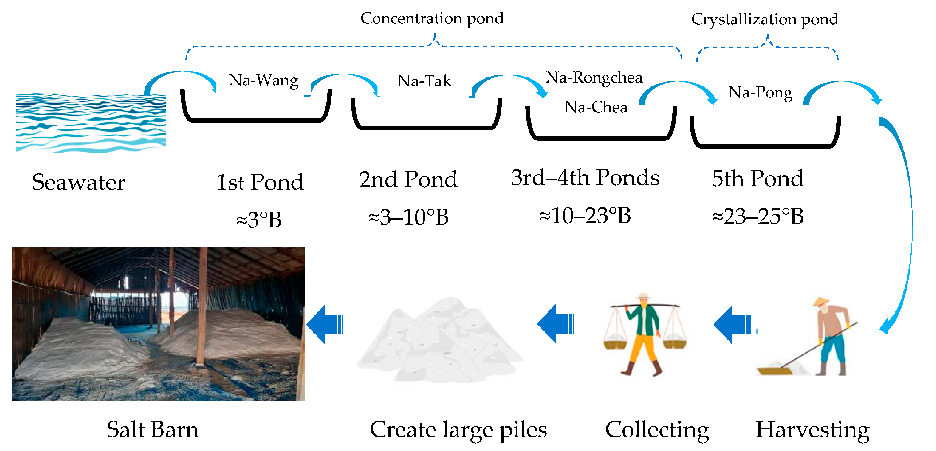
The oldest known technique for producing sea salt is the solar evaporation method. This technique has been used since the discovery of salt crystals in trapped pools of seawater. It is only viable in warm regions where the evaporation rate regularly exceeds the precipitation rate, preferably with consistent prevailing winds. By using this method, sea salt is commonly produced for commercial use by collecting saltwater and storing it in shallow ponds where the sun evaporates most of the water, leaving behind a concentrated brine that crystallizes salt. The salt is then harvested by labor or machine using collecting devices. In general, it is estimated that solar evaporation accounts for about 85% of the total salt production in the world, with the remaining being produced using other methods such as vacuum evaporation and the mining of underground salt deposits [6].

Thailand is a major producer of both sea and rock salt, with sea salt primarily being produced using the traditional solar evaporation system. Thai sea salt production is a traditional and deeply ingrained agricultural practice that is considered one of the oldest occupations of the Thai people. With local wisdom, seawater is collected in shallow ponds and left to evaporate in the sun, resulting in salt crystal precipitation. The salt is then harvested and processed before being cleaned, graded, and packaged for sale. The majority of sea salt production is in central Thailand. Rock salt, on the other hand, is typically mined from underground deposits, with the majority being produced in the north-east.

Both sea salt and rock salt farming are essential parts of the local economies in Thailand, employing many people in the coastal regions. It is also an important cultural practice, with many families and communities having a long salt farming history. Consequently, in 2011, the Thai Cabinet passed a resolution to promote and support sea salt farming as a new form of agriculture and a potential coastal commodity. The resolution aimed to increase the income and quality of life of coastal communities in Thailand by encouraging the production of high-quality sea salt for both domestic and international markets [7,8]. Additionally, the Thai government will soon advocate the registration of Thai sea salt production as a Globally Important Agricultural Heritage System (GIAHS) [8,9].

According to the Office of the Secretary of the Thai Sea Salt Development Board, there were a total of 946 households engaged in sea salt production, cultivating 1595 plots that cover a total area of 7553.65 hectares [9]. Most of the production, accounting for approximately 98% of the total output, was concentrated in three provinces, namely Phetchaburi, Samut Sakhon, and Samut Songkhram. The remaining 2% of production was distributed across four provinces in the central and southern regions, namely Chon Buri, Chanthaburi, Chachoengsao, and Pattani. The Phetchaburi province alone accounted for 32.55% of the total area with 2458.4 hectares. In the 2019/2020 season, the cost of producing sea salt was 0.87 THB per kg and the average yield was 14.78 tons per rai [9]. By 2021, the total cost of producing sea salt was 873.23 THB per ton, with labor costs constituting 63.4% of the total cost [10]. In 2022, sea salt farmers were able to sell their products at an average price of 1275 THB per ton or 1.275 THB per kg. Thailand’s salt production industry faces several challenges, including changing weather patterns, which can affect salt qualities and quantities. In addition, labor shortages have also been a concern, as many young people are no longer interested in working in the salt fields.

Although Thailand has the potential to produce raw salt for domestic consumption, the refined salt industry, and exports, it imported salt for years. The critical issue with the Thai sea salt market in 2019 was imported salt being cheaper than domestically produced salt [11,12]. The relatively cheaper imported salt puts pressure on local producers to lower their prices, which affect their profitability and sustainability. With imports, the domestic sea salt was left unsold and stored in numerous sea salt barns. In response to this issue, the Thai government with the Ministry of Agriculture and Cooperatives implemented policies and programs to support the local salt production industry, including speeding up salt stock release, introducing salt-pledge measures, providing loans for barn renovation and production development, modifying the fair trade rules, and launching marketing and product development initiatives for Thai sea salt [13]. In addition, the Department of Foreign Trade established standards to regulate salt imports and provide support to the local sea salt farmers [14]. However, price competitiveness remains a challenge for Thai salt producers.

Salt demand in Thailand is increasing every year, but the locally produced salt cannot meet this due to several factors such as weather conditions, salt pond locations, and a lack of experience among farmers [8]. In traditional salt production, the salt crystallizes on the ground which results in salt without a clear white hue and contaminates the soil. Outdated technologies, insufficient facilities and operating capital, and inadequate infrastructure and barns are also contributing factors [8]. To ensure the Thai salt industry’s long-term growth and sustainability, increasing both the yield and quality of salt by adopting new technologies, sustainable production practices, and efficient processes that can enhance the salt production process’ effectiveness and efficiency is crucial. One promising way to achieve this is to use High-Density Polyethylene (HDPE) Geomembranes (GMBs) sheets in salt plots [15], which can improve salt productivity and quality.

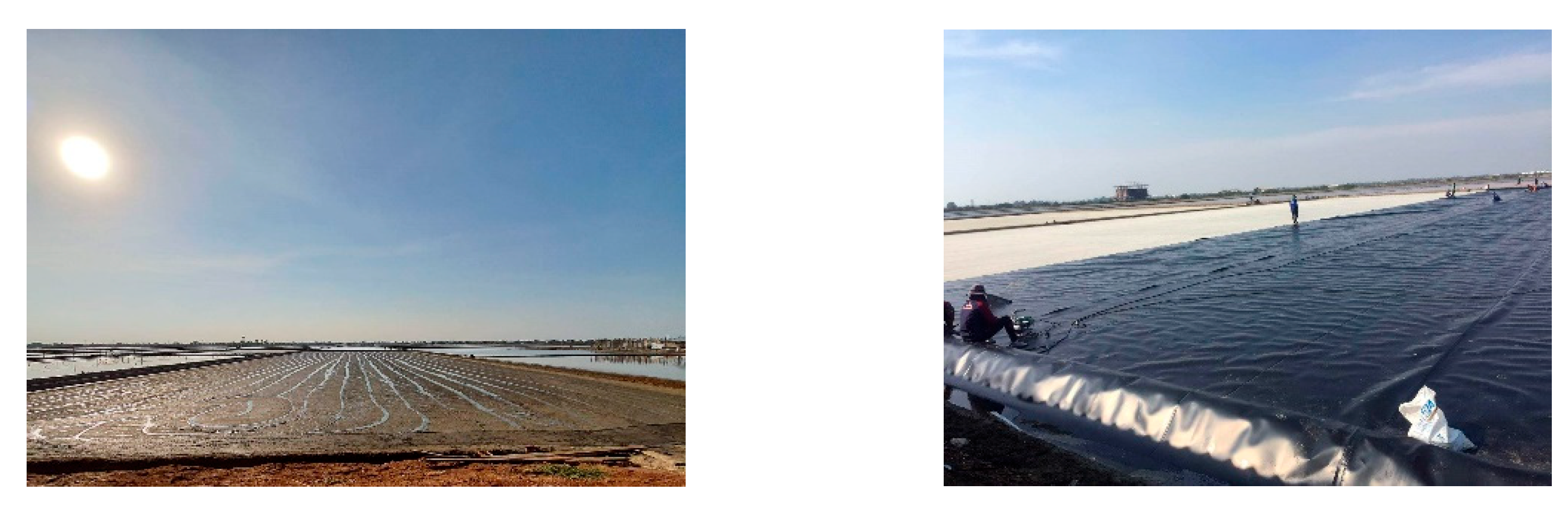
HDPE sheets include a layer of GMBs that are placed on a salt plot’s ground to act as a waterproof barrier between the soil and seawater [16,17]. The use of HDPE GMB sheets can improve the produced sea salt’s quality and quantity to meet market demand and reduce production costs [18]. The results of using HDPE sheets in salt plots have shown that the high-quality white salt yield increased from 20% to 80%, medium-quality salt decreased from 60% to 20%, and low-quality black salt decreased from 20% to 0% [7]. The HDPE sheet’s black color absorbs heat from the sun, which accelerates crystallization and thus shortens the production time. Using HDPE GMB sheets also results in cleaner salt and does not contaminate the soil [15,19,20,21]. The benefits of using HDPE sheets in salt plots include reducing labor, oil–energy, and machine repair costs. Additionally, the salt production cycle can increase from five to seven cycles per year, and the yield per cycle can increase from 24,000 kg/rai to 32,000 kg/rai. Consumers can be assured that the HDPE GMB sheet used in salt fields is created from high-quality, food-grade plastic pellets and has quality certificates to ensure purity. Typically, the use of HDPE GMB in sea salt production is not prevalent, as the traditional solar evaporation method remains the most-used technique due to farmers’ familiarity with the conventional practice and the installation and maintenance costs associated with using geomembranes.

Currently, the Thai Phetchaburi Sea Salt Agricultural Cooperative Ltd. in the Phetchaburi province, Thailand, aims to encourage members to pursue a sustainable salt career and to promote and support using new and appropriate technology, such as HDPE GMB, in sea salt production to improve product quality and meet the Good Agricultural Practices (GAP) for Thai sea salt farming [22]. However, there are no published comparative empirical studies on the efficiency of Thai sea salt production between traditional technology and HDPE GMB. As a result, the cooperative is unable to fully promote supporting and convincing sea salt farmers to adopt HDPE GMB in sea salt production. A few studies on the effectiveness of sea salt production have been undertaken in the past, including Balde (2014) [23] and Dake, M. (2019) [24].

Therefore, the research questions to be addressed are: “What is the efficiency of sea salt production in the Phetchaburi province?” “What factors affect production inefficiency?” “What is the technological difference gap?” This study’s objectives include analyzing and comparing sea salt production efficiency using traditional technology and HDPE GMB technology and examining the factors that contribute to sea salt production inefficiency in the Phetchaburi province.

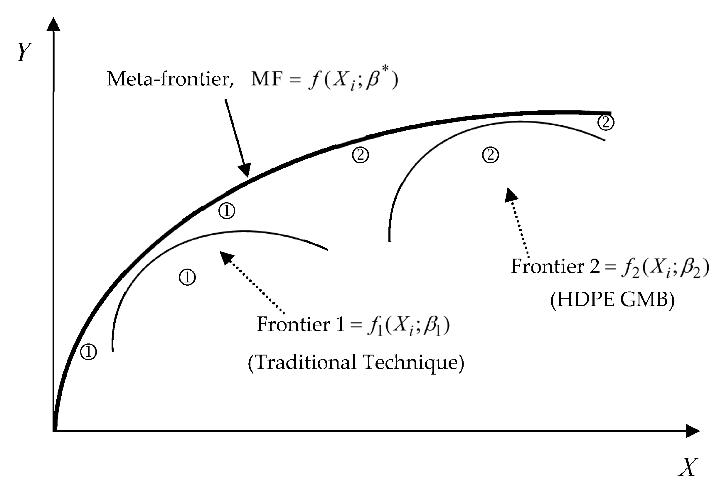
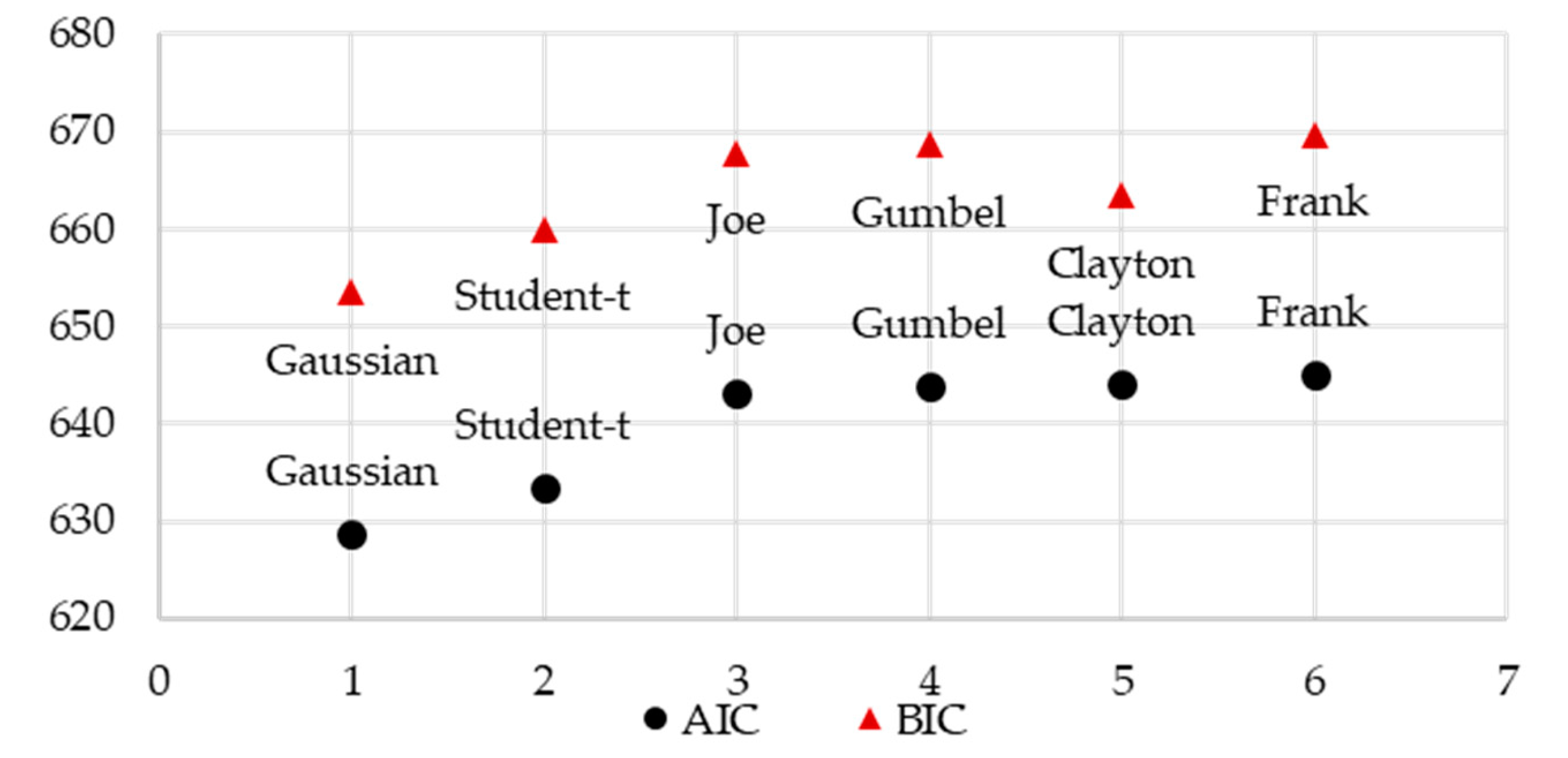
This paper utilizes the copula-based meta-frontier model (CMFM) for this comparison. Moreover, the study explores the dependence structure of two error components using various copula families, such as the Gaussian, Student-t, Clayton, Frank, Gumbel, and Joe families. The best-fit model is selected based on the AIC or BIC criteria. Additionally, the study identifies and examines the determinants of technical inefficiency to provide policy recommendations. This article’s novelty is in its use of a copula-based meta-stochastic frontier analysis to compare the technical efficiency of traditional and HDPE GMB technology of sea salt farmers in Phetchaburi, Thailand. This method provides a more accurate assessment of technical efficiency by considering the interdependence between error components and technology differences. Furthermore, this study contributes to the literature on sea salt farming by identifying the factors affecting technical efficiency and opportunities for improvement. Decision makers can use these findings to enhance efficiency, competitiveness, and profitability in agricultural development, which will ultimately improve the sustainable agricultural system and the livelihood of Thailand’s sea salt farmers. The rest of the paper is organized as follows: Section 2 introduces the econometric model, and Section 3 presents the data collection. The empirical findings are presented in Section 4, and the paper concludes in Section 5.

2. Literature Reviews

2.1. Traditional Sea Salt Production

The traditional Thai sea salt production technology relies on the “Solar Evaporation System”, which is heavily dependent on natural factors such as earth, water, wind, and fire. In particular, salt fields that were previously used for salt farming tend to produce better quality sea salt than the newly developed ones. This is because the soil in these fields has accumulated minerals that facilitate faster sea salt crystallization. The location of salt fields is also important, with the sea or tidal estuaries introducing seawater. To produce high-quality sea salt, the seawater should be free of any contaminants or sediments. Sea salt farmers, therefore, need to ensure that the saltwater canal near their area remains clean to produce salt crystals with good quality, taste, and nutrients. The strength of sea winds blowing towards the shore throughout the sea salt farming season is crucial as it creates ripples on the surface of the water immersed in the field, leading to a water movement system that stirs the water into an equal concentration. This, in turn, facilitates faster and more consistent saline water crystallization. Finally, the constant intensity of sunlight and appropriate heat is essential for the brine surface evaporation in the field, resulting in a very salty brine and large amounts of salt crystallization. These natural factors are fundamental to producing high-quality traditional Thai sea salt, which is a process that remains dependent on the environment and the ingenuity of local salt farmers [8].

Sea salt production in Thailand is based on local wisdom and has been practiced for many years. Traditional methods are still used in salt farming, and Figure 1 shows the process. Salt farming requires an area of at least 30 rai or 4.8 ha and is divided into two parts: concentration ponds and crystallization ponds. The concentration ponds are divided into four sub-concentration ponds, namely Na-Wang, Na-Tak, Na-Rongchea, and Na-Chea, depending on the salinity level. The crystallization pond is called Na-Pong, where salt is produced from salt water with a salinity level of at least 25 degrees Baumé (°B) [22].

The process begins with collecting seawater during high tide and storing it in the first salt pond, Na-Wang. The water is allowed to settle so that the sediments and other contaminants can be removed, leaving behind clear and clean seawater. The seawater is then pushed to the second pond, Na-Tak, using a wind turbine or water pump. The sun’s heat causes the seawater in the ponds to evaporate, and when the salt concentration is appropriate, the seawater is released to the third and fourth ponds, Na-Rongchea and Na-Chea, respectively. When the salt concentration is high enough, the seawater is drained into the last pond, Na-Pong, where it becomes a saturated solution, and salt crystals begin to form on the pond’s surface until they are about three centimeters thick. The salt crystals are then harvested by breaking up the surface of the pond and collecting the salt. The salt is washed, drained, and sun-dried before being stored in a sea salt barn, which is a dry place to prevent moisture and contamination.

Sea salt production in the central region of Thailand, particularly in the Phetchaburi province, typically starts in early November and runs until mid-May of the following year. The salt harvest typically begins in mid-January. The traditional sea salt production process in Thailand is labor-intensive and relies on a combination of traditional knowledge and natural resources. With the concept of a one-output-many-inputs production function in economics, the inputs required for sea salt production in Thailand include labor, land, fuel energy, and technology. Each of these inputs play a critical role in determining the optimal output of the production process.

2.2. HDPE Geomembrane Technology for Sea Salt Production

The HDPE (high-density polyethylene) geomembrane (HDPE GMB) can be a suitable material for lining salt production ponds. There are many advantages of using HDPE GMB technology for sea salt production. First, HDPE GMB is highly resistant to chemicals and corrosion, which helps prevent the contamination of sea salt by outside elements [25]. It also prevents the salt from contaminating the surrounding environment. These cause it to be an ideal material for lining salt production ponds. Second, HDPE GMB provides a durable barrier that can withstand harsh weather conditions and exposure to UV light. This helps to maintain the salt production facility’s integrity and ensure the consistent quality of the sea salt [16]. Third, HDPE GMB can be used to line evaporation ponds or crystallizers, reducing water loss through seepage. This is important in areas where water is scarce or expensive to obtain [26,27]. Fourth, HDPE GMB can be prefabricated offsite, reducing the time and cost required for installation. This allows for faster construction and commissioning of the salt production facility, ultimately increasing efficiency [28]. Finally, HDPE GMB is created from recyclable materials and has a long lifespan. This reduces the environmental impact of the salt production process and helps promote sustainable practices [19].

Using black HDPE GMB as a lining material in sea salt production particularly at the last pond (Figure 2), Na-Pong, has the potential to increase yields. Because of the very low permeability rate, HDPE GMB can effectively prevent water and other substances from seeping through the lining. This can help reduce seawater loss due to seepage, which can increase overall yields. With reduced seepage, less saltwater is needed to produce the same amount of sea salt. This can help farmers conserve water and lower production costs. Using HDPE GMB can help farmers better control the water salinity in the production ponds. This can be achieved by adding or removing water as needed, which can lead to more consistent yields. As a cost-effective option for sea salt manufacturing, HDPE GMB is a strong material with a long service life. Over time, the decreased need for frequent maintenance and repairs may contribute to an increase in yields and profitability. Susanto et al., (2015) [29], and Dwiyitno et al., (2021) [28] found that HDPE GMB could reduce the salt production time from 3 to 2 weeks and increase the yield by preventing pre-crystallized water penetrating the soil.

2.3. Metafrontier Efficiency Model

Production frontier analysis in agriculture is a method of measuring the production efficiency by comparing the actual output $(Y)$ or observed output (such as crop yield) of decision-making units (DMUs) such as firms or enterprises, with the maximum possible output $(Y^{*})$ or frontier output given the current level of inputs $(X_i)$ (such as labor, capital, and fertilized product). Farrell [30] proposed the parametric frontier production function, $Y=f(X_1, X_2, \dots , X_n)$, which is a type of production frontier analysis that estimates the maximum possible output of a given set of inputs using a mathematical function. The production function f can adopt different forms, depending on assumptions about the relationship between the inputs and outputs.

The production function parameters can be estimated using econometric techniques such as ordinary least squares (OLS) regression or maximum likelihood estimation. Once the parameters are estimated, the Farrell production function can be used to calculate the frontier output for any given set of input levels and to measure the technical efficiency of individual farms or enterprises. The distance between this frontier curve and the actual output of a firm is used to measure the inefficiency level and identify areas for improvement in the production process for increasing efficiency and profitability. The technical efficiency (TE) is the ratio between the observed output $(Y)$ and frontier output $(Y^{*})$ at a particular input level or $TE=Y/Y^{*}$. The analysis can be performed using a range of econometrics techniques such as stochastic frontier analysis (SFA) [31,32]. For salt production, Balde (2014), and Dake, M. (2019) applied a stochastic frontier approach for measuring the technical efficiency of small-scale improved salt production in Guinea, and Elmina, Ghana, respectively [23,24].

The stochastic frontier model combines elements of econometric analysis and production theory to estimate the technical efficiency of firms. SFA assumes that there is a stochastic error term in the production process. The stochastic error term is used to estimate the production process’s efficiency by comparing the actual output to the predicted output based on the same level of inputs. SFM is represented by $Y_i=f(X_i:\beta )+{\epsilon }_i$ where ${\epsilon }_i=v_i+u_i$ and $i=1,2,\dots ,n$. v is a random error of the production beyond the producer’s control and $v\sim N(0,{\sigma }_v^2)$. u is a non-negative random variable standing for the inefficiency term and follows the half-normal distribution $u\sim N{(0,{\sigma }_u^2)}^{+}$. The u and v components are independent [33,34,35]. The SFM parameters can be estimated using maximum likelihood estimation. The SFM is applicable to measure and compare the technical efficiency among DMUs if they are under the same technology. However, SFM is not suitable for comparing the technical efficiency of DMUs that operate under different technologies. This is because the SFM assumes that all DMUs are using the same production function and facing the same constraints in terms of the available inputs and technology [36].

The meta-frontier analysis proposed by Hayami and Ruttan (1970) [37] is a method used to compare the efficiency of multiple production frontiers across different technologies. The meta-frontier production model is a commonly used approach in several fields, particularly in agriculture, to compare the efficiency of DMUs operating under different technologies across various agricultural products. This approach has been applied to analyze the efficiency of DMUs in producing different crops, such as grain [38,39,40,41,42,43], chickpeas [44], cocoa [45], organic vegetables [46], and chili [47,48].

The concept of meta-frontier production function assumes that all producers in various production groups have potential access to various production technologies. The analysis then compares the production frontiers of different units using a common “meta-frontier” that represents the best achievable level of production with the most advanced technology among the analyzed units. It is an extension of stochastic frontier analysis (SFA), which measures a firm’s technical efficiency relative to a single frontier that represents the best performance in the industry. Figure 3 illustrates a production function that smoothly encompasses the frontiers of different sea salt production technologies. The difference between the estimated frontier and meta-frontier, which is known as the group-specific frontier, is used to measure the inefficiency level in each technology and is called a production technology gap. Later, Battese and Rao (2002) [49] and O’Donnell et al., (2008) [50] developed a meta-frontier production function model. This can be used to identify the best practices that can be shared across regions or industries to improve efficiency and productivity.

Meta-frontier analysis involves two main steps. The first is to estimate each DMU’s individual frontiers in the sample. This involves estimating a stochastic frontier production function for each DMU, which relates the level of output to the inputs used in production. The second is to construct the meta-frontier, which represents the best level of production that can be achieved with the most advanced technology among the analyzed DMUs. This involves estimating a stochastic frontier production function using the most efficient DMU in the sample [52]. Typically, the efficiency value obtained from the meta-frontier analysis is lower than the efficiency value obtained from the group frontier. To obtain the relevant parameters, a maximum-likelihood estimation can be applied.

However, the independence assumption on u and v for the technical efficiency assessment in STM may not be realistic. To relax such an assumption, the copula function is applied to join two marginal error component distributions and calculate the degree of dependence between the two error components using rank correlation and tail dependence [53,54]. Smith (2008) provided the theory and empirical study and found the dependent structure between u and v in SFM [53]. In agriculture, few studies have employed copula-based SFM. For instance, Wiboonpongse et al., (2015) used the maximum simulated likelihood method to investigate the dependence structure of error components in the SFM and apply it to intercrop coffee production in Northern Thailand [55]. Chaovanapoonphol et al., (2022) modified this model and introduced clustering copula-based stochastic frontier analysis to assess the rice production’s technical efficiency in the upper north of Thailand [56].

Although copula-based stochastic frontier models are useful in assessing technical efficiency, they cannot be used to compare technical efficiency between different groups or samples with varying levels of technology. Therefore, to address this limitation, the copula-based meta-frontier approach is preferred over the copula-based stochastic frontier models. Consequently, we propose utilizing the meta-frontier approach to compare the technical efficiency of different technologies. In agriculture, Liu (2019) proposed using the copula-based meta-frontier (CMFM) approach to evaluate the technical efficiency of the agriculture production of BRIC countries and the United States of America [57].

3. Models

3.1. Meta-Frontier Production Model

According to Battese et al., (2004) [51], the technical efficiency of the ith sea salt farmer for the jth technology of each producer is as follows:

$$Y_{ij}=f(X_{ij},{\beta }_j)e^{v_{ij}-u_{ij}}\equiv e^{X_{ij}{\beta }_j+v_{ij}-u_{ij}},i=1,2,\dots ,N,j=1,2,\dots ,J$$

(1)

where $Y_{ij}$ is the output and $X_{ij}$ is the $k\times 1$ vector of inputs for ith producer, and jth technology, respectively. $f(\cdot )$ is the specified functional forms (Cobb–Douglas production function or Translog production function); ${\beta }_j$ is the $k\times 1$ vector of unknown parameters for the different jth techniques that need to be estimated. The $v_{ij}$ is the noise error term and assumed $v_{ij}\sim N(0,{\sigma }_{vj}^2)$, while $u_{ij}$ is a non-negative random variable and represents the technical inefficiency of the ith firm, assumed as the truncated distribution (at zero) of $u_{ij}\sim N(u_{ij},{\sigma }_{uj}^2)$ [36,51]. For all producers in the industry, the meta-frontier production function model is represented as:

$$Y_i^{*}=f(X_i,{\beta }^{*})\equiv e^{X_i{\beta }^{*}}$$

(2)

that $f(X_{ij},{\beta }^{*})\ge f(X_{ij},{\beta }_j)$ for all $j=1,2$. According to Equation (2) and this condition, the greatest possible output for a given number of input quantities is reflected by the meta-frontier production function. As a result, each technology’s production frontiers are defined as a cover curve beneath the meta-frontier.

Equation (1) can be expressed in terms of the meta frontier function in Equation (2) as follows:

$$Y_i=e^{-U_{ij}}\left[\frac{e^{X_{ij}{\beta }_j}}{e^{X_i{\beta }^{*}}}\right]e^{X_i{\beta }^{*}+V_{ij}}$$

(3)

The technical efficiency relative to the stochastic frontier for the two production systems is provided in the first term on the right-hand side of Equation (3) as follows:

$$T{E}_{ij}=\frac{Y_i}{e^{X_i{\beta }^{*}+V_{ij}}}=e^{-U_{ij}}$$

(4)

According to Battese et al., (2004) [51], the ratio of the observed output to the output from the meta-frontier is the technical efficiency of the ith farm with the meta-frontier and is represented by $T{E}_i^{*}$:

$$T{E}_i^{*}=\frac{Y_i}{e^{X_i{\beta }^{*}+V_{ij}}}$$

(5)

The technical gap ratio (TGR), the second term of Equation (3), is used to measure the technological difference between individual enterprises in groups and the entire industry. Given the observed inputs, TGR is the proportion of the output for the jth frontier production function compared with the potential output from the meta frontier function.

$$TG{R}_{ij}=\frac{e^{X_i{\beta }_j}}{e^{X_i{\beta }^{*}}}$$

(6)

The TGR values vary from zero to one. With the available technology, if TGR is close to 1, the industry’s firms are producing at or near their full potential output.

3.2. Copula-Based Stochastic Frontier Model

Smith (2008) [53] proposed adopting the copula concept to relax the independence assumption between noise (v) and inefficiency (u) and to model this dependence. Sklar (1959) [58] provides Sklar’s theorem that proposed that the joint distribution function between u and v or $F(u,v)$ depends upon the marginal distributions U and V and the unique copula C as follows:

$$F(u,v)=C_{\theta }\left(F_U(u),F_V(v)\right)$$

(7)

where $F_U(u)=\mathrm{Pr}(U\le u)$ and $F_V(v)=\mathrm{Pr}(V\le v)$ are the marginal distribution function of the non-negative random variable and the noise error variable, respectively. Let $w=v-u$ be a composite error in the frontier production function. The joint probability density function of (u, v) is

$$f_{\theta }(w)=f(u,v)=f_U(u)f_V(v)c_{\theta }\left(F_U(u)F_V(v)\right)$$

(8)

where $f_U(u)$ and $f_V(v)$ are the pdf of U and V, respectively. The copula density of $C_{\theta }$ is $c_{\theta }$. Next is the transformation from $f(u,v)$ to $f(u,w)$ is

$$f(u,w)=f_U(u)f_V(w+u)c_{\theta }\left(F_U(u)F_V(w+u)\right)$$

(9)

3.3. Model Specification

In this paper, the three-factor KLE production function was used to model the production process, with Capital (K), Labor (L), and Fuel Energy (E) being the inputs. The stochastic frontier function for all the farms was modeled using the translog form. Specifically, the translog functional form was utilized to describe the production process for the ith farmer on a given farm, and it can be expressed as follows:

$$ln{Y}_i=ln{\beta }_0+{\displaystyle \sum _{j=1}^3{\beta }_{j}ln{X}_{ji}}+\frac{1}{2}{\displaystyle \sum _{j=1}^3{\displaystyle \sum _{k=1}^3{\beta }_{jk}ln{X}_{ji}ln{X}_{ki}}}+v_i-u_i$$

(10)

Thus, the meta-frontier model is specified as:

$$ln{Y}_i^{*}=ln{\beta }_0^{*}+{\displaystyle \sum _{j=1}^3{\beta }_j^{*}ln{X}_{ji}}+\frac{1}{2}{\displaystyle \sum _{j=1}^3{\displaystyle \sum _{k=1}^3{\beta }_{jk}^{*}ln{X}_{ji}ln{X}_{ki}}}+v_i^{*}-u_i^{*}$$

(11)

where $Y_i$ denotes the level of output produced by salt farms (ton). Additionally, the input variables $X_1,X_2$, and $X_3$ correspond to land (rai), labor (number of workers), and fuel energy expenditure (THB/production round), respectively. The error component is assumed to have normal and half-normal distributions for the noise terms and inefficiency terms, respectively. The error component assumed the normal and half-normal distributions for noise terms $V_i$ and inefficiency terms $U_i$, respectively.

The model to analyze the technical inefficiency determinants is expressed as

$$u_{ij}={\delta }_0+{\displaystyle \sum _{m=1}^6{\delta }_m{Z}_{mi}}$$

(12)

where $Z_m$ represents the factors that explain the technical inefficiency. $Z_1$ is the farmer’s age in years. The negative sign means older farmers have more experience and better training services, enabling them to reduce production inefficiencies and losses by gaining more information. However, the positive sign suggests that older farmers may be more conservative and less likely to adopt innovations [59]. $Z_2$ is a dummy variable of land that indicates whether the farmer owns or rents their land. Farmers who own their land are more productive than those who rent [60]. $Z_3$ represents educational attainment. It may have a positive sign, indicating that education has a detrimental influence on a producer’s efficiency, hence increasing inefficiency. This may be because educated farmers have less time for farm labor and may have other employment than agricultural output [61]. However, higher levels of education significantly impact the decision-making and acceptance of innovation by farmers, which may lead to an increase in agricultural yield [62]. $Z_4$ represents a product’s market price. High market prices incentivize farmers to increase production efficiency and accept new technologies [63]. $Z_5$ denotes sex. The negative coefficient for ‘sex’ suggests that male farmers are more likely than their female counterparts to be efficient. This may be because male farmers have more access to institutional support and capital resources [64]. $Z_6$ indicates the distance of the most distant farmland from the farm. The positive coefficient for ‘distance’ indicates the greater the distance, the more efficient the farm is. This may be because certain farmers try to more effectively employ labor and equipment due to the expense of traveling to and from remote regions [65].

3.4. Study Area and Data Collection

The study collected data from registered salt farm farmers who are members of the Thai Sea Salt Agriculture Cooperative Phetchaburi Company Limited, located in three subdistricts: Ban-Laem, Bangkhunsai, and Pakthale in the Ban Laem district of the Phetchaburi province. The study calculated the sample size using the Krejcie and Morgan formula (Equation (13)), which assumes that the population size is known [66]. The formula is as follows:

$$n=\frac{{\chi }^{2}Np(1-p)}{d^2(N-1)+{\chi }^{2}p(1-p)}$$

(13)

where n is the sample size; N is the population size; d represents the required level of precision as a proportion (e.g., 0.05); ${\chi }^2$ is the Chi-square value for one degree of freedom at the desired confidence level, (3.841); and p denotes the population proportion (assumed to be 0.50, as this provides the maximum sample size required for a given level of precision). Out of the population of 317, as determined by Krejcie and Morgan, a sample of 174 was selected. However, in the actual survey, 250 farmers participated, with 195 farmers using traditional technology and 55 farmers using HDPE GMB technology. To gather information on output, input, price data, and exogenous variables, a representative sample of farmers was randomly selected from a list, and interviews were conducted using a meticulously prepared questionnaire. The data on sea salt production were obtained from sea salt farmers during the 2021–2022 production season.

The questionnaire used in the study was divided into three parts. Section A contained questions about the socio-economic characteristics of the sea salt farmers’ respondents, which included their gender, age, education level, salt farm experience, and funding sources. Section B focused on inputs, such as land, labor, fuel energy expenditure, output, and farm management. Section C aimed to identify the problems and obstacles encountered in sea salt farming, such as labor inputs, funding sources, and natural factors.

4. Empirical Results

4.1. Descriptive Statistics

The descriptive statistics gathered from the respondents include information on both the characteristics of the respondents and general details about production and marketing. The data collected on these topics will be separated into two categories for analysis based on the technology used in salt farming: traditional technology and HDPE GMB technology salt farms.

Table 1. Descriptive statistics of respondents.

	Traditional Technology Salt Farms		HDPE GMB Technology Salt Farm
	Number (Persons)	Percentage	Number (Persons)	Percentage
Sex			45
Male	136	69.74		81.82
Female	59	30.26	10	18.18
Age range
Less than 31 years old	1	0.51	0	0.00
31–45 years old	48	24.62	19	34.55
46–60 years old	87	44.62	23	41.82
Over 61 years old	59	30.26	13	23.64
Education level
Primary	111	56.92	23	41.82
Middle school	63	32.31	11	20.00
High school	14	7.18	13	23.64
Bachelor’s degree	4	2.05	5	9.09
Postgraduate	3	1.54	3	5.45
Salt farming experience
Less than 11 years	23	0.12	8	0.15
11–20 years	59	0.30	18	0.33
21–30 years	70	0.36	13	0.24
Distance from home to farm
0–5 km	139	71.28	20	36.36
6–10 km	32	16.41	33	60.00
11–15 km	24	12.31	2	3.64

Source: From the questionnaire.

displays the descriptive statistics of salt farm farmers, focusing on their gender, age, education level, experience, and distance from their home to the salt farm. The data were further categorized based on the technology employed in salt farming, and it was observed that most were male. A review of the age data of the farmers who participated in the survey showed that the average age was 53.11 years. On further analysis, it was observed that the average age of the traditional technology salt farmers was 51.60 years, while the HDPE GMB technology salt farmers had a slightly higher average age of 53.52 years. Examining the data based on age groups revealed that many farmers fall in the age bracket of 46–60 years. This indicates that a significant portion of salt farmers in the Phetchaburi province are advanced in age, with a substantial proportion being elderly. Conversely, the number of farmers aged 31 and below is relatively low. This demographic pattern may have implications for the future of salt farming in the region.

Based on the collected data on farmer’s education levels, it was observed that most of the salt farmers had only completed primary school. Additionally, most of the traditional technology salt farmers had 21–30 years of experience in salt farming, whereas the HDPE GMB technology salt farmers had 11–20 years of experience. The findings further indicate that more than 50% of all respondents had over 20 years of experience in salt farming, which is in line with the high average age of the farmers mentioned earlier. In addition, most of the traditional technology salt farmers had their farms situated close to their homes, with distances less than 5 km. Conversely, the HDPE GMB technology salt farmers had a higher distance from their homes to the farms, located at a distance of 6–10 km.

Table 2. Descriptive statistics of farm input variable utilization by group.

Variable	Traditional Technology				HDPE GMB Technology
	Max	Min	Mean	SD	Max	Min	Mean	SD
Land size (Rai)	200	4	48.57	31.89	320	3	89.37	79.25
Number of workers used (person)	15	2	5.80	2.73	18	2	6.86	3.85
Fuel expenses/year (thousand THB)	178.80	43.70	83.66	25.80	286.6	44	104.30	56.44

Source: From the questionnaire.

, which presents the descriptive statistics of farm input variable utilization by technology, indicates that sea salt farming utilizing HDPE GMB technology had a higher average farm area than those using traditional technology. This trend was also reflected in the data concerning labor and fuel costs. However, it is important to note that the standard deviation for this factor was higher among the salt farmers using HDPE GMB technology than those using traditional technology.

Figure 4 displays the salt yield data, which reveal that the traditional technology salt farmers achieved an average yield of 8.88 wagons per rai per year or 13.32 tons per rai per year (one wagon of salt equivalent to 1.5 tons) in the 2021/2022 production year. The highest and lowest yields recorded were 12.50 and five wagons per rai per year, respectively. In comparison, the HDPE GMB technology salt farms had a higher yield, with an average of 11.98 wagons per rai per year or 17.97 tons per rai per year. The highest and lowest yields were 25.00 and 10.00 wagons per rai per year, respectively. This finding is consistent with previous studies on sea salt production using HDPE GMB technology in Indonesia, such as Suhendra (2016) [28], Sulistyaningsih and Alighiri (2018) [19], and Susanto et al., (2015) [29]. The variation in salt production from the traditional technology salt farms was lower than that of the HDPE GMB technology salt farms.

4.2. Test of Model

To assess the specified meta-frontier model’s suitability, the hypotheses are investigated. These hypotheses aim to evaluate the model’s adequacy and determine whether it can effectively explain the variations in technical efficiency between different groups. The relevance of exogenous variables to explain inefficiency was also assessed using this testing process. The first test $H_0:{\beta }_4={\beta }_5=....={\beta }_9=0$ involves examining whether the coefficients of the second-order variable in the translog model, (β_ij) are equal to zero. If the result indicates that the coefficients are zero, then the Cobb–Douglas function can be considered a statistically valid representation of the data. The second test, $H_0:\gamma ={\delta }_0={\delta }_1=\dots ={\delta }_6=0$, involves testing whether inefficiency effects are present in the models at any level. If the result shows that inefficiency effects are absent from the models at all levels, then the model can be considered accurate in capturing the variations in technical efficiency between different groups. The third test, $H_0:f(X_{ki};{\beta }_k)=f(X_{ji};{\beta }_j)$, involves assessing whether there is a significant difference between the traditional and HDPE GMB technology. A non-significant result would suggest that there is no need for specifying the meta-frontier production model.

The generalized likelihood–ratio statistic was used to test these hypotheses, which involved calculating the $LR=–2\left[\ln \left(L(H_0)\right)–\ln \left(L(H_1)\right)\right]$, where $L(H_0)$ and $L(H_1)$ represented the likelihood function of the null and alternative hypotheses, respectively. Coelli (1995) suggests that all critical values can be derived from the corresponding Chi-square distribution [67]. However, in cases where the hypothesis test involves γ = 0, the mixed Chi-square distribution is required due to the asymptotic distribution (Kodde and Palm 1986) [68].

The tested hypotheses’ results are presented in

Table 3. Results of the hypothesis testing with LR-test.

Null Hypothesis	Likelihood Ratio Test (LR-Test)		Decision
$H_0:{\beta }_4={\beta }_5=....={\beta }_9=0$	Traditional Technology	16.013 ***	Rejected $H_0$
	HDPE GMB Technology	13.241 ***	Rejected $H_0$
$H_0:\gamma ={\delta }_0={\delta }_1=\dots ={\delta }_6=0$	Traditional Technology	15.774 ***	Rejected $H_0$
	HDPE GMB Technology	14.216 ***	Rejected $H_0$
$H_0:f(X_{ki};{\beta }_k)=f(X_{ji};{\beta }_j)$	Pools	41.23 ***	Rejected $H_0$

Source: Own Calculation. Note: *** represents significance at 1% level.

. The initial hypothesis aimed to assess the suitability of the Cobb–Douglas or translog model for sea salt production using traditional and HDPE GMB technology. Under the null hypothesis that the translog model was not appropriate for traditional technology salt production and HDPE GMB technology, we rejected the null hypothesis at a significant level of 1%. The second hypothesis aimed to investigate the presence of technical inefficiency effects in sea salt production using traditional and HDPE GMB technology. The high LR-test value indicated rejecting the null hypothesis, at a 1% significant level, implying that inefficiency effects were absent in the model. Therefore, the stochastic production function frontier was the most suitable approach. Lastly, the objective was to determine if there are any differences or similarities between the traditional and HDPE GMB technology in sea salt production. At a 1% significant level, we rejected the null hypothesis, indicating that there is a significant difference between traditional technology and HDPE GMB technology, meaning the meta-frontier model was the appropriate estimation method for this study, and that the efficiency comparison between these two production systems should be based on the meta-frontier instead of the pooled stochastic frontier. These findings are in line with previous studies on agricultural production using various technologies, including Mariko et al., (2019) [42], Onumah et al., (2013) [45], and Krasachat (2023) [48].

Table 4. Estimated parameters and standard errors for the meta-frontier model based on six different copula families.

Variable	Copulas
	Gaussian		Student-t		Clayton		Gumbel		Frank		Joe
	Coef.	S.E.	Coef.	S.E.	Coef.	S.E.	Coef.	S.E.	Coef.	S.E.	Coef.	S.E.
Constant	−1.863	0.428	−1.460	0.276	−0.755	1.774	−2.567	1.911	−0.604	0.589	−2.993	0.595
lnland	3.118	0.867	4.960	0.379	3.185	3.947	3.729	3.818	4.069	4.558	3.495	3.877
lnlabor	−1.783	0.710	0.906	0.302	−1.732	3.028	−0.780	2.895	−1.211	3.129	−0.668	2.880
lnenergy	−4.672	0.570	−2.644	0.283	−4.152	3.183	−3.072	2.993	−3.467	3.432	−2.919	3.003
½(lncapital)2	−0.314	0.092	−0.458	0.041	−0.404	0.363	−0.405	0.365	−0.477	0.412	−0.371	0.374
½(lnlabor)2	1.052	0.065	0.937	0.043	0.945	0.356	0.835	0.342	0.876	0.375	0.810	0.341
½(lnenergy)2	0.064	0.059	−0.287	0.031	0.016	0.262	−0.084	0.245	−0.021	0.261	−0.104	0.240
½(lncapital × lnlabor)	−0.430	0.143	−0.973	0.070	−0.390	0.582	−0.506	0.573	−0.478	0.611	−0.488	0.579
½(lncapital × lnenergy)	0.188	0.125	0.217	0.077	0.226	0.754	0.056	0.706	0.059	0.860	0.070	0.716
½(lnlabor × lnenergy)	0.463	0.129	0.173	0.063	0.444	0.544	0.345	0.528	0.390	0.546	0.331	0.521
Log-likelihood	−304.338		−305.893		−311.992		−311.959		−312.469		−311.518
AIC	628.695		633.347		644.005		643.938		644.958		643.055
BIC	653.494		660.052		663.537		668.736		669.756		667.854

Source: Own calculation.

shows the estimated parameters and standard errors of the meta-frontier model based on six different copula families for sea salt production, namely the Gaussian, Student-t, Clayton, Frank, Gumbel, and Joe families. The AIC and BIC values of six different copula families of the meta-frontier are illustrated in Figure 5. The best model for meta-frontier sea salt production uses Gaussian copulas due to its minimal AIC and BIC values compared to the other five different copula families.

4.3. Estimated Model

Table 5. Parameter estimates of the Gaussian copula-based meta-frontier production models.

Variables	Traditional Technology		HDPE GMB Technology		Pools (Meta)
	Parameters	p-Value	Parameters	p-Value	Parameters	p-Value
Constant	25.330 ***	0.000	3.286 ***	0.000	−1.333 ***	0.000
lnland	−2.068 **	0.014	2.021 *	0.087	2.231 **	0.021
lnlabor	−5.960 *	0.048	6.381 *	0.091	−1.276 **	0.033
lnenergy	−4.645 *	0.074	−2.779	0.312	−3.343 ***	0.000
½(lncapital)2	−0.198 **	0.032	0.395 **	0.044	−0.225 **	0.047
½(lnlabor)2	0.898 **	0.044	−0.466	0.211	0.753 *	0.063
½(lnenergy)2	0.253 *	0.512	−0.366 **	0.049	0.046 *	0.067
½(lncapital × lnlabor)	0.712	0.778	−0.951 *	0.088	−0.308	0.313
½(lncapital × lnenergy)	0.778 *	0.055	−0.103	0.108	0.134 *	0.087
½(lnlabor × lnenergy)	0.759 *	0.078	−0.744 *	0.041	0.331 **	0.000
${\sigma }_u$	0.501	0.314	1.125 **	0.033	1.607	0.128
${\sigma }_v$	0.903	0.233	0.932 *	0.082	2.082	0.164
$\theta$	13.264 ***	0.000	5.984	0.122	-	-
${\sigma }^2$	0.867 **	0.041	1.736 *	0.058	-	-
$\rho$	0.311 *	0.087	1.044 **	0.047	-	-
$\lambda$	0.681	0.145	1.485 *	0.051	-	-
$\gamma$	0.289 *	0.000	0.729 *	0.213	-	-
Log-likelihood	−32.115		−41.213		−234.331
LR ratio test	12.314		14.211		41.234
Mean efficiency	0.578		0.674		0.612

Source: Own calculation. Note: ***, **, and * represents significance at 1%, 5%, and 10% levels, respectively.

displays the estimated parameters for the translog meta-frontier production of sea salt, utilizing Gaussian copula-based estimates. The findings revealed that the technical efficiency of HDPE GMB technology was higher than that of traditional technology, with values of 0.674 and 0.578, respectively. The findings align with those of Suhendra, A. (2016) [28], which demonstrated that using HDPE geomembranes to line a larger area of salt evaporation ponds leads to increased salt yields. Therefore, utilizing HDPE geomembranes in salt evaporation ponds provides several advantages and favorable outcomes for improving salt yields.

The β_i coefficients in the translog model represent the output elasticity of the ith input (lnland, lnlabor, and lnenergy); notable differences were observed between the traditional technology and HDPE GMB technology. For traditional technology, a 1% increase in the total area, total labor applied, and total energy expenditure used for sea salt production leads to a decrease in the harvested sea salt quantity by 2.068%, 5.960%, and 4.645%, respectively. In contrast, in the HDPE GMB technology, the harvested sea salt quantity increased by 2.021% and 6.381% but decreased by 2.779%, if each input increased by 1%, respectively.

Findings from the field survey revealed that HDPE GMB technology sea salt farmers tend to have larger farms than traditional sea salt farmers. With HDPE GMB production technology yielding more sea salt than traditional production, having more land can increase productivity. This finding is supported by various other agricultural studies, which show that increasing land size can lead to a corresponding increase in agricultural yield such as Geffersa et al., 2022 [69]; Tweneboah Kodua et al., 2022 [70]; and Scholz and Abdulai, 2022 [71]. However, field surveys revealed that most traditional sea salt farmers are smallholders who allocate an excessive amount of land for saline water storage complementing with the overuse of other inputs, which could reduce the sea salt yield. This overuse may be due to smallholders using more inputs compared to larger farmers who use fewer inputs. This finding is consistent with a study conducted by Begum et al., 2015 [72]. Therefore, reducing water storage land use has the potential to increase sea salt yield.

The relationship between the labor factor and production efficiency varied between traditional salt production technology and HDPE GMB technology. The labor factor in traditional technology salt production had an inverse relationship with production efficiency, with a coefficient of 5.960, whereas the labor factor in HDPE GMB technology sea salt production had a positive relationship with the production efficiency, with a coefficient of 6.381. Salt farming is a labor-intensive occupation that requires significant manual labor throughout the production process. In traditional technology salt farming, there are various labor-intensive activities, particularly scraping off all residual salt from the soil surface and managing the water circulation in sea salt plots, which can require a week to complete, especially in cases where there is a shortage of labor. If left untreated, this residual salt can decrease the subsequent salt yield and quality. Therefore, in the traditional production system, the number of workers is inversely related to the amount of sea salt production. However, in the HDPE GMB technology system, water management activities are prioritized, and less manual labor is required for land preparation in salt fields. This reduces the need for heavy labor, leading to higher production efficiency compared to traditional technology. Therefore, the use of labor factors in the HDPE GMB technology production system has a positive correlation with sea salt production, which is consistent with the previous studies of Obianefo et al., 2021 [43].

The energy variable was found to have a significant impact on the specific production efficiency of traditional technology salt farming, with a coefficient of 4.645 in the opposite direction. In traditional salt farming, fuel energy is used for rolling salt fields and pumping water in production areas. This indicates that reducing fuel consumption may increase production efficiency for traditional technology salt farming systems. Therefore, it is essential to adopt sustainable practices that reduce fuel consumption and production costs to optimize salt production in traditional technology salt farming.

4.4. Technology Gap Ratios

Table 6. Summary statistics for the technical efficiencies obtained the meta-frontier models for sea salt farm production.

	Min	Max	Mean	Std.
Technical efficiency (meta-frontier)
Traditional Technology	0.147	0.623	0.578	0.159
HDPE GMB Technology	0.237	0.862	0.674	0.175
Pools	0.147	0.862	0.612	0.214
Technology gap ratios
Traditional Technology	0.514	0.941	0.698	0.122
HDPE GMB Technology	0.511	0.978	0.771	0.122

Source: Calculation.

displays the findings of the meta-frontier analysis, which estimated the average technical efficiency of salt farms utilizing traditional technology and HDPE GMB technology to be 0.578 and 0.674, respectively, concerning the meta-frontier. However, to achieve the maximum potential performance in their sea salt production systems, sea salt farmers must consider the difference between their current performance level and the desired level of technical efficiency.

Figure 6 demonstrates the technical efficiency distribution of salt farms: the mean technology gap ratio for traditional technology salt farms was 0.698, while it was 0.771 for HDPE GMB technology farms. This indicates that, on average, producers using the HDPE GMB technology system are more technically efficient than those employing traditional technology. These results suggest that if salt farms using traditional technology were to achieve technical efficiency, they could increase their output by 30.20% by closing the gap, whereas HDPE GMB technology farms could increase their output by 22.90% by performing the same. Figure 7 illustrates the technical performance of traditional and HDPE GMB technology in sea salt farming production. Therefore, these findings highlight the need for salt farmers to adopt efficient technologies and practices to optimize their production efficiency and output.

4.5. Determinants of Technical Inefficiency

Table 7. Parameter estimates of the inefficiency model.

Variable	Traditional Technology		HDPE GMB Technology
	Coefficient	p-Value	Coefficient	p-Value
Constant	0.968 ***	0.000	0.854 ***	0.000
Age	−0.231	0.123	0.122	0.114
Land	0.127 **	0.041	0.236 *	0.073
Education	0.012	0.223	−0.014	0.169
Market price	0.231 *	0.078	0.211	0.254
Sex	−0.314 *	0.081	−0.212 *	0.091
Experience	0.223 *	0.064	0.218 **	0.021
Distance	0.274	0.176	−0.122	0.201

Source: Own calculation. Note: ***, **, and * represents significance at 1%, 5%, and 10% levels, respectively.

displays the technical inefficiency model that reveals the impact of different factors on the inefficiency levels. The land variable significantly affected both traditional and HDPE GMB salt farmers with significance levels of 5% and 10%, respectively. During field visits, researchers observed that salt farmers who own farms tend to have more land and can independently manage their salt farms without hiring workers. However, having a large amount of land and being a sole farmer can lead to the inadequate supervision and management of production activities, resulting in higher production inefficiencies. The positive coefficient for land ownership contradicts the idea that land ownership incentivizes farmers to improve productivity. This finding is supported by other studies, such as Donkor and Owusu (2014) [73], Dube et al., (2018) [74], and Deininger et al., (2003) [75], who suggest that limitations in land ownership, such as owning large and remote lands with unsuitable plot characteristics, may restrict farmers’ access to land and affect technical inefficiency.

The study revealed that the inefficiency of both traditional technology salt farmers and HDPE GMB technology salt farmers were negatively and significantly affected by gender at a 10% level. Female farmers reported facing more difficulties than their male counterparts in using traditional water pumps, as the salt field is divided into multiple parts. This can lead to overusing production factors and higher fuel costs, resulting in production inefficiencies. Female farmers may also encounter other factors that may impact technical efficiencies, such as not attending production knowledge meetings due to household chores. On the other hand, male farmers may have easy access to credit since they own most of the property in the household, which can be used as collateral to access credit. Similar results were obtained by Binam et al., (2008) [76], Onumah et al., (2010) [77], and Onumah et al., (2013) [45].

The study discovered that the experience of salt farmers positively affected the inefficiency levels of both traditional and HDPE GMB technology farmers. Even though farmers with significant experience in agriculture had an advantage when managing water in salt fields and predicting the harvest date, those with less experience were found to have lower inefficiency levels. These results align with previous studies by Sienso et al., (2014) [78] and Tweneboah Kodua et al., (2022) [70], which showed that older farmers with many years of experience tend to be less efficient compared to younger farmers who are more willing to adopt new technologies and techniques. Experienced farmers may be hesitant to change their traditional farming practices.

The market price variable was positive for HDPE GMB technology and significantly positive for traditional technology. The primary issue in agriculture that farmers faced was low selling prices (Kwawu et al., 2022 [79]). Particularly during the field survey period, there was an excess supply of traditional sea salt products, causing sea salt price fluctuations to drop below the production cost. This caused farmers to neglect production by slowing down harvesting, leading to inefficiencies.

According to the study, age, education, and distance between the farmer’s house and the salt farm did not significantly affect the inefficiency levels. The results of the estimated variables revealed that the age of farmers had a negative and insignificant impact on traditional technology but a positive impact on HDPE GMB technology. The negative sign suggested that older farmers were less efficient than younger ones, possibly due to the latter’s increased energy and technical proficiency, while the positive sign indicated the opposite, as supported by the findings of Mehmood et al., (2017) [80] and Chiona et al., (2014) [81].

The study found that the education coefficient was not significant for both traditional and HDPE GMB technology salt farmers, but education’s impact was negative for traditional technology and positive for HDPE GMB technology on technical efficiency. This suggests that education can play a key role in improving production technology, as the HDPE GMB technology group showed higher efficiency levels than the traditional technology group, which is supported by Ali et al., (2019) [82].

The study found that the distance between the sea salt farm and the farmer’s home has a significant positive impact on inefficiency levels for traditional sea salt farmers. This is particularly relevant given that most farmers using traditional technology are older. Longer distances between the home and farm increase costs and management efforts, leading to reduced production efficiency. In contrast, most farmers using HDPE technology are commercially oriented, as it saves time, reduces labor employment, and leads to more efficient management, resulting in less inefficiency. These findings align with previous studies conducted by Olarinde (2011) [83] and Miriti (2021) [84].

5. Conclusions

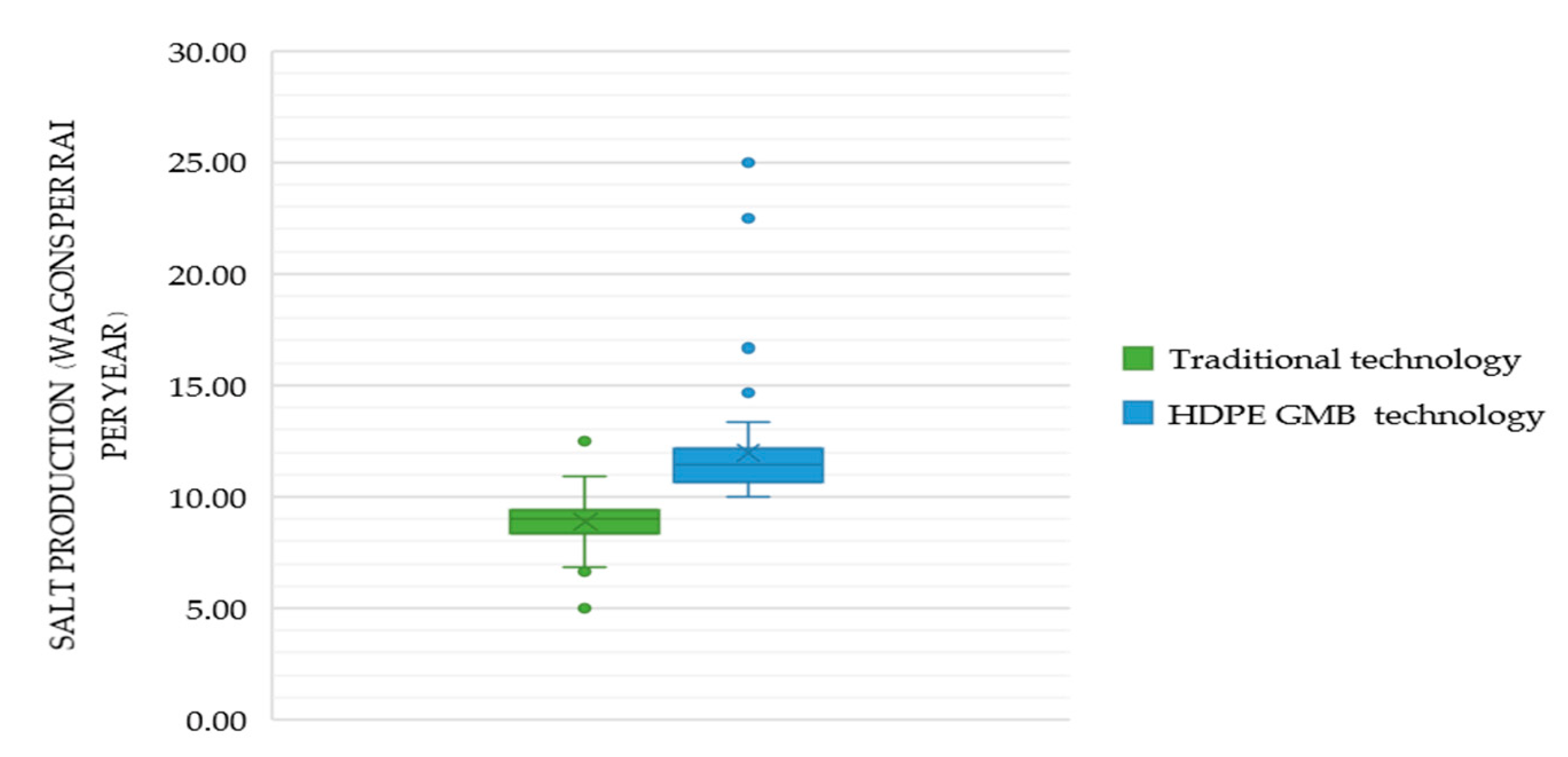
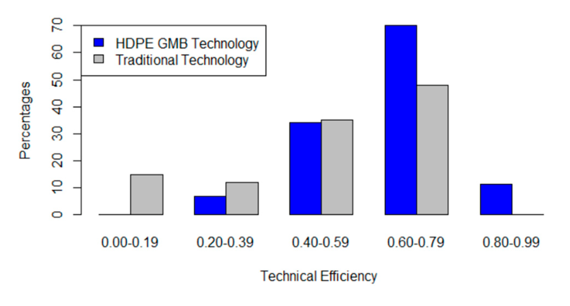
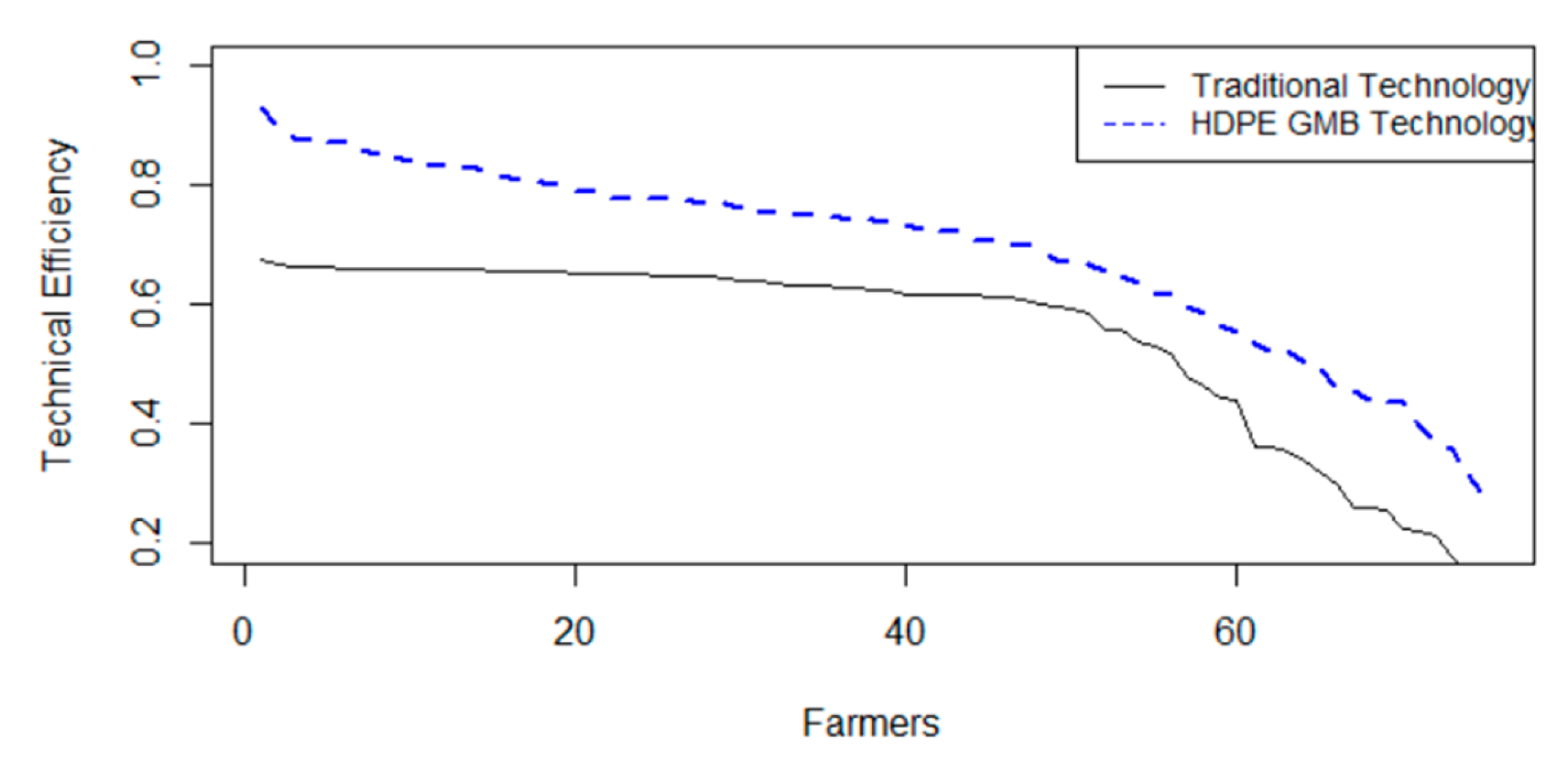
This study analyzed and compared traditional and HDPE GMB technology in sea salt production in the Phetchaburi province using a copula-based meta-stochastic frontier technique with a sample size of 250 farmers. Various copula families were employed to analyze the dependence structure of the two error components. The Gaussian copula-based meta-frontier model with a translog production function was the best fit, suggesting that the assumption of independence between the two error components in the stochastic frontier model can be relaxed. Land, labor, and fuel energy were the most significant input variables. The study found that producers operating under the HDPE GMB technology system are more technically efficient than those operating under traditional technology. The study identified the driving factors of technical inefficiency, which included land, market, sex, and experience for traditional technology production and land, sex, and experience for HDPE GMB production technology. The factors affecting technical inefficiency for traditional technology production were land, market, sex, and experience, while, for HDPE GMB production technology, the factors were land, sex, and experience.

To increase HDPE GMB technology adoption in salt farming, relevant public and private sector agencies should promote greater access to this technology through government subsidies with low-interest conversion. Additionally, educating and demonstrating salt farming techniques with HDPE technology can help increase farmers’ acceptance of this technology, leading to improved salt quality, yields, and prices and greater production efficiency through reduced labor and fuel usage. Although HDPE GMB technology has been successful in improving sea salt production, traditional salt farming practices continue to be prevalent in many areas. To overcome weather-related yield failures, farmers should receive training to become more resilient and adaptable to changing conditions. In addition, promoting traditional salt farming practices for inclusion in the Globally Important Agricultural Heritage Systems (GIAHS) can help increase their value and recognition, highlighting the importance of local expertise and potentially attracting more consumer interest and demand.

6. Limitations and Future Recommendations

This study has some limitations to consider. Firstly, the empirical model used in this study could be biased due to the possibility of an omitted variables problem. Secondly, the limited sample size could affect the model estimation’s accuracy. Thirdly, the data collection period coincided with the COVID-19 pandemic and the harvest season in 2022, which could have increased the difficulty of collecting data through questionnaires. Lastly, corresponding with respondents in the targeted areas may have been challenging due to the use of local languages. Future studies should also consider the cost of HDPE GMB and apply cost-oriented and profit-oriented approaches to provide a more comprehensive analysis of the sea salt production process. To conduct a comprehensive sustainability study in sea salt production, future studies should collect panel data to analyze the changes in production efficiency and sustainability over time and identify trends and patterns. Modeling panel data can also identify factors that contribute to sustainability and efficiency, informing targeted interventions and policy changes to promote sustainable practices.

References

1. Shahbandeh, M. Salt Industry Worldwide—Statistics & Facts. 2022. Available online: https://www.statista.com/topics/5939/salt-industry-worldwide/ (accessed on 20 October 2022).
2. U.S. Geological Survey. Mineral Commodity Summaries: Salt Statistics and Information. Available online: https://pubs.usgs.gov/periodicals/mcs2023/mcs2023-salt.pdf (accessed on 20 February 2023).
3. United Nations Comtrade Database. HS 250100. Available online: https://comtradeplus.un.org/ (accessed on 20 October 2022).
4. ReportLinker. Industrial Salts Market by Source, Manufacturing Process, and Application: Global Opportunity Analysis and Industry Forecast, 2021–2030. Available online: https://www.reportlinker.com/p06193528/Industrial-Salts-Market-by-Source-Manufacturing-Process-and-Application-Global-Opportunity-Analysis-and-Industry-Forecast-.html (accessed on 20 December 2022).
5. Freedonia Group. Global Salt—Industry Reports, Global. Available online: https://www.freedoniagroup.com/industry-study/global-salt-w1003.htm (accessed on 20 December 2022).
6. O’Brien, T.F.; Bommaraju, T.V.; Hine, F. Handbook of Chlor-Alkali Technology: Volume I: Fundamentals, 2nd ed.; Springer: New York, NY, USA, 2005. [Google Scholar]
7. Department of Agriculture Extension. Registration of Farmers for Sea Salt Farming. Available online: http://www.edoae.doae.go.th/salt_farm_260911.pdf (accessed on 20 December 2022).
8. Phetchaburi Provincial Agriculture and Cooperatives Office. Sea Salt Agricultural Development Plan, Phetchaburi Province, Year 2017. Available online: https://www.phetchaburi.go.th/phet2/CODE/files/1502763242_salt.pdf (accessed on 20 December 2022).
9. Office of the Secretary of the Thai Sea Salt Development Board. The Thai Sea Salt Development Committee Report, Fiscal Year 25. Available online: https://drive.google.com/file/d/1AWoj02Yx0Zr4W_d03Hq687r1dI4FbpGI/view (accessed on 20 February 2023).
10. Office of the Secretary of the Thai Sea Salt Development Board. Cost of Salt Production. Available online: https://thaiseasalt.doae.go.th/%e0%b8%95%e0%b9%89%e0%b8%99%e0%b8%97%e0%b8%b8%e0%b8%99%e0%b8%81%e0%b8%b2%e0%b8%a3%e0%b8%9c%e0%b8%a5%e0%b8%b4%e0%b8%95%e0%b9%80%e0%b8%81%e0%b8%a5%e0%b8%b7%e0%b8%ad (accessed on 20 December 2022).
11. Ministry of Commerce. Import of Thailand Classified by Commodity: Import of Thailand Classified by Commodity. Available online: https://tradereport.moc.go.th/Report/ReportEng.aspx?Report=HarmonizeCommodity&Lang=Eng&ImExType=1&Option=1 (accessed on 20 December 2022).
12. Siamrath. The Ministry of Agriculture and Cooperatives Has Set 5 Measures to Solve the Sea Salt Price Crisis and Accelerate the Release of Overflowing 25,000-Ton Salt Warehouses. Available online: https://siamrath.co.th/n/120257 (accessed on 20 December 2022).
13. Ministry of Agriculture and Cooperative. Ministry of Agriculture Submits Decree Interpreting Salt as an Agricultural Product Ready to Support the Production System—Market—Standards after the Sea Salt Farmers in 3 Provinces Complained about the Problem of Continually Declining Salt Prices. Available online: https://www.moac.go.th/news-preview-401991791402 (accessed on 20 December 2022).
14. Department of Foreign Trade. Announcement of the Ministry of Commerce Re: Prescribing Salt as a Commodity that Requires a Certificate and Must Comply with the Coordination Measures for Importation into the Kingdom. Available online: https://www.dft.go.th/th-th/Detail-Law/ArticleId/19348/19348 (accessed on 20 December 2022).
15. Apriani, M.; Hadi, W.; Masduqi, A. Physicochemical properties of sea water and bittern in Indonesia: Quality improvement and potential resources utilization for marine environmental sustainability. J. Ecol. Eng. 2018, 19, 1–10. [Google Scholar] [CrossRef] [Green Version]
16. Guntur, G.; Jaziri, A.A.; Prihanto, A.A.; Arisandi, D.M.; Kurniawan, A. Development of salt production technology using prism greenhouse method. In Proceedings of the IOP Conference Series: Earth and Environmental Science, Jakarta, Indonesia, 9–10 August 2017; Volume 106, p. 012082. [Google Scholar]
17. Abdelaal, F.B.; Morsy, M.S.; Rowe, R.K. Long-term performance of a HDPE geomembrane stabilized with HALS in chlorinated water. Geotext. Geomembr. 2019, 47, 815–830. [Google Scholar] [CrossRef]
18. Ramly, Z.A.; Ahmad, N.; Juhaseng, N.A. Geomembrane Filter Thread Technique’s Potential to Increase Salt Production in Jeneponto Regency. Indones. J. Environ. Manag. Sustain. 2022, 6, 76–81. [Google Scholar] [CrossRef]
19. Sulistyaningsih, T.; Alighiri, D. Quality monitoring of salt produced in Indonesia through seawater evaporation on HDPE geomembrane lined ponds. In Proceedings of the International Conference on Mathematics, Science and Education 2017, Semarang, Indonesia, 18–19 September 2017; IOP Publishing: Bristol, UK, 2018; Volume 983, p. 012166. [Google Scholar]
20. Lestari, W.; Rahmayani, R.F.I.; Evalina, A.; Saputra, M.; Suryani, A.I. Technology development of salt products using geomembrane thread filter technology in Kajhu Village Baitussalam, Aceh Besar. In Proceedings of the 2nd International Conference on Advance & Scientific Innovation, Medan, Indonesia, 19–20 July 2019; IOP Publishing: Bristol, UK, 2018; Volume 1424, p. 012050. [Google Scholar]
21. Tuomela, A.; Ronkanen, A.K.; Rossi, P.M.; Rauhala, A.; Haapasalo, H.; Kujala, K. Using geomembrane liners to reduce seepage through the base of tailings ponds—A review and a framework for design guidelines. Geosciences 2021, 11, 93. [Google Scholar] [CrossRef]
22. National Bureau of Agricultural Commodity and Food Standards. Good Agricultural Practices for Sea Salt Farming. Available online: https://www.acfs.go.th/files/files/commodity-standard/20191223104522_900401.pdf (accessed on 20 December 2022).
23. Balde, B.S.; Kobayashi, H.; Nohmi, M.; Ishida, A.; Matsumura, I.; Esham, M.; Tolno, E.A. Stochastic Frontier Approach for Measuring Technical Efficiency of Small-Scale Improved Salt Production in Guinea. Am. J. Appl. Sci. 2014, 11, 1310. [Google Scholar] [CrossRef] [Green Version]
24. Dake, M. Technical Efficiency of Salt Production in Ghana, the Case of Small-Scale Salt Producers in Elmina. Ph.D. Thesis, University of Education, Kumasi, Ghana, 2019. [Google Scholar]
25. Jaziri, A.A.; Setiawan, W.; Prihanto, A.A.; Kurniawan, A. Preliminary design of a low-cost greenhouse for salt production in Indonesia. In Proceedings of the IOP Conference Series: Earth and Environmental Science, Batu City, Indonesia, 7–9 November 2017; IOP Publishing: Bristol, UK, 2018; Volume 137, p. 012054. [Google Scholar]
26. Suprarukmi, D.D.; Sudrajat, B.A. Kinetic study on esterification of oleic acid with ultrasound assisted. Procedia Environ. Sci. 2015, 23, 78–85. [Google Scholar] [CrossRef] [Green Version]
27. Dwiyitno, D.; Sturm, M.T.; Januar, H.I.; Schuhen, K. Influence of various production methods on the microplastic contamination of sea salt produced in Java, Indonesia. Environ. Sci. Pollut. Res. 2021, 28, 30409–30413. [Google Scholar] [CrossRef]
28. Suhendra, A. Increasing the productivity of salt through HDPE geomembrane—Indonesian case history in salt evaporation pond. Ejge 2016, 11, 4272–4280. [Google Scholar]
29. Susanto, H.; Rokhati, N.; Santosa, G.W. Development of traditional salt production process for improving product quantity and quality in Jepara District, Central Java, Indonesia. Procedia Environ. Sci. 2015, 23, 175–178. [Google Scholar]
30. Farrell, M.J. The measurement of productive efficiency. J. R. Stat. Soc. 1957, 120, 253–290. [Google Scholar] [CrossRef]
31. Aigner, D.; Lovell, C.K.; Schmidt, P. Formulation and estimation of stochastic frontier production function models. J. Econom. 1977, 6, 21–37. [Google Scholar] [CrossRef]
32. Meeusen, W.; van Den Broeck, J. Efficiency estimation from Cobb-Douglas production functions with composed error. Int. Econ. Rev. 1977, 18, 435–444. [Google Scholar] [CrossRef]
33. Lovell, C.K. Econometric efficiency analysis: A policy-oriented review. Eur. J. Oper. Res. 1995, 80, 452–461. [Google Scholar] [CrossRef]
34. Kumbhakar, S.C.; Lovell, C.K. Stochastic Frontier Analysis; Cambridge University Press: Cambridge, UK, 2003. [Google Scholar]
35. Coelli, T.J.; Rao, D.S.P.; O’Donnell, C.J.; Battese, G.E. An Introduction to Efficiency and Productivity Analysis; Springer Science & Business Media: Berlin/Heidelberg, Germany, 2005. [Google Scholar]
36. Battese, G.E.; Coelli, T.J. A model for technical inefficiency effects in a stochastic frontier production function for panel data. Empir. Econ. 1995, 20, 325–332. [Google Scholar] [CrossRef] [Green Version]
37. Hayami, Y.; Ruttan, V.W. Agricultural productivity differences among countries. Am. Econ. Rev. 1970, 60, 895–911. [Google Scholar]
38. Birhanu, F.Z.; Tsehay, A.S.; Bimerew, D.A. Cereal production practices and technical efficiency among farm households in major “teff” growing mixed farming areas of Ethiopia: A stochastic meta-frontier approach. Cogent Econ. Financ. 2022, 10, 2012986. [Google Scholar] [CrossRef]
39. Ali, K.E.; Samad, Q.A. A metafrontier production function for estimation of technical efficiencies of wheat farmers under different technologies. J. Asian Sci. Res. 2013, 3, 933–944. [Google Scholar]
40. Alem, H. A metafrontier analysis on the performance of grain-producing regions in Norway. Economies 2021, 9, 10. [Google Scholar] [CrossRef]
41. Ng’ombe, J.N. Technical efficiency of smallholder maize production in Zambia: A stochastic meta-frontier approach. Agrekon 2017, 56, 347–365. [Google Scholar] [CrossRef]
42. Mariko, K.; Macalou, M.; Xiangmei, L.; Matafwali, E.; Alavo, J.P.E.; Eltom, E.A.; Omondi, O.M. Stochastic meta frontier analysis of smallholder rice farmers’ technical efficiency. J. Agric. Sci. 2019, 11, 31–44. [Google Scholar] [CrossRef]
43. Obianefo, C.A.; Ng’ombe, J.N.; Mzyece, A.; Masasi, B.; Obiekwe, N.J.; Anumudu, O.O. Technical Efficiency and Technological Gaps of Rice Production in Anambra State, Nigeria. Agriculture 2021, 11, 1240. [Google Scholar] [CrossRef]
44. Kumar, S.; Das, A.; Hauser, M.; Muricho, G.; Degefu, T.; Fikre, A.; Ojiewo, C.; Ferede, S.; Varshney, R.K. Estimating the potential to close yield gaps through increased efficiency of chickpea production in Ethiopia. Food Secur. 2022, 14, 1241–1258. [Google Scholar] [CrossRef]
45. Onumah, J.A.; Onumah, E.E.; Al-Hassan, R.M.; Bruemmer, B. Meta-frontier analysis of organic and conventional cocoa production in Ghana. Agric. Econ. Czech 2013, 59, 271–280. [Google Scholar] [CrossRef] [Green Version]
46. Kramol, P.; Villano, R.; Kristiansen, P.; Fleming, E. Productivity differences between organic and other vegetable farming systems in northern Thailand. Renew. Agric. Food Syst. 2015, 30, 154–169. [Google Scholar] [CrossRef]
47. Krasachat, W.; Yaisawarng, S. Directional distance function technical efficiency of chili production in Thailand. Sustainability 2021, 13, 741. [Google Scholar] [CrossRef]
48. Krasachat, W. The Effect of Good Agricultural Practices on the Technical Efficiency of Chili Production in Thailand. Sustainability 2023, 15, 866. [Google Scholar] [CrossRef]
49. Battese, G.E.; Rao, D.P. Technology gap, efficiency, and a stochastic metafrontier function. Int. J. Bus. Econ. 2002, 1, 87–93. [Google Scholar]
50. O’Donnell, C.J.; Rao, D.P.; Battese, G.E. Metafrontier frameworks for the study of firm-level efficiencies and technology ratios. Empir. Econ. 2008, 34, 231–255. [Google Scholar] [CrossRef]
51. Battese, G.E.; Rao, D.P.; O’donnell, C.J. A metafrontier production function for estimation of technical efficiencies and technology gaps for firms operating under different technologies. J. Product. Anal. 2004, 21, 91–103. [Google Scholar] [CrossRef]
52. Alem, H.; Lien, G.; Hardaker, J.B.; Guttormsen, A. Regional differences in technical efficiency and technological gap of Norwegian dairy farms: A stochastic meta-frontier model. Appl. Econ. 2019, 51, 409–421. [Google Scholar] [CrossRef]
53. Smith, M.D. Stochastic frontier models with dependent error components. Econom. J. 2008, 11, 172–192. [Google Scholar] [CrossRef]
54. Repkine, A. A copula-based approach to the simultaneous estimation of group and meta-frontiers by constrained maximum likelihood. Aust. J. Agric. Resour. Econ. 2014, 58, 90–110. [Google Scholar] [CrossRef] [Green Version]
55. Wiboonpongse, A.; Liu, J.; Sriboonchitta, S.; Denoeux, T. Modeling dependence between error components of the stochastic frontier model using copula: Application to intercrop coffee production in Northern Thailand. Int. J. Approx. Reason. 2015, 65, 34–44. [Google Scholar] [CrossRef]
56. Chaovanapoonphol, Y.; Singvejsakul, J.; Sriboonchitta, S. Technical Efficiency of Rice Production in the Upper North of Thailand: Clustering Copula-Based Stochastic Frontier Analysis. Agriculture 2022, 12, 1585. [Google Scholar] [CrossRef]
57. Liu, J.; Cheng, Y.; Rahman, S.; Sriboonchitta, S. Technical efficiency analysis of agricultural production of BRIC countries and the United States of America: A Copula-based meta-frontier approach. In Structural Changes and Their Econometric Modeling; Springer International Publishing: Berlin/Heidelberg, Germany, 2019; Volume 12, pp. 724–744. [Google Scholar]
58. Sklar, M. Fonctions de repartition an dimensions et leurs marges. Publ. Inst. Stat. Univ. Paris 1959, 8, 229–231. [Google Scholar]
59. Onumah, E.E.; Brümmer, B.; Hörstgen-Schwark, G. Elements which delimitate technical efficiency of fish farms in Ghana. J. World Aquac. Soc. 2010, 41, 506–518. [Google Scholar] [CrossRef]
60. Rahman, S.A.; Umar, H.S. Measurement of technical efficiency and its determinants in crop production in Lafia local government area of Nasarawa State, Nigeria. Agro Sci. 2009, 8, 90–96. [Google Scholar] [CrossRef]
61. Kassa, M.D.; Demissie, W.M.; Batu, M.M. Smallholders’ technical efficiency of teff production in Ethiopia. Afr. J. Agric. Res. 2019, 14, 1641–1648. [Google Scholar]
62. Abdulrahman, S.; Yusuf, O.; Sanni, S.A.; Ayinde, T.B. Technical efficiency of cocoyam production in Kaduna State, Nigeria: A stochastic production frontier approach. J. Econ. Manag. Trade 2018, 21, 1–10. [Google Scholar] [CrossRef]
63. Latruffe, L.; Balcombe, K.; Davidova, S.; Zawalinska, K. Determinants of technical efficiency of crop and livestock farms in Poland. Appl. Econ. 2004, 36, 1255–1263. [Google Scholar] [CrossRef]
64. Taraka, K.; Latif, I.A.; Shamsudin, M.N.; Sidique, S.B.A. Estimation of technical efficiency for rice farms in Central Thailand using stochastic frontier approach. Asian J. Agric. Dev. 2012, 9, 1–11. [Google Scholar] [CrossRef]
65. Tleubayev, A.; Bobojonov, I.; Götz, L.; Hockmann, H.; Glauben, T. Determinants of Productivity and Efficiency of Wheat Production in Kazakhstan: A Stochastic Frontier Approach (No. 160). Discussion Paper. EconStor. 2017. Available online: https://www.econstor.eu/bitstream/10419/155329/1/88031558X.pdf (accessed on 27 February 2023).
66. Krejcie, R.V.; Morgan, D.W. Determining sample size for research activities. Educ. Psychol. Meas. 1970, 30, 607–610. [Google Scholar] [CrossRef]
67. Coelli, T. Estimators and hypothesis tests for a stochastic frontier function: A Monte Carlo analysis. J. Product. Anal. 1995, 6, 247–268. [Google Scholar] [CrossRef]
68. Kodde, D.A.; Palm, F.C. Wald criteria for jointly testing equality and inequality restrictions. Econometrica 1986, 54, 1243–1248. [Google Scholar] [CrossRef]
69. Geffersa, A.G.; Agbola, F.W.; Mahmood, A. Modelling technical efficiency and technology gap in smallholder maize sector in Ethiopia: Accounting for farm heterogeneity. Appl. Econ. 2022, 54, 506–521. [Google Scholar] [CrossRef]
70. Kodua, T.T.; Onumah, E.E.; Mensah-Bonsu, A. Technical efficiency of improved and local variety seed maize farms in Ghana: A meta-frontier analysis. Cogent Econ. Financ. 2022, 10, 2022858. [Google Scholar] [CrossRef]
71. Scholz, J.; Abdulai, A. Using a matching decomposition to examine the gender technology gap in Tanzanian agriculture. Appl. Econ. 2022, 54, 155–169. [Google Scholar] [CrossRef]
72. Begum, M.E.A.; Hossain, M.I.; Tsiouni, M.; Papanagiotou, E. Technical efficiency of shrimp and prawn farming: Evidence from coastal region of Bangladesh. In Proceeding of the 7th International Conference on Information and Communication Technologies in Agriculture, Food and Environment, Kavala, Greece, 17–20 September 2015; pp. 842–857. [Google Scholar]
73. Donkor, E.; Owusu, V. Effects of land tenure systems on resource-use productivity and efficiency in Ghana’s rice industry. Afr. J. Agric. Resour. Econ. 2014, 9, 286–299. [Google Scholar]
74. Dube, A.K.; Ozkan, B.; Ayele, A.; Idahe, D.; Aliye, A. Technical efficiency and profitability of potato production by smallholder farmers: The case of Dinsho District, Bale Zone of Ethiopia. J. Dev. Agric. Econ. 2018, 10, 225–235. [Google Scholar]
75. Deininger, K.; Zegarra, E.; Lavadenz, I. Determinants and impacts of rural land market activity: Evidence from Nicaragua. World Dev. 2003, 31, 1385–1414. [Google Scholar] [CrossRef]
76. Binam, J.N.; Gockowski, J.; Nkamleu, G.B. Technical efficiency and productivity potential of cocoa farmers in West Africa countries. Dev. Econ. 2008, 3, 242–263. [Google Scholar] [CrossRef]
77. Onumah, E.E.; Brummer, M.; Hörstgen-Schwark, G. Productivity of hired and family labour and determinants of technical inefficiency in Ghana’s fish farms. Agric. Econ. Czech 2010, 56, 79–88. [Google Scholar] [CrossRef] [Green Version]
78. Sienso, G.; Asuming-Brempong, S.; Amegashie, D.P. Estimating the efficiency of maize farmers in Ghana. Asian J. Agric. Ext. Econ. Sociol. 2014, 3, 705–720. [Google Scholar] [CrossRef]
79. Kwawu, J.D.; Sarpong, D.B.; Agyire-Tettey, F. Technology adoption intensity and technical efficiency of maize farmers in the Techiman municipality of Ghana. Afr. J. Sci. Technol. Innov. Dev. 2022, 14, 532–545. [Google Scholar] [CrossRef]
80. Mehmood, Y.; Rong, K.; Arshad, M.; Bashir, M.K. Do liquidity constraints influence the technical efficiency of wheat growers: Evidence from Punjab, Pakistan. J. Anim. Plant Sci. 2017, 27, 667–679. [Google Scholar]
81. Chiona, S.; Kalinda, T.; Tembo, G. Stochastic frontier analysis of the technical efficiency of smallholder maize farmers in Central Province, Zambia. J. Agric. Sci. 2014, 6, 108. [Google Scholar] [CrossRef]
82. Ali, I.; Huo, X.X.; Khan, I.; Ali, H.; Khan, B.; Khan, S.U. Technical efficiency of hybrid maize growers: A stochastic frontier model approach. J. Integr. Agric. 2019, 18, 2408–2421. [Google Scholar] [CrossRef]
83. Olarinde, L.O. Analysis of Technical Efficiency Differentials among Maize Farmers in Nigeria; AERC Research Paper 232; African Economic Research Consortium: Nairobi, Kenya, 2011. [Google Scholar]
84. Miriti, P.; Otieno, D.J.; Chimoita, E.; Bikketi, E.; Njuguna, E.; Ojiewo, C.O. Technical efficiency and technology gaps of sorghum plots in Uganda: A gendered stochastic metafrontier analysis. Heliyon 2021, 7, e05845. [Google Scholar] [CrossRef]
Figure 1. Sea salt production in Thailand.
Agriculture 13 00802 g001
Figure 2. Traditional technology (Left) and HDPE-geomembrane-lined pond (Right).
Agriculture 13 00802 g002
Figure 3. Meta-frontier model. Source: Modified from Battese et al., (2004) [51].
Agriculture 13 00802 g003
Figure 4. Salt production data for the production year 2021/2022 of the respondents separated by technology. Source: from the questionnaire.
Agriculture 13 00802 g004
Figure 5. AIC and BIC for each copula-based meta-frontier production. Source: Own calculation.
Agriculture 13 00802 g005
Figure 6. Distribution of technical efficiency indexes for the traditional technology and HDPE GMB technology of sea salt farm production. Source: Own Calculation.
Agriculture 13 00802 g006
Figure 7. Technical efficiencies for the traditional technology and HDPE GMB technology of sea salt farm production. Source: Own calculation.
Agriculture 13 00802 g007