


A Multicriteria Model for Estimating Coffea arabica L. Productive Potential Based on the Observation of Landscape Elements
 , and
, and
Abstract
:1. Introduction
2. Materials and Methods
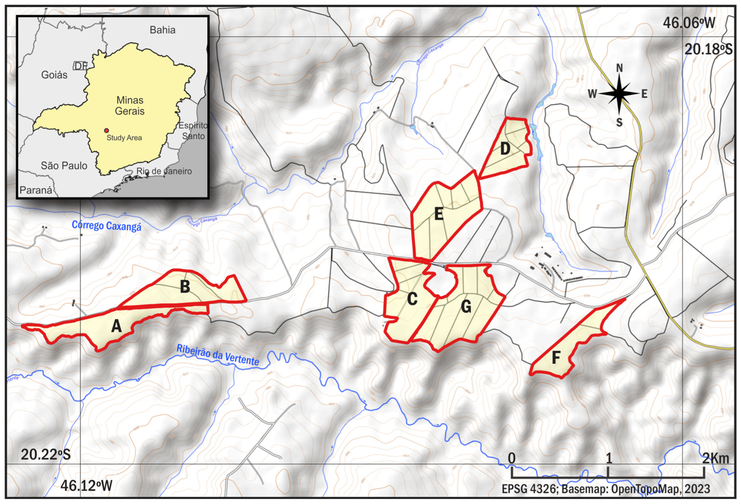
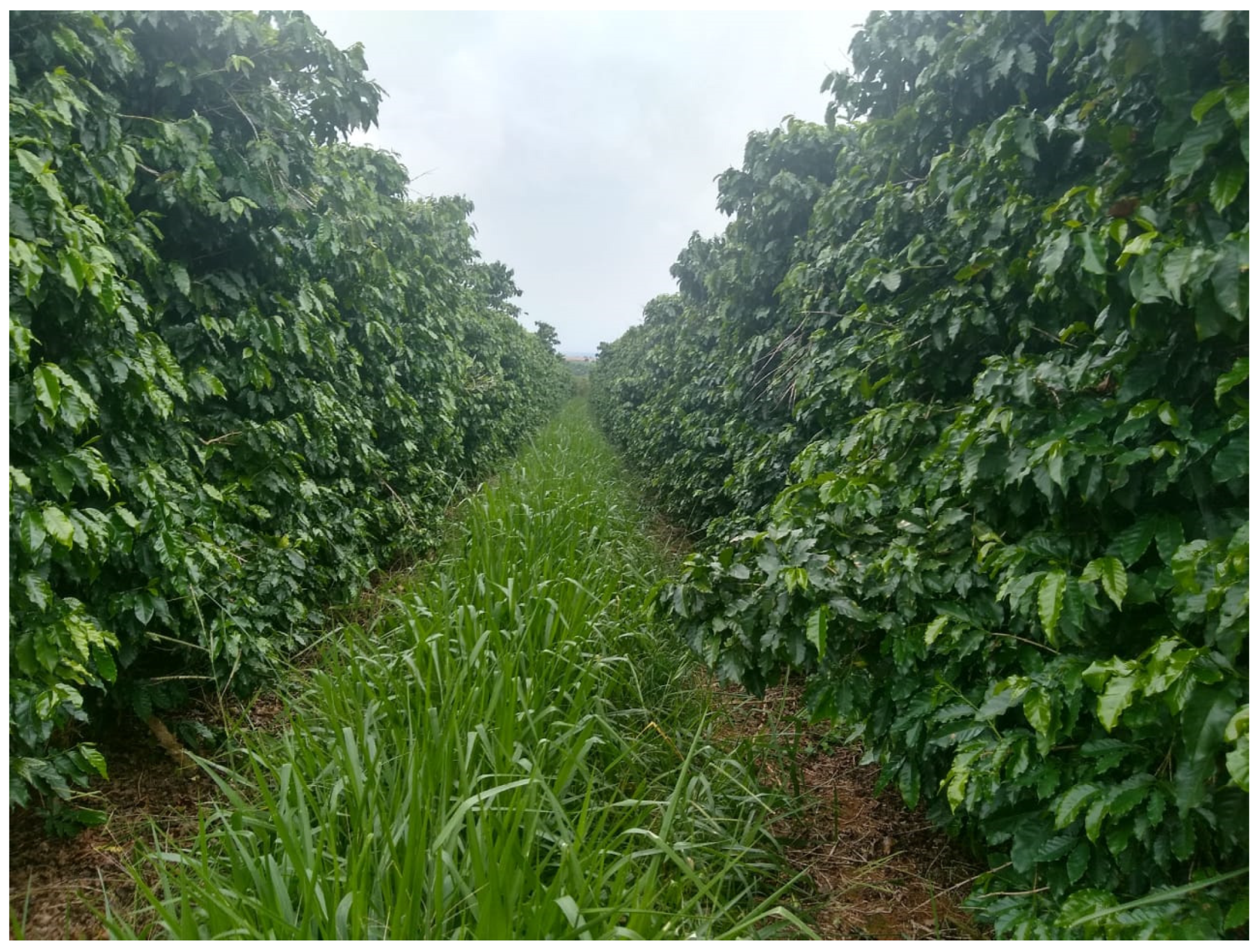
2.1. Study Area
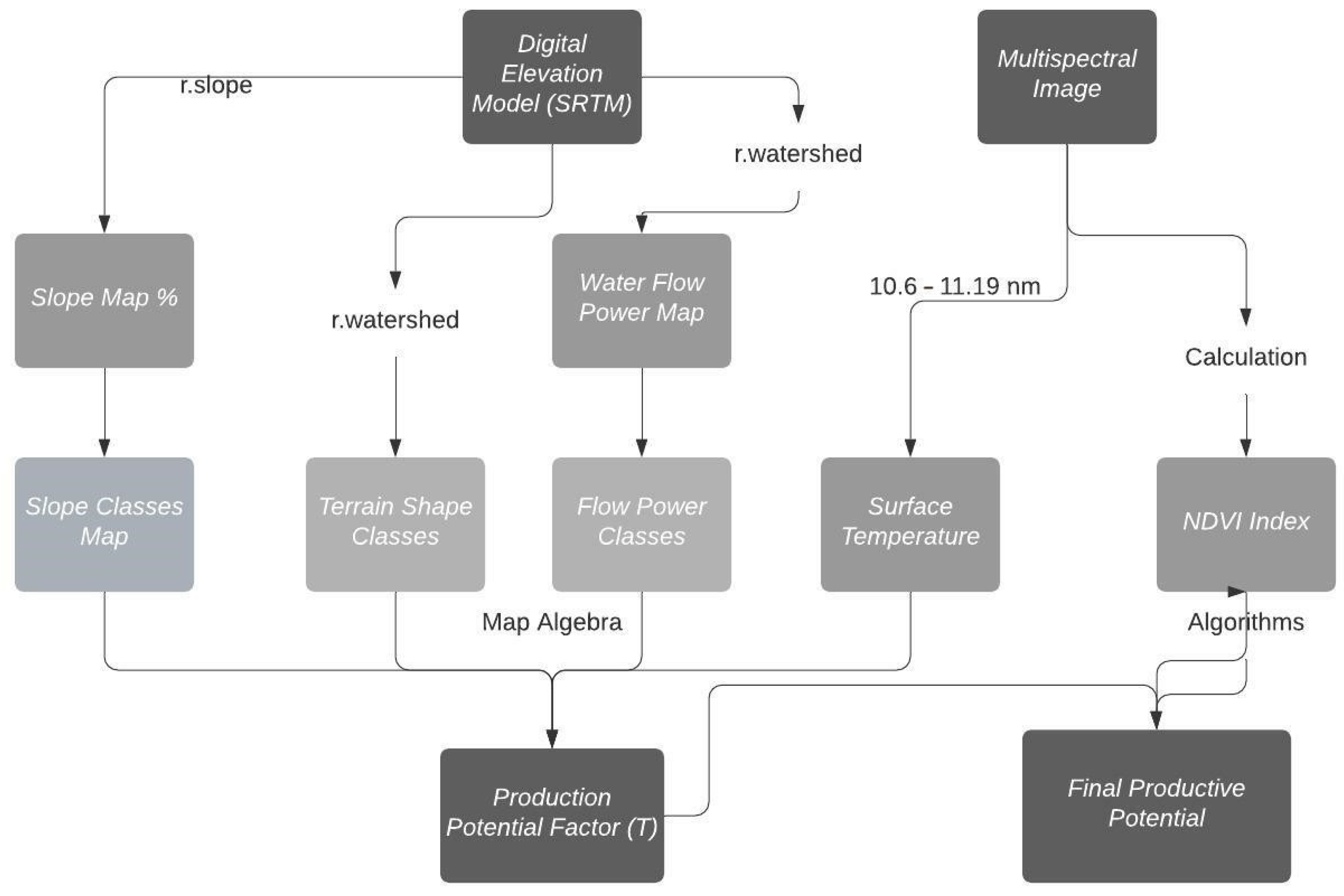
2.2. Method
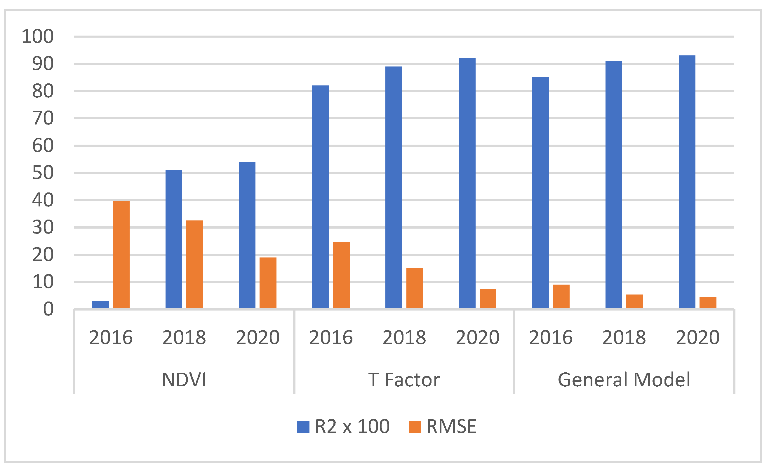
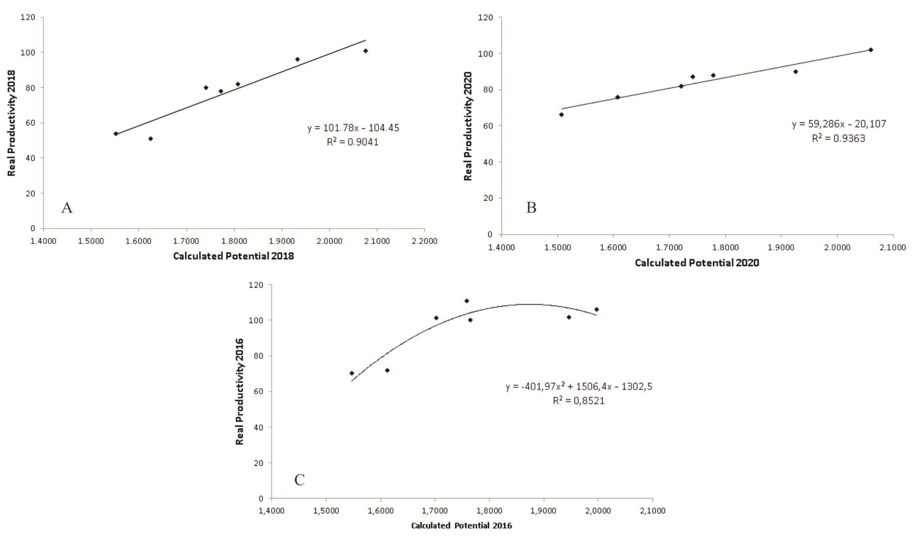
2.3. Analysis of Results
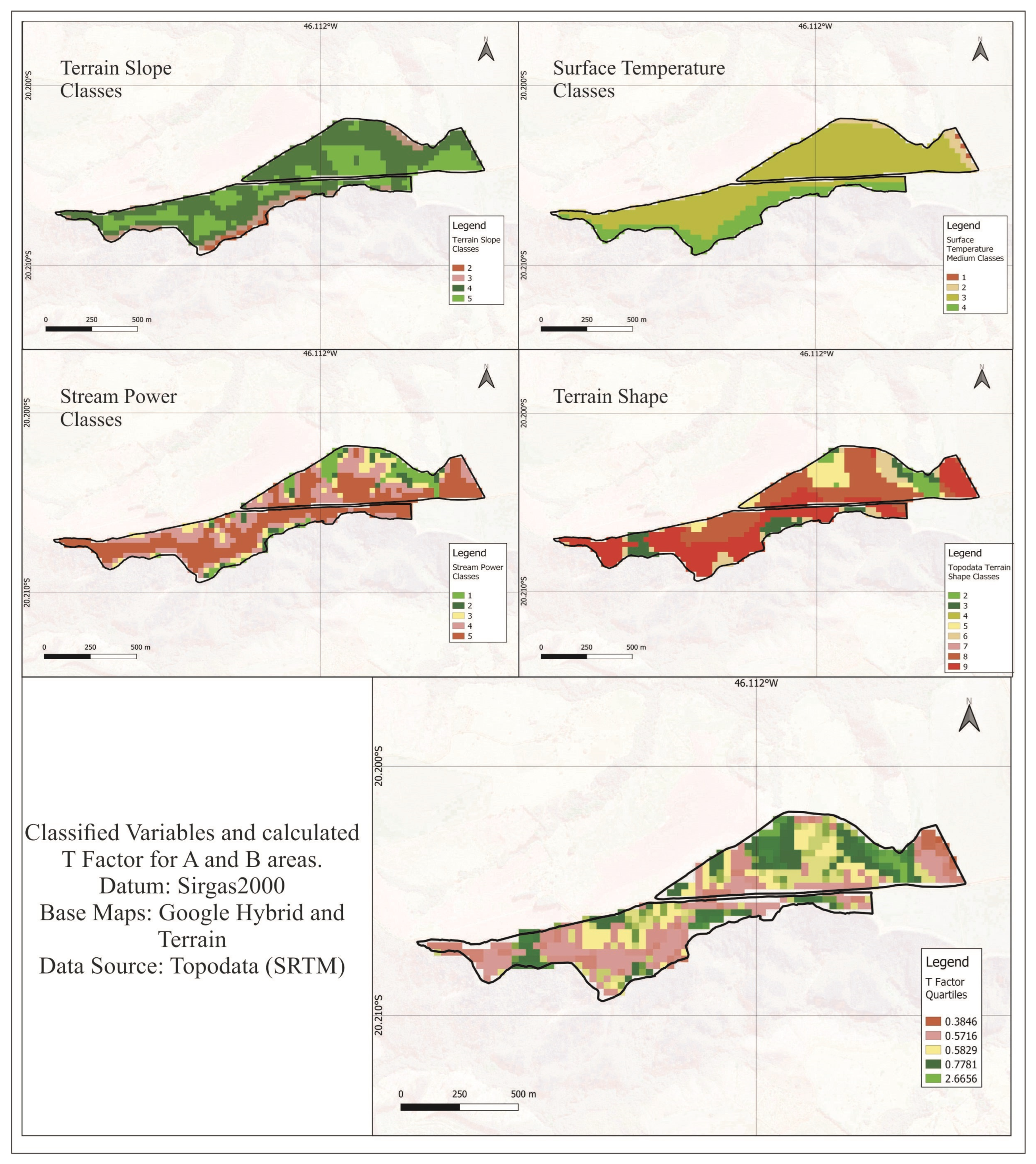
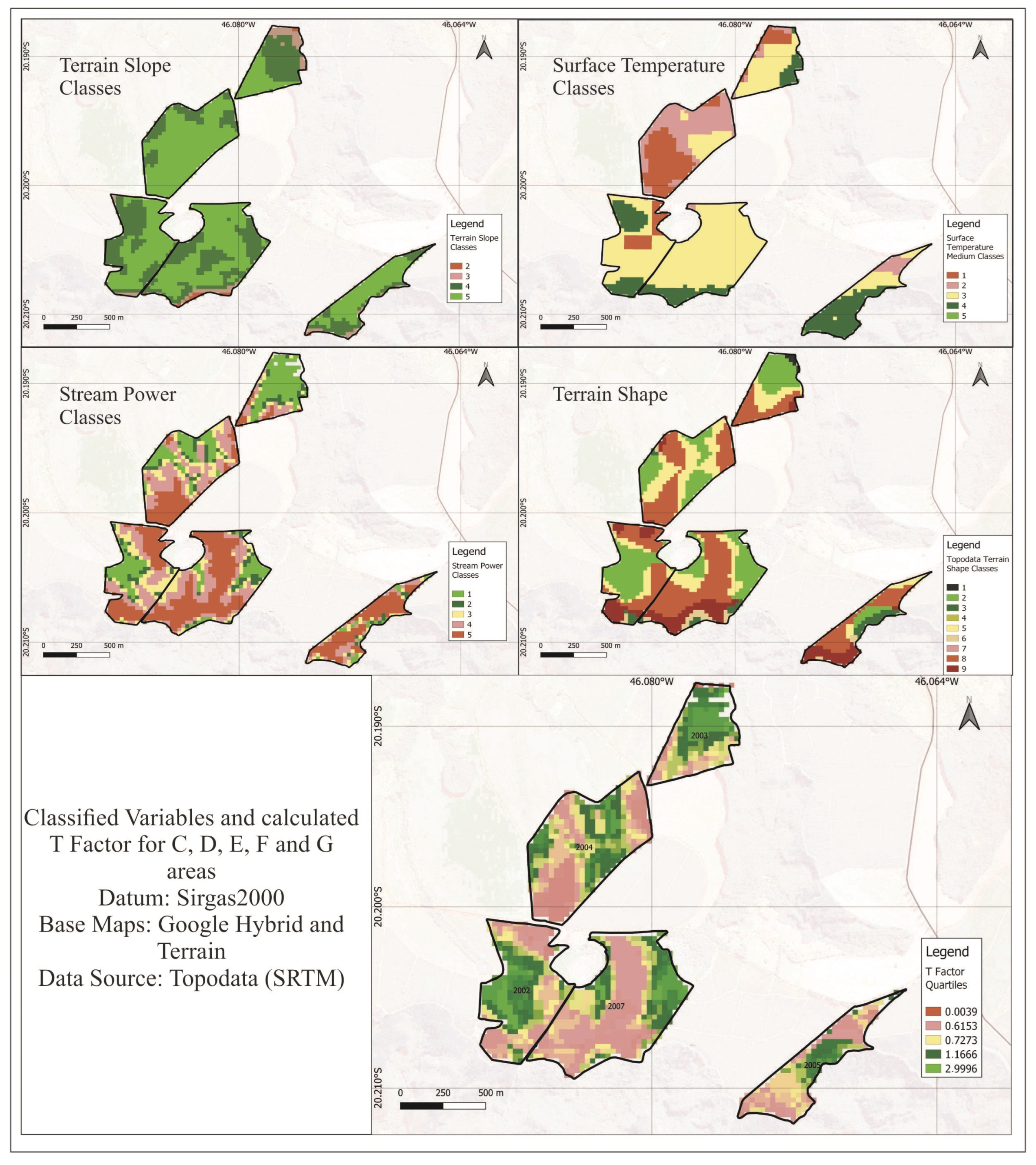
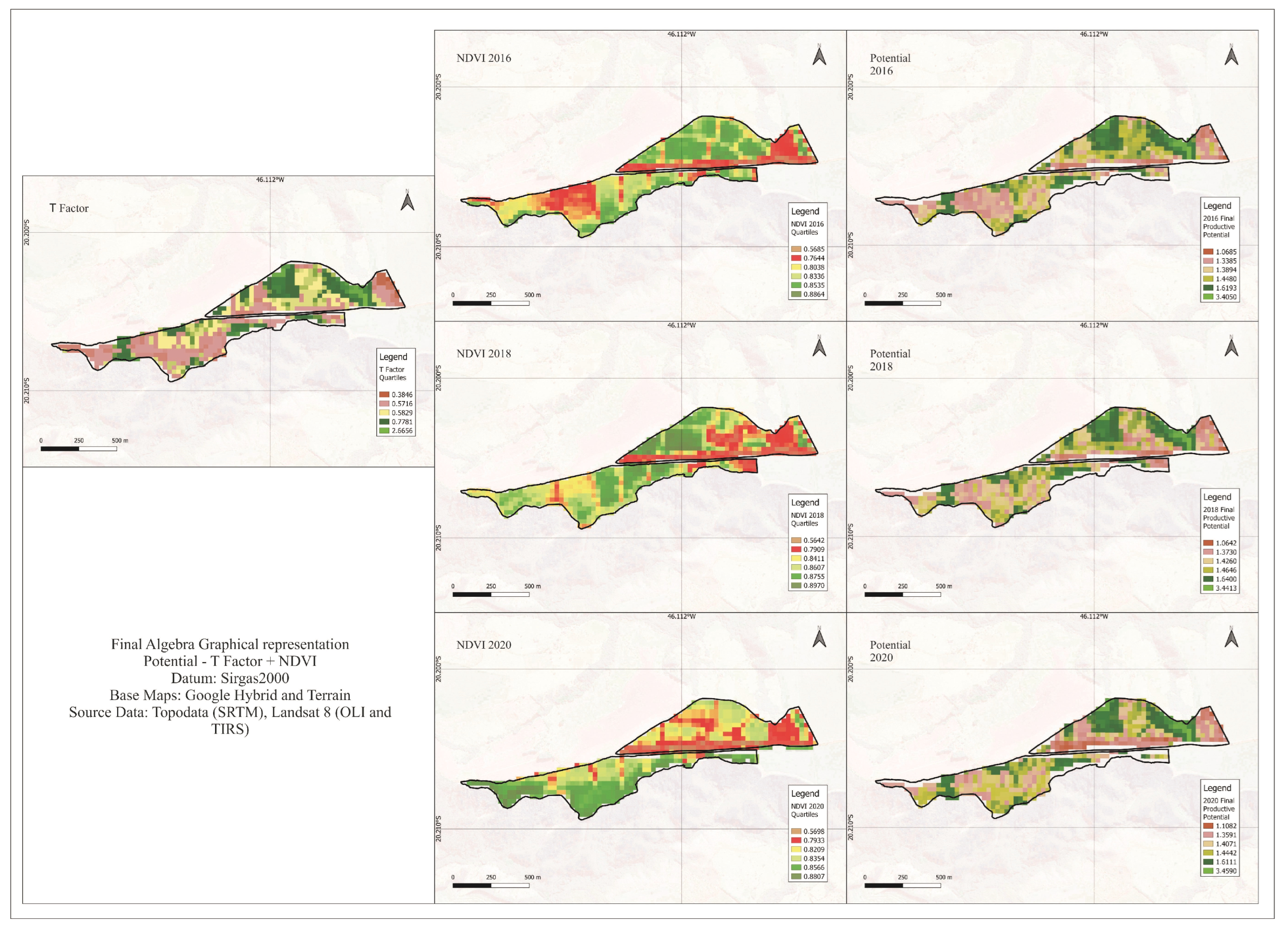
3. Results and Discussion
4. Conclusions
Supplementary Materials
Author Contributions
Funding
Data Availability Statement
Conflicts of Interest
References
- Mullan, B.; Haqq-Misra, J. Population Growth, Energy Use, and the Implications for the Search for Extraterrestrial Intelligence. Futures 2019, 106, 4–17. [Google Scholar] [CrossRef]
- Tripathi, A.D.; Mishra, R.; Maurya, K.K.; Singh, R.B.; Wilson, D.W. Estimates for World Population and Global Food Availability for Global Health. In The Role of Functional Food Security in Global Health; Elsevier: Amsterdam, The Netherlands, 2018; pp. 3–24. ISBN 9780128131480. [Google Scholar]
- Pretty, J. Agricultural Sustainability: Concepts, Principles and Evidence. Philos. Trans. R. Soc. B Biol. Sci. 2008, 363, 447–465. [Google Scholar] [CrossRef] [PubMed]
- Crosby, L.G. Developing Sustainable Leadership Strategies to Increase Corporate Revenue. Doctoral Dissertation, Walden University, Minneapolis, MN, USA, 2016. [Google Scholar]
- Zhang, N.; Wang, M.; Wang, N. Precision Agriculture—A Worldwide Overview. In Computers and Electronics in Agriculture; Elsevier: Amsterdam, The Netherlands, 2002; Volume 36, pp. 113–132. [Google Scholar]
- Gardezi, M.; Stock, R. Growing Algorithmic Governmentality: Interrogating the Social Construction of Trust in Precision Agriculture. J. Rural Stud. 2021, 84, 1–11. [Google Scholar] [CrossRef]
- Bongiovanni, R.; Lowenberg-Deboer, J. Precision Agriculture and Sustainability. Precis. Agric. 2004, 5, 359–387. [Google Scholar] [CrossRef]
- Sentelhas, P.C.; Battisti, R.; Sako, H.; Rodrigues, L.A. Clima e Produtividade Da Soja: Variabilidade Climática Como Fator Controlador Da Produtividade. Bol. Pesqui. 2018, 1, 25–41. [Google Scholar]
- Crave, A.; Gascuel-Odoux, C. The Influence of Topography on Time and Space Distribution of Soil Surface Water Content. Hydrol. Process. 1997, 11, 203–210. [Google Scholar] [CrossRef]
- Schnabel, S.; Dahlgren, R.A.; Moreno-Marcos, G. Soil and Water Dynamics; Springer: Berlin/Heidelberg, Germany, 2013; ISBN 9789400767072. [Google Scholar]
- Silva, S.; Queiroz, D.; Santo, N.; Pinto, F. Influence of Climate, Soil, Topography and Variety on the Terroir and on Coffee Quality. J. Exp. Agric. Int. 2018, 24, 1–15. [Google Scholar] [CrossRef]
- Mintesnot, A.; Dechassa, N.; Mohammed, A. Association of Arabica Coffee Quality Attributes with Selected Soil Chemical Properties. East Afr. J. Sci. 2015, 9, 73–84. [Google Scholar]
- Sanchez, M.G.B. Relação Solo-Relevo Em Áreas Sob Cultivo de Café No Sudoeste de Minas Gerais. Master’s Thesis, São Paulo State University, São Paulo, Brazil, 2009. [Google Scholar]
- Sanchez, R.B.; Marques Júnior, J.; Pereira, G.T.; Souza, Z.M. de Variabilidade Espacial de Propriedades de Latossolo e Da Produção de Café Em Diferentes Superfícies Geomórficas. Rev. Bras. Eng. Agrícola E Ambient. 2005, 9, 489–495. [Google Scholar] [CrossRef]
- Boschini, A.P.M. Produtividade e Qualidade de Grãos de Trigo Influenciados Por Nitrogênio e Lâminas de Água No Distrito Federal; UNB: Fredericton, NB, Canada, 2010; Volume 2, ISBN 0113968310. [Google Scholar]
- Evans, L.T.; Fischer, R.A. Yield Potential: Its Definition, Measurement, and Significance. Symp. ASA Meet. 1999, 1551, 1544–1551. [Google Scholar] [CrossRef]
- Rogers, M. The Definition and Measurement of Productivity; Melbourne Institute of Applied Economic and Social Research: Melbourne, Australia, 1998. [Google Scholar]
- Saito, M. Sustainable Coffee Production. In Coffee: Growing, Processing, Sustainable Production: A Guidebook for Growers, Processors, Traders, and Researchers; Wiley: Hoboken, NJ, USA, 2008; pp. 384–390. [Google Scholar] [CrossRef]
- Capa, D.; Pérez-Esteban, J.; Masaguer, A. Unsustainability of Recommended Fertilization Rates for Coffee Monoculture Due to High N2O Emissions. Agron. Sustain. Dev. 2015, 35, 1551–1559. [Google Scholar] [CrossRef]
- de Mesquita, C.M.; de Rezende, J.E.; Carvalho, J.S.; Fabri Júnior, M.A.; Moraes, N.C.; Dias, P.T.; de Carvalho, R.M.; Araújo, W.G. de MANUAL DO CAFÉ: Colheita e Preparo; Emater: Belo Horizonte, Brazil, 2016; p. 52. [Google Scholar]
- Valle Junior, R.F.; Varandas, S.G.P.; Sanches Fernandes, L.F.; Pacheco, F.A.L. Environmental Land Use Conflicts: A Threat to Soil Conservation. Land Use Policy 2014, 41, 172–185. [Google Scholar] [CrossRef]
- Lal, R.; Bouma, J.; Brevik, E.; Dawson, L.; Field, D.J.; Glaser, B.; Hatano, R.; Hartemink, A.E.; Kosaki, T.; Lascelles, B.; et al. Soils and Sustainable Development Goals of the United Nations: An International Union of Soil Sciences Perspective. Geoderma Reg. 2021, 25, e00398. [Google Scholar] [CrossRef]
- Taghizadeh-Mehrjardi, R.; Nabiollahi, K.; Rasoli, L.; Kerry, R.; Scholten, T. Land Suitability Assessment and Agricultural Production Sustainability Using Machine Learning Models. Agronomy 2020, 10, 573. [Google Scholar] [CrossRef]
- Barbosa, C.C.F.; Novo, E.M.L.M.; Martins, V.S. Introdução Ao Sensoriamento Remoto; LabISA/INPE: São José dos Campos, Brazil, 2019; ISBN 9788517000959. [Google Scholar]
- Vieira, T.G.C.; Alves, H.M.R.; Lacerda, M.P.C.; Veiga, R.D.; Epiphanio, J.C.N. Crop Parameters for the Evaluation of the Spectral Response of Coffee (Coffea Arabica) Areas within the State of Minas Gerais, Brazil. Int. Arch. Photogramm. Remote Sens. Spat. Inf. Sci. ISPRS Arch. 2004, 35, 111–118. [Google Scholar]
- da Anjinho, P.S.; Barbosa, M.A.G.A.; Costa, C.W.; Mauad, F.F. Environmental Fragility Analysis in Reservoir Drainage Basin Land Use Planning: A Brazilian Basin Case Study. Land Use Policy 2021, 100, 104946. [Google Scholar] [CrossRef]
- Manfré, L.A.; da Silva, A.M.; Urban, R.C.; Rodgers, J. Environmental Fragility Evaluation and Guidelines for Environmental Zoning: A Study Case on Ibiuna (the Southeastern Brazilian Region). Environ. Earth Sci. 2013, 69, 947–957. [Google Scholar] [CrossRef]
- Massa, E.M.; Ross, J.L.S. Aplicação De Um Modelo De Fragilidade Ambiental Relevo-Solo Na Serra Da Cantareira, Bacia Do Córrego Do Bispo, São Paulo-Sp. Geogr. Dep. Univ. Sao Paulo 2012, 24, 57–79. [Google Scholar] [CrossRef]
- Oliveira-Andreoli, E.Z.; de Moraes, M.C.P.; da Faustino, A.S.; Vasconcelos, A.F.; Costa, C.W.; Moschini, L.E.; Melanda, E.A.; Justino, E.A.; Di Lollo, J.A.; Lorandi, R. Multi-Temporal Analysis of Land Use Land Cover Interference in Environmental Fragility in a Mesozoic Basin, Southeastern Brazil. Groundw. Sustain. Dev. 2021, 12, 100536. [Google Scholar] [CrossRef]
- Schaefer, C.E.G.R. Bases Físicas Da Paisagem Brasileira: Estrutura Geológica, Relevo e Solos. Tópicos Em Ciência Do Solo 2013, 8, 221–278. [Google Scholar]
- Torrado, P.V.; Lepsch, I.F.; de Castro, S.S. Conceitos e Aplicações Das Relações Pedologia-Morfologia Em Regiões Tropicais Úmidas; Sociedade Brasileira de Ciência do Solo: Viçosa, MG, Brazil, 2005. [Google Scholar]
- de Morisson Valeriano, M.; de Fátima Rossetti, D. Topodata: Brazilian Full Coverage Refinement of SRTM Data. Appl. Geogr. 2012, 32, 300–309. [Google Scholar] [CrossRef]
- da Silva, F.M.; de Souza, Z.M.; de Figueiredo, C.A.P.; Marques Júnior, J.; Machado, R.V. Variabilidade Espacial de Atributos Químicos e de Produtividade Na Cultura Do Café. Ciência Rural 2007, 37, 401–407. [Google Scholar] [CrossRef]
- de Souza, Z.M.; Marques Júnior, J.; Pereira, G.T.; Moreira, L.F. Variabilidade Espacial Do PH, Ca, Mg e V% Do Solo Em Diferentes Formas Do Relevo Sob Cultivo de Cana-de-Açúcar. Ciência Rural 2004, 34, 1763–1771. [Google Scholar] [CrossRef]
- Bernardes, T.; Moreira, M.A.; Adami, M.; Rudorff, B.F.T. Physic-Environmental Diagnosis of Coffee Crop in the State of Minas Gerais, Brazil. Coffee Sci. 2012, 7, 139–151. [Google Scholar]
- Martins, V.E.; Da Silva, D.M.; Gass, S.L.B. Correção Atmosférica De Imagens De Satélite Para Fins De Mapeamento Temporal De Uso E Cobertura Do Solo. XXV Semin. Iniciação Científica 2017. [Google Scholar]
- Seelan, S.K.; Laguette, S.; Casady, G.M.; Seielstad, G.A. Remote Sensing Applications for Precision Agriculture: A Learning Community Approach. Remote Sens. Environ. 2003, 88, 157–169. [Google Scholar] [CrossRef]
- Damasceno, V.G.; Torres Fernandes, A.F.; dos Neto, C.F.S.; da Rodrigo, S.G.; Cândido, M.J.D. Estimativa do potencial produtivo de forrageiras exóticas índice de vegetação normalized difference vegetation index (ndvi) for estimate the productive potential of exotic forages. Educ. Ciência Tecnol. e Amor. 2020, 1–17. [Google Scholar] [CrossRef]
- Santos, G.O.; Rosalen, D.L.; De Faria, R.T. Use of Active Optical Sensor in the Characteristics Analysis of the Fertigated Brachiaria with Treated Sewage. Eng. Agric. 2017, 37, 1213–1221. [Google Scholar] [CrossRef]
- Schneitz, K.; Sablowski, R.; Lemieux, B.; Dunwell, J.; Sweetlove, L.; Fernie, A.; Metraux, J.-P.; Palme, K.; McAinsh, M.R.; Weisshaar, B.; et al. Plant Biology. Curr. Opin. Plant Biol. 2002, 5, 265–274. [Google Scholar]
- De Souza, Z.M.; Marques, J.; Pereira, G.T.; Barbieri, D.M. Small Relief Shape Variations Influence Spatial Variability of Soil Chemical Attributes. Sci. Agric. 2006, 63, 161–168. [Google Scholar] [CrossRef]
- Rossi, M.; Queiroz Neto, J.P. Relação Solo/Paisagem Em Regiões Tropicais Úmidas: O Exemplo Da Serra Do Mar Em São Paulo, Brasil. Geogr. Dep. Univ. Sao Paulo 2001, 14, 11–23. [Google Scholar] [CrossRef]
- Carvalho, H.F. Genomic Prediction in Arabica Coffee Considering Bienniality and Threshold Models. Doctoral Dissertation, Instituto Agronômico de Campinas, Campinas, Brazil, 2019. [Google Scholar]
- Vieira Júnior, I.C.; Da Silva, C.P.; Nuvunga, J.J.; Botelho, C.E.; Gonçalves, F.M.A.; Balestre, M. Mixture Mixed Models: Biennial Growth as a Latent Variable in Coffee Bean Progenies. Crop Sci. 2019, 59, 1424–1441. [Google Scholar] [CrossRef]
- Nogueira, S.M.C.; Moreira, M.A.; Volpato, M.M.L. Relationship between Coffee Crop Productivity and Vegetation Indexes Derived from OLI/Landsat-8 Sensor Data with and without Topographic Correction. Int. Braz. Assoc. Agric. Eng. 2018, 38, 387–394. [Google Scholar] [CrossRef]
- Hunt, D.A.; Tabor, K.; Hewson, J.H.; Wood, M.A.; Reymondin, L.; Koenig, K.; Schmitt-Harsh, M.; Follett, F. Review of Remote Sensing Methods to Map Coffee Production Systems. Remote Sens. 2020, 12, 2041. [Google Scholar] [CrossRef]
- Fanelli Carvalho, H.; Galli, G.; Ventorim Ferrão, L.F.; Vieira Almeida Nonato, J.; Padilha, L.; Perez Maluf, M.; Ribeiro de Resende, M.F.; Guerreiro Filho, O.; Fritsche-Neto, R. The Effect of Bienniality on Genomic Prediction of Yield in Arabica Coffee. Euphytica 2020, 216, 1–16. [Google Scholar] [CrossRef]


| Data | Type | Source | References |
|---|---|---|---|
| Digital Elevation Model | Raster Image | Topodata–Inpe | Valeriano [32] |
| Multispectral Image (NDVI) | Raster Image | Copernicus–ESA | |
| Spectral Image (Thermal) | Raster Image | USDA–NASA | |
| Slope Shape | Raster Image | Topodata–Inpe | Valeriano [32] |
| Hierarchical Categories | Declivity (%) | Flow Power (W/m) | Terrain Shape (Topodata Classes) | Temperature (Celsius) |
|---|---|---|---|---|
| Very bad | >25 (1) | 0–2 (1) | 8 and 9 (1) | >20.13 (1) |
| Bad | 16–25 (2) | 2–4 (2) | 6 and 7 (2) | 19.90–20.13 (2) |
| Medium | 12–16 (3) | 4–6 (3) | 4 and 5 (3) | 19.67–19.90 (3) |
| Good | 0–2 and 6–12 (4) | 6–8 (2) | 1 and 3 (2) | 19.44–19.67 (4) |
| Very Good | 3–6 (5) | >8 (1) | 2 (1) | 19.00–19.44 (5) |
| Plot | Productivity (Benefited Bags.hectare−1) | Standard Deviation (Benefited Bags.hectare−1) | |||
|---|---|---|---|---|---|
| 2016 | 2018 | 2020 | Medium | ||
| D | 106 | 101 | 102 | 61.80 | 2.65 |
| C | 102 | 96 | 90 | 57.50 | 5.76 |
| G | 111 | 82 | 88 | 56.17 | 15.23 |
| F | 100 | 80 | 87 | 53.40 | 10.15 |
| E | 101 | 78 | 82 | 52.26 | 12.47 |
| B | 72 | 51 | 76 | 39.73 | 13.36 |
| A | 70 | 54 | 66 | 38.07 | 8.46 |
| Medium | 95 | 77 | 84 | 85.33 | |
| Standard Deviation | 16.49 | 19.04 | 11.37 | ||
| Variable | R2 | Equation |
|---|---|---|
| Terrain Shape | 0.7723 | y = −7.6959x + 98.66 |
| Water Flow Power | 0.4144 | y = 8.3527ln(x) + 35.082 |
| NDVI | 0.3908 | y = 303.46x − 206.23 |
| Slope | 0.1073 | y = −0.7107x2 + 7.1845x + 35.273 |
| Data/Plot | A | B | C | D | E | F | G |
|---|---|---|---|---|---|---|---|
| Terrain Shape | 7.77 | 6.91 | 5.35 | 4.81 | 5.46 | 6.64 | 6.16 |
| Flow Power | 4.29 | 3.7 | 3.41 | 2.06 | 3.36 | 4.08 | 3.95 |
| Declivity | 4 | 4 | 5 | 4 | 5 | 5 | 5 |
| Temperature | 4.45 | 4.49 | 3.28 | 4.68 | 4.39 | 4.23 | 4.66 |
| T Factor | 0.70 | 0.80 | 0.93 | 0.90 | 1.07 | 1.19 | 0.95 |
| NDVI medium 2018 | 0.8514 | 0.8242 | 0.8621 | 0.8788 | 0.8328 | 0.8384 | 0.8522 |
| NDVI medium 2020 | 0.8461 | 0.8120 | 0.8742 | 0.7991 | 0.7640 | 0.8613 | 0.8024 |
| NDVI medium 2016 | 0.8066 | 0.8076 | 0.8539 | 0.8621 | 0.7822 | 0.8388 | 0.8226 |
Disclaimer/Publisher’s Note: The statements, opinions and data contained in all publications are solely those of the individual author(s) and contributor(s) and not of MDPI and/or the editor(s). MDPI and/or the editor(s) disclaim responsibility for any injury to people or property resulting from any ideas, methods, instructions or products referred to in the content. |
© 2023 by the authors. Licensee MDPI, Basel, Switzerland. This article is an open access article distributed under the terms and conditions of the Creative Commons Attribution (CC BY) license (https://creativecommons.org/licenses/by/4.0/).
Share and Cite
Cunha, J.E.F.; Martins, G.D.; Fraga Júnior, E.F.; Camboim, S.P.; Bravo, J.V.M. A Multicriteria Model for Estimating Coffea arabica L. Productive Potential Based on the Observation of Landscape Elements. Agriculture 2023, 13, 2083. https://doi.org/10.3390/agriculture13112083
Cunha JEF, Martins GD, Fraga Júnior EF, Camboim SP, Bravo JVM. A Multicriteria Model for Estimating Coffea arabica L. Productive Potential Based on the Observation of Landscape Elements. Agriculture. 2023; 13(11):2083. https://doi.org/10.3390/agriculture13112083
Chicago/Turabian StyleCunha, Jorge Eduardo F., George Deroco Martins, Eusímio Felisbino Fraga Júnior, Silvana P. Camboim, and João Vitor M. Bravo. 2023. "A Multicriteria Model for Estimating Coffea arabica L. Productive Potential Based on the Observation of Landscape Elements" Agriculture 13, no. 11: 2083. https://doi.org/10.3390/agriculture13112083