Time, Spatial and Component Characteristics of Agricultural Carbon Emissions of China

Abstract

In this study, the time trend, regional distribution and component characteristics of the agricultural carbon emissions (ACEs) of China are analyzed. The estimation methods of each component of the ACE are introduced. According to the annually provincial panel data set with the 31 provinces from 1996 to 2019, the time trend, regional distribution and component characteristics are empirically discussed. Meanwhile, since it is also worthwhile to explore the effect of the ACE on economic growth, econometric models such as the pooled ordinary least squares (OLS) and fixed effect (FE) models are employed to examine the inverted “U”-shape effect of ACE on both of the agricultural GDP and GDP under the control of other variables. The results show that (1) the carbon emission started to fall after 2015; (2) the majority source of the agricultural carbon emission is caused by chemical fertilizer, which is approximately half of the total; (3) the current provincial ACE levels (0.287 $\times {10}^{10}$ kg in 2019) are significantly smaller than the estimated optimal level for agricultural GDP as well as GDP (respectively, $1.003\times {10}^{10}$ kg and $1.256\times {10}^{10}$ kg). In light of this, environmental protection and agricultural development are currently conflicted. Therefore, we suggest that the government should accept a trade-off between economic growth and the quality of the environment.

1. Introduction

According to the greenhouse gas emissions in 2019 provided by the World Bank, China ranks first in the world in greenhouse gas emissions, and the volume is approximately 1/3 of the world total. Because of this, some people believe that one of the main causes of global warming is the massive emission of greenhouse gases in China. At the United Nations General Assembly, China announced to the world that it would strive to achieve carbon peak by 2030 and carbon neutrality by 2020. It is generally believed that the industrial sector is the main source of carbon emissions, and agricultural carbon emission is the issue that is easy to be commonly ignored. According to the statistics of the Food and Agriculture Organization of the United Nations (FAO), the carbon emissions from agricultural production and land use have accounted for 1/4 of the total carbon emissions from human activities, and agricultural greenhouse gas emissions are an important part of the total carbon emissions [1]. Agriculture is an important part of China’s national economy. Because of the largest population, China’s agricultural carbon emission is higher than the world average. The total agricultural carbon emissions account for 29% of the total agricultural carbon emissions in Asia and about 13% of the world total. Planting plays a particularly important role in agriculture and is a major component of agriculture industry. In a narrow sense, agriculture is the planting industry, including the production of food crops, cash crops, feed crops, green manure and other crops. Under the background of the current low-carbon economy, China’s fast-growing planting industry has also exposed a series of problems, such as excessive use and low efficiency of agricultural production materials such as chemical fertilizers, pesticides, agricultural film, high carbon emissions, soil and water resources pollution, and deteriorating ecological environment. Therefore, promoting the low-carbon development of the planting industry is an inevitable problem in current theoretical research and actual production. Recently, three major issues should be theoretically and empirically clarified. First, what are the geographical distribution and time trend of the agricultural carbon emission of China? We should focus our research on areas with relatively high carbon emissions and a significant trend of growth. Second, what are the determinants of the agricultural carbon emissions? Some areas may be due to the expansion of agricultural scale, but some others may be due to low agricultural efficiency. Third, what is the relation between agricultural carbon emission and agricultural GDP growth? Although carbon emission reduction is the purpose of this research, we should also take into account the actual needs of agricultural development.

2. Literature Review

According to the report issued by the World Meteorological Organization, the global average annual temperature increased by 0.7 centigrade in the 100 years from the end of the 19th century to the end of the 20th century. This is one of the main reasons that many scholars pay attention to carbon emissions in recent years. According to the second assessment report of the Intergovernmental Panel on Climate Change (IPCC) of the United Nations, the largest global greenhouse gas emissions come from energy use, accounting for 24%. Secondly, deforestation was converted into land, accounting for 18%. Agriculture, industry and transportation all ranked third, accounting for 14% each [2]. Academia began to study carbon emissions as early as the 1980s, but it was not until the beginning of the 21st century that the concept of agricultural carbon emissions was really put forward and studied in depth. China is a large agricultural country, so agriculture is the most important basic industry in China. The total carbon emissions of China’s farmland ecosystem account for 16–17% of China’s total greenhouse gas emissions [3].

The definition of agricultural carbon emissions is a problem that needs to be clarified first. It should be known that agriculture, especially the planting industry, has two functions: carbon source and carbon sink [4]. Simply speaking, on one hand, the respiration of crops, the decay of organic matter, and human agricultural activities such as the use of agricultural machinery will cause carbon emissions. On the other hand, carbon will also be retained during crop growth and organic matter decomposition and burial. In other words, from this point of view, there is an obvious difference between agricultural carbon emissions and those of other industries such as manufacturing and transportation industries. In light of this, the agricultural carbon emissions refer to the carbon emissions from agricultural activities such as the use of agricultural machinery, the manufacture and use of chemical fertilizers, and electric irrigation rather than the net carbon emissions from crops [5]. Therefore, the method for estimating agricultural carbon emissions is simply to estimate the total agricultural carbon emissions based on the carbon emissions of various agricultural activities.

The classification and measurement method of agricultural carbon emissions has also been established in the past two decades. In the early research, there was no consensus on the classification definition of agricultural carbon emissions. West and Marland [6] divide agricultural carbon emissions into four categories: fertilizer, pesticide, irrigation and seed cultivation, and then measures their carbon emissions in each category. Johnson et al. [7] stated that the sources of agricultural carbon emissions should be also four categories: agricultural waste abnormal treatment, livestock breeding, agricultural energy utilization and plant growth. In contrast, Mosier et al. [8] divides agricultural carbon emissions into three parts: land use, plant growth and animal breeding. Compared among these three, we can find that their definitions are quite close with slight differences. The Intergovernment Panel on Climate Change (IPCC) gives the estimation method of agricultural carbon emissions and the corresponding estimation coefficient [2,9]. The carbon emission sources of the planting industry mainly come from six aspects: the production and use of the chemical fertilizer, the production and use of the pesticide, the production and use of the agricultural film, the use of the diesel for agricultural machinery, carbon emission from irrigation and land ploughing. Some argued that two categories, the use of the diesel for agricultural machinery and land ploughing, should be taken into account in one category as the purpose of using agricultural machinery is for agricultural activities. So, for this academic issue, we also support the view that there are five categories of the main sources of the agricultural carbon emissions [10,11]. Meanwhile, some studies focus on some other sources of the agricultural carbon emission such as the biogas generated in the water area, methane produced by livestock, decay caused by rain and agricultural waste [12]. However, results show that they are too tiny compared with the above five main sources of the agricultural carbon emissions.

Holka et al. [13] demonstrated that the production and use of the chemical fertilizer is the main source of the agricultural carbon emission, and the development of the organic farming effectively reduces the use of the chemical fertilizer and thus decreases carbon emissions. Wen et al. [14] found that the provincial levels of the structure (proportions) of the six sources of the agricultural carbon emissions of the 31 provinces converged during the recent years. Some [15,16] also found this kind of convergence effect and called this the “agglomeration effect”. Liu and Yang [17] explored the spatial spillover effect by the spatial econometric models and illustrated that the Moran’s I index was reduced from 2009 to 2019, which implies that the convergence effect was practically reduced in recent years. In light of this, it is necessary to carefully think about the temporal–spatial characteristics of the agricultural carbon emissions.

Some studies focused on the relationship between agricultural carbon emissions and economic growth. Zhao et al. [18] conducted research on the effect of China’s agricultural carbon emission on the effectiveness of the agricultural industry and found that government expenditure and residents’ income have positive effects on the elasticity of agricultural carbon emission to agricultural GDP. Li and Zhou [19] explored the role of technology in the effect between the agricultural GDP and agricultural carbon emission, and they found that technology has a positive effect on the reduction of the agricultural carbon emission. Li et al. [20] found that the rise in agricultural ecological efficiency will cause sustainable and high-quality agricultural development. Given by the coupling coordination model, Xia et al. [21] found that there is a significant positive relation between agricultural carbon emission and agricultural development, and this effect is relatively larger in northern China. Han et al. [22] also apply the coupling model and found evidence that the relationship between agricultural carbon emission and agricultural development is relatively high in the middle and low in western China. Some also theoretically introduced and empirically confirmed the inverted “U”-shape relation between agricultural carbon emission and GDP per capita described by the environmental Kuznets theory [10,23]. Zhang et al. [24] focused on this issue and found evidence that China’s agricultural carbon emission indeed showed a inverted “U” shape with economic development at the provincial level panel data.

There are also lots of related works. Yang et al. [25] found significant positive spatial spillover effect in the carbon emissions, and therefore, they believed that local environmental governance is more important. He et al. [26] also concentrated on the spatial spillover effect and found evidence that local governments with a low level of economic development tend to follow the carbon emission reduction policies provided by the highly developed surrounding regions. Guo et al. [27] found that financial support will directly affect the agricultural carbon emissions and will also indirectly affect the agricultural carbon emission through the use of chemical fertilizer. Tian et al. [28] explored the driving factors of the agricultural carbon emission by the LMDI model and stated that the changed agricultural efficiency, labor and structure factors cause a significant reduction in the agricultural carbon emissions. Zhang et al. [29] measured the agricultural carbon emission efficiency based on the SBM–DEA model and found that China’s technological efficiency is in an “efficient” state for the agricultural industry. Zhao et al. [30] found a “water–land–energy–carbon nexus” in the issue of agricultural carbon emission.

There are still some shortcomings in the existing research. First, among the three important perspectives (time trend, regional distribution and carbon sources) of the agricultural carbon emissions, most of the related studies only consider one or two aspects. For example, Hu et al. [31] only considered the spatial and temporal characteristics of one province—Jiangsu—of China. Xiong et al. [32,33] explored the spatial and temporal characteristics of the agricultural carbon emission only for the Hotan prefecture of China. Second, because the environmental Kuznets curve is a famous theory, most related studies only focus on the causal effect of the agricultural GDP per capita, GDP per capita or individual’s disposable income on agricultural carbon emission. Few works are concentrated on the effect of agricultural carbon emission on the agricultural GDP as well as the GDP.

Therefore, this article is organized as follows. In Section 3, data and methods are described. The methods of estimating the agricultural carbon emission and the method of estimating the effect of agricultural carbon emissions on the agricultural GDP and the GDP are introduced. Vivid figures are given in Section 4, and the characteristics of the agricultural carbon emission of China will be analyzed. Section 5 is the conclusion section where conclusions, policy suggestions and limitations are summarized.

3. Data and Method

In this section, there are three subsections. The first subsection describes the necessary information of the data set. Given by the variables, the second subsection introduces the related parameters and the estimation method of the agricultural carbon emissions (ACE). In the third subsection, empirical equations as well as the regression models are discussed for the purpose of estimating the effect of ACE on economic growth.

3.1. Data

As the research object is China’s agricultural carbon emission issue, we select nine variables, and all of these variables are available in the China Statistical Yearbook provided by China’s national statistical office (http://data.stats.gov.cn/index.htm (accessed on 1 November 2022)). Since some of the key data are not available for some provinces, and also because of the influence of the COVID-19 pandemic, data after 2020 are not considered. Under the judgement between the accuracy of results and complexity of data analysis, the provincial data are finally employed. Thus, the original data set is an annually provincial panel data with 31 provinces (expect Taiwan, Macao and Hong Kong) for the period from 1995 to 2019. More details such as the variable names, full names and scales are summarized in

Table 1. Data description.

Variable	Full Name	Scale
$AM$	Total Agricultural Machinery Power	10,000 kW
$SA$	Total Sown Area	1000 hectares; ${10}^7$ m${}^2$
$PF$	Agricultural Plastic Film	ton; 1000 kg
$PE$	Pesticide	10,000 tons; ${10}^7$ kg
$IR$	Irrigated Area of Cultivated Land	1000 hectares; ${10}^7$ m${}^2$
$FE$	Consumption of Chemical Fertilizers	10,000 tons; ${10}^7$ kg
$AGDP$	Total Output of the Primary Industry	100 million yuan
$GDP$	Gross Domestic Product	100 million yuan
$POP$	Total Population (year-end)	10,000 persons

Notes: (1) kW = Kilowatt; (2) AGDP and GDP are measured at the current price, CNY; (3) Given by the definition provided by the National Statistical Office (GB/T 4754–2017), Agricultural GDP is the Total Output of the Primary Industry, which is the Gross Output Values of Agriculture, Forestry, Animal Husbandry and Fishery excluding the Gross Output Values of the Supporting activities of Agriculture, Forestry, Animal Husbandry and Fishery; (4) Population data are available from 2000.

.

Table 2. Data description.

Variable	Obs	Mean	Std. Dev.	Min	Max
$AM$	772	2466.445	2527.492	58.500	13,353.020
$SA$	773	5117.986	3656.448	88.550	14,902.720
$PF$	773	61,255.710	60,101.608	24.000	343,524.000
$PE$	773	4.863	4.185	0.040	19.880
$IR$	773	1892.835	1487.284	109.240	6177.590
$FE$	774	161.301	133.581	1.500	716.090
$AGDP$	775	1127.477	1116.778	23.500	5477.100
$GDP$	775	11,893.243	15,395.906	56.100	107,986.900
$POP$	620	4298.669	2762.571	258.000	12,489.000

Notes: three decimal places.

shows the statistical description of the original data. Clearly, according to the number of observations of the variables, $AGDP$ and $GDP$ have no missing values (31 provinces × 25 years = 775 obs), and population has no missing data after the year 2000 (31 provinces × 20 years = 620 obs). For all of the six variables $AM$, $SA$, $PF$, $PE$, $IR$ and $FE$, effective values are quite close to 775, which implies that for each of these six variables, only one or two values are missing. In addition, these missing values are only for the province Chongqing in 1995 or 1996. In light of this, the original data set is a strongly balanced panel especially for the period from 2000 to 2019.

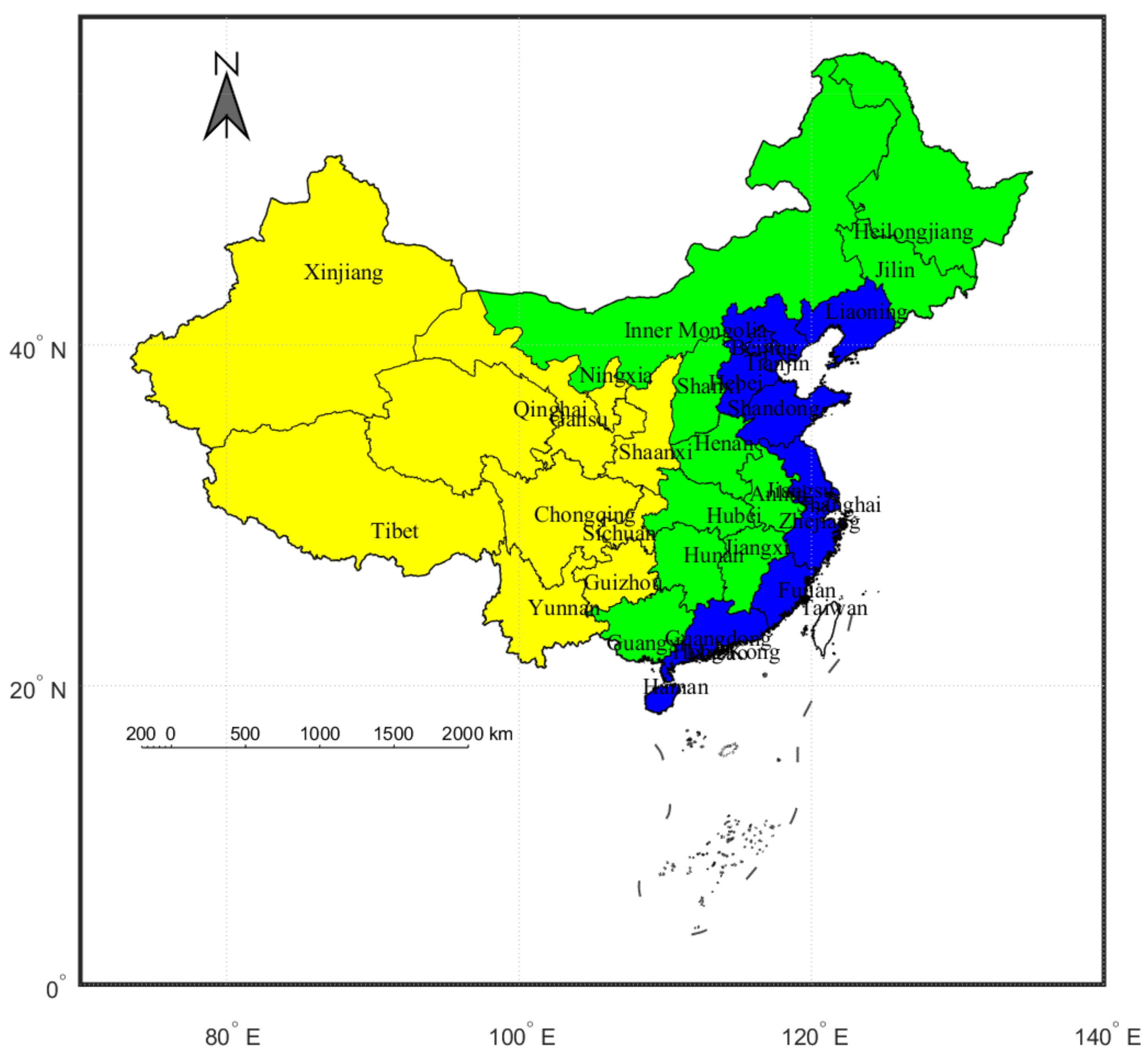
Remember that the geographical distribution is also one of our main concertations. However, we can imagine that showing the time tendencies of 31 provinces by figures would be quite disordered. Related studies would like to divide China into several regions according to the provincial geographical characteristics. China has a particularly clear geographical difference: the southeast is the plain area, the middle is the mountain area and the northwest is the high land area. Different regions have their own climatic characteristics and their own structure of agricultural products. According to The Fourth Session of the Sixth National People’s Congress, the eastern, middle and western regions, respectively, include 11, 11, and 10 provinces, as shown by Figure 1. Remember that the land areas of these three regions are not the same; for eastern, middle and western regions, their land sizes are generally $2:6:11$. Figure 1 is drawn by software Matlab with the map files (*.shp, etc.) provided by the Ministry of Natural Resources of China (DR No.: GS(2019)1822).

3.2. Estimation Method of the Agricultural Carbon Emissions (ACE)

According to the sources of the agricultural carbon emissions, total agricultural carbon emissions ($ACE$) can be generally decomposed into 5 classifications [3,26]: (1) carbon emissions of the agricultural machinery, $AC{E}_{AM}$; (2) carbon emissions of the production and use of agricultural plastic film, $AC{E}_{PF}$; (3) carbon emissions of the production and use of pesticide, $AC{E}_{PE}$; (4) carbon emissions from irrigation, $AC{E}_{IR}$; and (5) carbon emissions of the production and use of fertilizers, $AC{E}_{FE}$. Their simple mathematical relation is shown by Equation (1).

$$ACE=AC{E}_{AM}+AC{E}_{PF}+AC{E}_{PE}+AC{E}_{IR}+AC{E}_{FE}$$

(1)

Except for classification (1), for items (2) to (5), each of their carbon emissions ($AC{E}_i$) can be estimated by the amount ($Q_i$) multiplied by the carbon emission coefficient (${\alpha }_i$), which is given as $AC{E}_i={\alpha }_i\times Q_i$. For classification (1), $AC{E}_{AM}={\alpha }_{AM1}\times AM+{\alpha }_{AM2}\times SA$ where AM = total agricultural machinery power, SA = total sown area, and ${\alpha }_{AM1}$ and ${\alpha }_{AM2}$ are the related carbon emission coefficients. All the related coefficients were measured and provided in previous studies, which are given by

Table 3. The carbon emission coefficient.

For ${\mathit{\alpha }}_{\mathit{i}}$, $\mathit{i}=$	Value	Scale	Source
AM1	0.18	kg·kw${}^{-1}$	West and Marland (2002) [6]; He and Zhang (2012) [11]
AM2	16.47	kg·hectare${}^{-1}$	West and Marland (2002) [6]; He and Zhang (2012) [11]
PF	5.18	kg·kg${}^{-1}$	Wang and Zhang (2016) [34]
PE	4.9341	kg·kg${}^{-1}$	West and Marland (2002) [6]
IR	266.48	kg·hectare${}^{-1}$	Duan et al. (2011) [3]
FE	0.8956	kg·kg${}^{-1}$	West and Marland (2002) [6]

.

According to the values and scales of the carbon emission coefficients shown in Table 3, and the scales used for Chinese data shown in Table 1, specific estimated equations are given by Equations (2)–(6) with the scales in brackets following the variables.

$$\begin{array}{c}AC{E}_{AM}\left(\mathrm{kg}\right)=0.18(\mathrm{kg}·{\mathrm{kW}}^{-1})\times AM\left(\mathrm{10,000}\mathrm{kW}\right)\times \mathrm{10,000}\hfill \\ +16.47(\mathrm{kg}·{\mathrm{hectare}}^{-1})\times SA\left(1000\mathrm{hectares}\right)\times 1000\hfill \end{array}$$

(2)

$$AC{E}_{PF}\left(\mathrm{kg}\right)=5.18(\mathrm{kg}·{\mathrm{kg}}^{-1})\times PF\left(1000\mathrm{kg}\right)\times 1000$$

(3)

$$AC{E}_{PE}\left(\mathrm{kg}\right)=4.9341(\mathrm{kg}·{\mathrm{kg}}^{-1})\times PE\left({10}^7\mathrm{kg}\right)\times {10}^7$$

(4)

$$AC{E}_{IR}\left(\mathrm{kg}\right)=266.48(\mathrm{kg}·{\mathrm{hectare}}^{-1})\times IR\left(1000\mathrm{hectares}\right)\times 1000$$

(5)

$$AC{E}_{FE}\left(\mathrm{kg}\right)=0.8956(\mathrm{kg}·{\mathrm{kg}}^{-1})\times FE\left({10}^7\mathrm{kg}\right)\times {10}^7$$

(6)

3.3. Estimation Method of the Effect of ACE on Economic Growth

Since the effect of ACE on economic growth is our key interest, the agricultural GDP is one of the dependent variables. For two purposes, we also select the GDP as one of the dependent variables. First, to empirically analyze the effect of ACE on GDP is also meaningful. Second, the estimated results can be regarded as a comparison for the agricultural GDP. Except for ACE, we also select two explanatory variables as the control variables, which are the population ($POP$) and the size of the province ($SIZE$, km${}^2$). It is necessary to include these two control variables in the regressions. Out of doubt, population and capital are two important explanatory variables of GDP. These two control variables are also highly correlated with the ACE. For instance, large size provinces usually have more population, more resource and more capital. All of these perhaps cause relatively higher carbon emissions. In light of this, if these two control variables are removed in the regressions, estimators are possibly biased due to the endogeneity issue.

In most of the related macroeconomic studies, the natural logarithm form is taken for GDP, agricultural GDP, population and size of the provinces. When the dependent variable is ln($AGDP$), the empirical form of $ACE$ is checked by the nested model where both the level and natural logarithm of $ACE$ are employed as the explanatory variables. Results support the view that the level rather than the natural logarithm of $ACE$ is more appropriate.

According to the environmental Kuznets theory, the GDP per capita has an inverted “U” shape effect on the quality of the environment, which is also known as the environment Kuznets curve (EKC). However, here, our interest is slightly different. We are concerned with the effect of $ACE$ on economic growth. According to the pre-test, typically the scatter figure between ln($AGDP$) and $ACE$, there is an asymmetrically inverted “U” shape relation between ln($AGDP$) and $ACE$. However, it is really quite difficult to empirically estimate an asymmetric non-linear relation. Instead, for the purpose of just confirming the existence of the inverted “U”-shape effect of $ACE$ on ln($AGDP$), under the assumption of a symmetric “U”-shape relation, the square of the ACE ($AC{E}^2$) is added in the regressions.

Since our data set is a strongly balanced panel, the influence of the individual effect should also be considered. Hence, for the two dependent variables ln($AGDP$) and ln($GDP$), empirical equations are, respectively, given by Equations (7) and (8).

$$ln{\left(AGDP\right)}_{it}={\alpha }_0+{\alpha }_{1}ln{\left(POP\right)}_{it}+{\alpha }_{2}ln{\left(SIZE\right)}_{it}+{\alpha }_{3}AC{E}_{it}+{\alpha }_{4}AC{E}_{it}^2+c_i+{ϵ}_{it}$$

(7)

$$ln{\left(GDP\right)}_{it}={\beta }_0+{\beta }_{1}ln{\left(POP\right)}_{it}+{\beta }_{2}ln{\left(SIZE\right)}_{it}+{\beta }_{3}AC{E}_{it}+{\beta }_{4}AC{E}_{it}^2+c_i+{\epsilon }_{it}$$

(8)

In both Equations (7) and (8), the term $c_i$ refers to the individual effect. Both equations can be estimated by three econometric models: the pooled OLS method, the fixed effect (FE) method and the random effect (RE) method. In the pooled OLS method, the individual effect is assumed to be none. In the FE method, the individual effect is assumed to be correlated with the explanatory variables. In the RE method, the individual effect is assumed to be uncorrelated with the explanatory variables but stochastic. A Hausman test will be finally applied to test which of the three econometric models is more suitable to describe the relations shown in Equations (7) and (8).

4. Result and Empirical Implication

There are three subsections in this section. The first subsection will describe the historical trend and regional distribution of the agricultural carbon emission (ACE) of China. In the second subsection, we will discuss the time and regional distribution of the ACE corresponding with the five main carbon sources. Then, in the third subsection, the effect of the ACE on economic growth will be empirically analyzed.

4.1. Time and Regional Distributions of the ACE

According to the estimation method discussed in the last section, the aggregate amount of the ACE can be calculated. Given by these values, the continuous type growth rate (%) can be computed by equation $[ln\left(AC{E}_t\right)-ln\left(AC{E}_{t-1}\right)]\times 100$, as shown in Figure 2. Obviously, the aggregate ACE has a smooth and stable upward trend before 2015 and reaches the peak at 2015. After 2015, aggregate ACE has a downward trend. In contrast, the growth rate reflects a much more clear breakpoint at 2014. Before 2014, the growth rate of ACE is relatively stable around 2%. However, the growth rate is sharply reduced to −3% and seems to be stable at this value. So, although the Chinese president Xi Jinping put forward the goal of China’s carbon peak and carbon neutrality at the 75th United Nations General Assembly in 2020, the breakpoint at 2015 shown in Figure 2 tells us that the reduction of the agricultural carbon emission is not caused by the political target. Meanwhile, the breakpoint and the smooth up and down trend in ACE imply that the reduction in ACE is possibly caused by for example technological progress.

Figure 3 shows the ACE per unit area (km${}^2$) for all of the 31 provinces in 2019. We select the year 2019, since this year is the nearest current time without the influence of the COVID-19 event. In Figure 3, provinces are divided into three parts—eastern region (blue), middle region (green) and western region (yellow)—and then sorted from small to large for each region. Notice that the variable we talk about here is the ACE per km${}^2$, which can be treated as the effectiveness of the agricultural carbon emission. Clearly, the overall ACE per km${}^2$ is large in the eastern region and small in the western region, and there is a large variation of the ACE per km${}^2$ among these 31 provinces. For example, compared between the highest and lowest provinces, the Shanghai’s ACE per km${}^2$ (=648,513) is approximately 1400 times of the Tibet’s ACE per km${}^2$ (=452) and is approximately 210 times that of Qinghai’s ACE per km${}^2$ (=3080). Typically, we did not find any evidence to show the relation between ACE per km${}^2$ and GDP. For instance, in the eastern region, both Beijing and Shanghai are highly developed cities in China; however, Beijing’s ACE per km${}^2$ is relatively small, and Shanghai’s ACE per km${}^2$ is relatively large.

Figure 4 shows the regional aggregate ACE (kg) and their growth rate (%). In general, the middle region has the highest ACE and the western region has the lowest ACE. Remember that the land sizes of the eastern, middle and western regions are different (generally 2:6:11). Combined with Figure 3, we can find that the eastern region has the highest ACE per km${}^2$ but does not have the highest aggregate amount ACE. The main possible reason is the relatively small land size. Similarly, perhaps due to the lowest ACE per km${}^2$, the western region has the largest land size but has the lowest aggregate ACE. On the other hand, since the national ACE is the sum of the ACE of these three regions, the significant up and down trend in national ACE is not mainly determined by the eastern region.

The second graph in Figure 4 gives us the growth rates. Generally, the growth rates of the middle and western regions have a similar time tendency. However, the growth rate of the eastern region is obviously lower than that of the other two regions. One of the possible reasons is that the overall technical level of the eastern region is higher than that of the middle and western region. So, the downward trend appeared earlier in the eastern region than in the middle and western regions.

4.2. Time and Regional Distributions of the ACE by Carbon Source

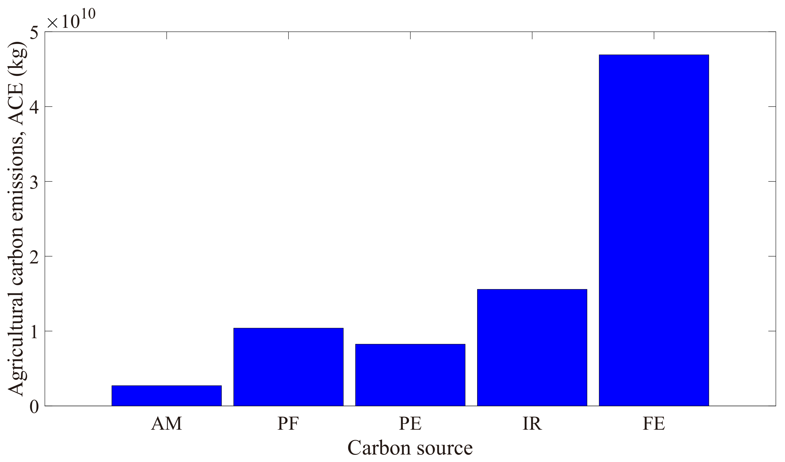
As we have discussed, there are five main sources of the agricultural carbon emission, which are the use of the agricultural machinery (AM), the production and use of agricultural plastic film (PF), the the production and use of pesticide (PE), the carbon emissions from the irrigation (IR) and the production and use of fertilizers (FE).

Figure 5 lists the quantities of the ACE of the five main sources in 2019. Consistent with our predictions, fertilizers is the majority source of the ACE which is approximately 56% of the total ACE. The proportions of the AM, PF, PE and IR are approximately 3%, 12%, 10% and 19%. In light of this, the main problem of reducing agricultural carbon emissions is to reduce the use of chemical fertilizers. One of the most acceptable approaches is to substitute chemical fertilizers by biological fertilizer. Biological fertilizer is also called organic fertilizer or bacterial manure which refers to the fertilizer produced by the decomposition of agricultural wastes such as crop straw. Although the decomposition of agricultural wastes will also produce carbon emissions, it is more efficient in the use of carbon element, and thus, it is cleaner compared with the produce of the chemical fertilizer.

In Figure 6, the regional levels of the ACE of each of the sources are given. For all of the five sources except PF, the ACE of the middle region is the highest and the ACE of the western region is the lowest. The ACE of PF of the middle region is not significantly higher than that of the other two regions. Given by the heights of the 15 bars in Figure 6, it also suggests that the effective way to reduce agricultural carbon emissions is to reduce the use of chemical fertilizers.

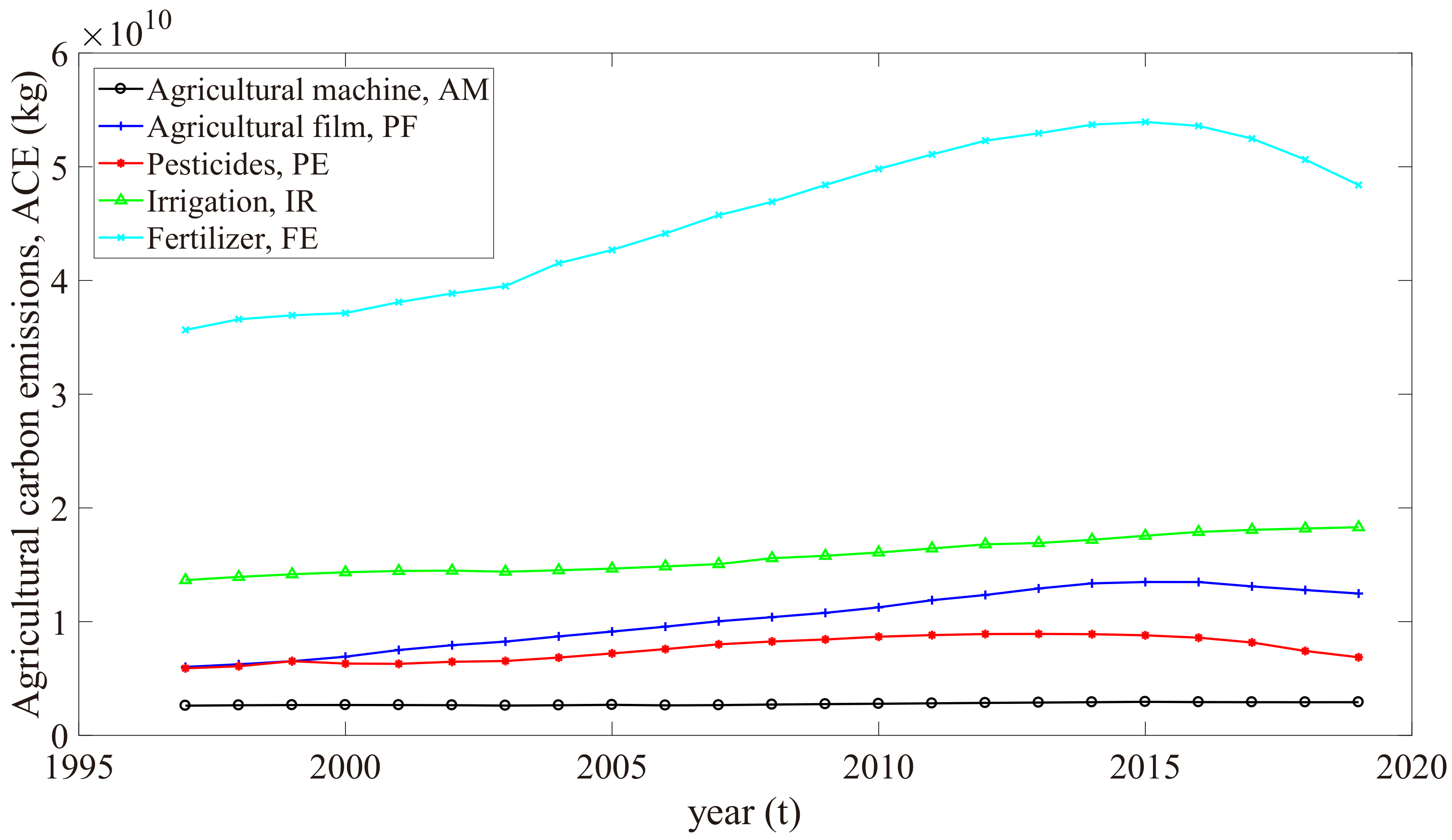
Beyond the regional difference, Figure 7 shows the historical trends of the five main sources of the ACE. First, the ACE of FE has a similar trend as the historical aggregate ACE, and the changes in the rest of the four sources are relatively small. The ACE of PF and PE also reflect up and down trends but, since they have relatively small proportions, the changes are not important for the ACE issue.

Until now, both the bad news and good news are very clear. The bad news is that the majority of the ACE is caused by the production and use of the chemical fertilizers. If we reduce the use of the chemical fertilizers directly, although the agricultural carbon emission should be significantly reduced, the agricultural output may be negatively affected. The good news is that the historical trend of the ACE of FE is already reduced in recent years. Evidence also supports that this reduction is not caused by the political target.

4.3. The Effect of the ACE on Economic Growth

We have discussed the way of reducing the agricultural carbon emission in previous contents. The quality of the environment is a necessary focus, but the economic cost also needs to be considered. In other words, the question becomes that, if agricultural carbon emission is really reduced, what are the consequences to the agricultural economy as well as the whole economy?

We firstly calculate the ratio of $ACE$ to $AGDP$ as an index, namely $ACEPY$ (=$ACE/AGDP)$, to show the “cleanliness” of agricultural production. A lower $ACEPY$ means higher degree of health of the agricultural economy, and a higher $ACEPY$ means a lower degree of health of the agricultural economy. The $ACEPY$ index of the year 2019 is standardized and is shown in Figure 8. Deep red means healthy and light red means unhealthy agricultural economy.

Figure 8 shows a very significant feature that the south is generally healthier than the north. Given by the three regions (eastern, middle and western) defined in Figure 1, it seems that the agricultural industry is relatively healthy in the eastern region and is relatively unhealthy is the western region, but this feature is not quite obvious. One of the most possible reasons is that the agricultural industry in northern China is underdeveloped. No matter where this comes from, an intuitive suggestion is that if the scale of agriculture will inevitably expand, it is better to develop more agricultural industries in southern rather than northern China.

According to the methods discussed in Section 3.3, we will now quantitatively exam the inverted “U”-shape effect of $ACE$ on economic growth. Given the panel data of the 31 provinces from 2000 to 2019, all the the pooled OLS models, fixed effect (FE) models and random effects (RE) models are employed for both of the empirical Equations (7) and (8). The individual effect is assumed to be none in the pooled OLS model, is assumed to be correlated with explanatory variables in the FE model and is assumed to be uncorrelated with explanatory variables in the RE model. A Hausman test can be used to check the empirical status of the individual effect. In other words, the results of the Hausman test can tell us the most appropriate model among the three models. The Hausman test statistics between FE estimators and RE estimators of both Equations (7) and (8) are <0.0001. Thus, FE estimators are more appropriate to describe the empirical relations. The Hausman test statistics between FE estimators and pooled OLS estimators of both Equations (7) and (8) are <0.0001. Thus, FE estimators are more appropriate to describe the empirical relations. However, the FE model has a problem in that it cannot estimate the effect of the time-invariant explanatory variable on the dependent variable, and the results of the pooled OLS are also shown as comparisons. The regression results are summarized in

Table 4. Estimated Results of the agricultural GDP.

Number:	Reg.(1)	Reg.(2)	Reg.(3)
Model:	Pooled OLS	FE	RE
Dependent:	ln($\mathit{AGDP}$)	ln($\mathit{AGDP}$)	ln($\mathit{AGDP}$)
ln($POP$)	0.410 ***	2.925 ***	0.265 **
	(0.053)	(0.176)	(0.106)
ln($SIZE$)	0.017		−0.139 **
	(0.023)		(0.068)
$ACE$	7.67 $\times {10}^{-10}$ ***	1.31 $\times {10}^{-9}$ ***	1.15 $\times {10}^{-9}$ ***
	(5.51 $\times {10}^{-11}$)	(6.04 $\times {10}^{-11}$)	(7.35 $\times {10}^{-11}$)
$AC{E}^2$	−5.88 $\times {10}^{-20}$ ***	−6.53 $\times {10}^{-20}$ ***	−6.39 $\times {10}^{-20}$ ***
	(5.24 $\times {10}^{-20}$)	(6.24 $\times {10}^{-21}$)	(7.47 $\times {10}^{-21}$)
$constant$	1.711 ***	−19.826 ***	3.771 ***
	(0.541)	(1.405)	(1.194)
Obs.	620	620	620
$R^2$ (within)	0.799	0.708	0.598
Hausman test			<0.001

Notes: |t| in parentheses; *, **, and *** are significant at the 10%, 5% and 1% levels.

and

Table 5. Estimated Results of the GDP.

Number:	Reg.(4)	Reg.(5)	Reg.(6)
Model:	Pooled OLS	FE	RE
Dependent:	ln($\mathit{GDP}$)	ln($\mathit{GDP}$)	ln($\mathit{GDP}$)
ln($POP$)	0.793 ***	5.689 ***	0.364 **
	(0.076)	(0.242)	(0.145)
ln($SIZE$)	−0.320 ***		−0.577 ***
	(0.033)		(0.085)
$ACE$	2.82 $\times {10}^{-10}$ ***	1.45 $\times {10}^{-9}$ ***	1.03 $\times {10}^{-9}$ ***
	(7.88 $\times {10}^{-11}$)	(8.32 $\times {10}^{-11}$)	(1.15 $\times {10}^{-10}$)
$AC{E}^2$	−1.91 $\times {10}^{-20}$ **	−6.44 $\times {10}^{-20}$ ***	−5.36 $\times {10}^{-20}$ ***
	(7.48 $\times {10}^{-21}$)	(8.64 $\times {10}^{-21}$)	(1.16 $\times {10}^{-20}$)
$constant$	5.823 ***	−40.235 ***	10.764 ***
	(0.773)	(1.935)	(1.586)
Obs.	620	620	620
$R^2$ (within)	0.616	0.716	0.505
Hausman test			<0.001

Notes: |t| in parentheses; *, **, and *** are significant at the 10%, 5% and 1% levels.

.

The results in Table 4 and Table 5 have many implications. First, in general, the relatively higher $R^2$ implies the high reliability of the regression. The $R^2$ of Reg.(2) is quite close to that of Reg.(5). This implies that the $ACE$ values have similar explanatory power to $AGDP$ and $GDP$. Second, because the size of the provinces is time invariant, this kind of time-invariant variable will be removed in the FE model due to the estimation method of taking difference, and the influence of ln$SIZE$ on dependents cannot be estimated by the FE model. Although not shown in the table, the results of the Hausman test point out that the FE model is better than the pooled OLS model in describing both Equations (7) and (8) under a 0.05 significance level. In other words, Reg.(2) is better than Reg.(1) and Reg.(5) is better than Reg.(4). Third, all the estimators of $ACE$ and $AC{E}^2$ are significant, the estimators of $ACE$ are positive, and the estimators of $AC{E}^2$ are negative. These imply the inverted “U”-shape relations of $ACE$ on both $AGDP$ and $GDP$. The peak of the parabola can be calculated by equation $AC{E}^p=-0.5\times b_3/b_4$ where $b_3$ is the estimator of $ACE$ and $b_4$ is the estimator of $AC{E}^2$. Reg.(2) implies that the peak is $1.003\times {10}^{10}$ (kg) ACE for agricultural GDP, and Reg.(5) implies that the peak is $1.256\times {10}^{10}$ (kg) ACE for GDP. According to the data of the provincial ACE in 2019, the average provincial level of ACE is $2.87\times {10}^9$ (kg). The highest and lowest amount of the ACE are $9.23\times {10}^9$ (kg) at Henan and $1.37\times {10}^8$ (kg) at Tibet. Practically, the current ACE values of all the provinces are lower than the two turning points. In other words, now, more ACE still implies more agricultural output. This result is understandable, since the agricultural industry and especially the planting industry has higher tolerance than humans do. For example, a high concentration of carbon dioxide is helpful for plant growth. Therefore, for the issue of carbon emission, we would like a world with lower carbon emission, but this will negatively affect the agricultural economy.

5. Conclusions

This study aims to describe and analyze the time trend and spatial distribution of the agricultural carbon emission of China. Estimation methods of the five main sources of the agricultural carbon emission are introduced. Given the panel data of the 31 provinces from 1996 to 2019, the time trend and spatial distribution are empirically discussed. Furthermore, for the purpose of exploring the effect of agricultural carbon emission on economic growth, theoretical and empirical works are also provided. Results show that (i) the carbon emission started to fall after 2015, and thus, the future situation should be more optimistic; (ii) the majority source of the carbon emission is caused by the production and use of the chemical fertilizer, which is approximately half in total; (iii) the agricultural carbon emission has a significant inverted “U”-shape effect on both the agricultural GDP and GDP controlling for all other variables, and current provincial ACE levels are obviously smaller than the turning points of the two.

Corresponding with all the findings in this study, we have three suggestions. First, we should continue to make ACE decline steadily and naturally with the natural development of the economy and society. Second, local governments should formulate carbon emission policies according to their particular local agricultural conditions and carbon source characteristics. Third, the government must accept a trade-off between economic development, especially the agricultural economic development, and the quality of the natural environment. We can neither give up development in order to protect the environment nor emit a large amount of carbon for development.

There are a couple of limitations in this study. We have found that the agricultural carbon emission fell in recent years, and this is caused by the fall in the production and the use of the chemical fertilizer. It is necessary to continuously explore the determinants of the fall. If so, a more targeted policies suggestion can be given. Another issue in this study is that we only analyze the effect of ACE on economic growth, but they affect each other. Next, we decide to explore this issue by, for example, a Panel VAR model in the future.