Figure 1.
Map of Senegal with its ten data source locations (at left).
Figure 1.
Map of Senegal with its ten data source locations (at left).
Figure 2.
Map of Senegal showing locations for exploratory data analysis.
Figure 2.
Map of Senegal showing locations for exploratory data analysis.
Figure 3.
Annual cumulative rainfall variation for Matam, Kaolack and Kolda (1982–2020).
Figure 3.
Annual cumulative rainfall variation for Matam, Kaolack and Kolda (1982–2020).
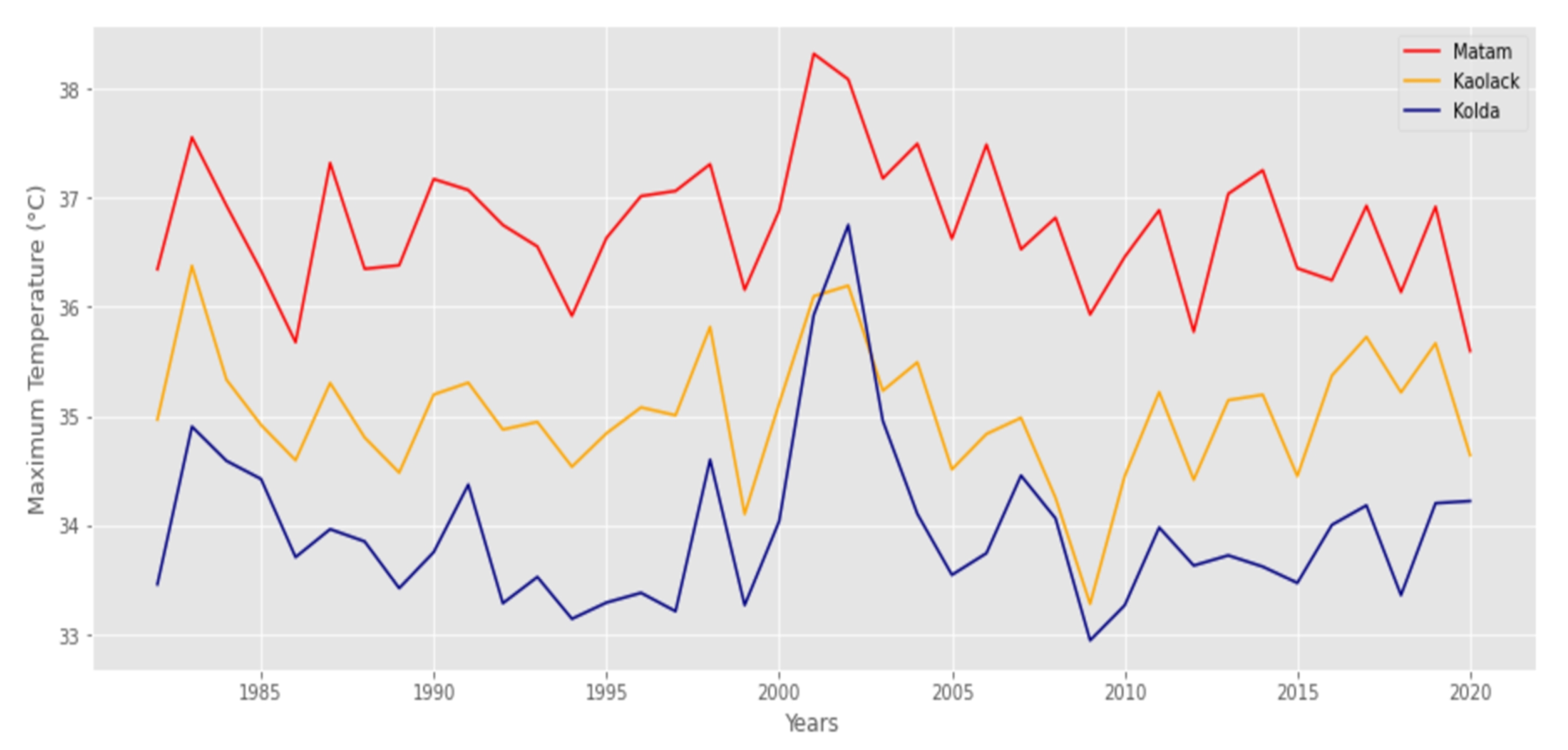
Figure 4.
Annual average Maximum Temperature for Matam, Kaolack and Kolda (1982–2020).
Figure 4.
Annual average Maximum Temperature for Matam, Kaolack and Kolda (1982–2020).
Figure 5.
Annual average Minimum Temperature for Matam, Kaolack and Kolda (1982–2020).
Figure 5.
Annual average Minimum Temperature for Matam, Kaolack and Kolda (1982–2020).
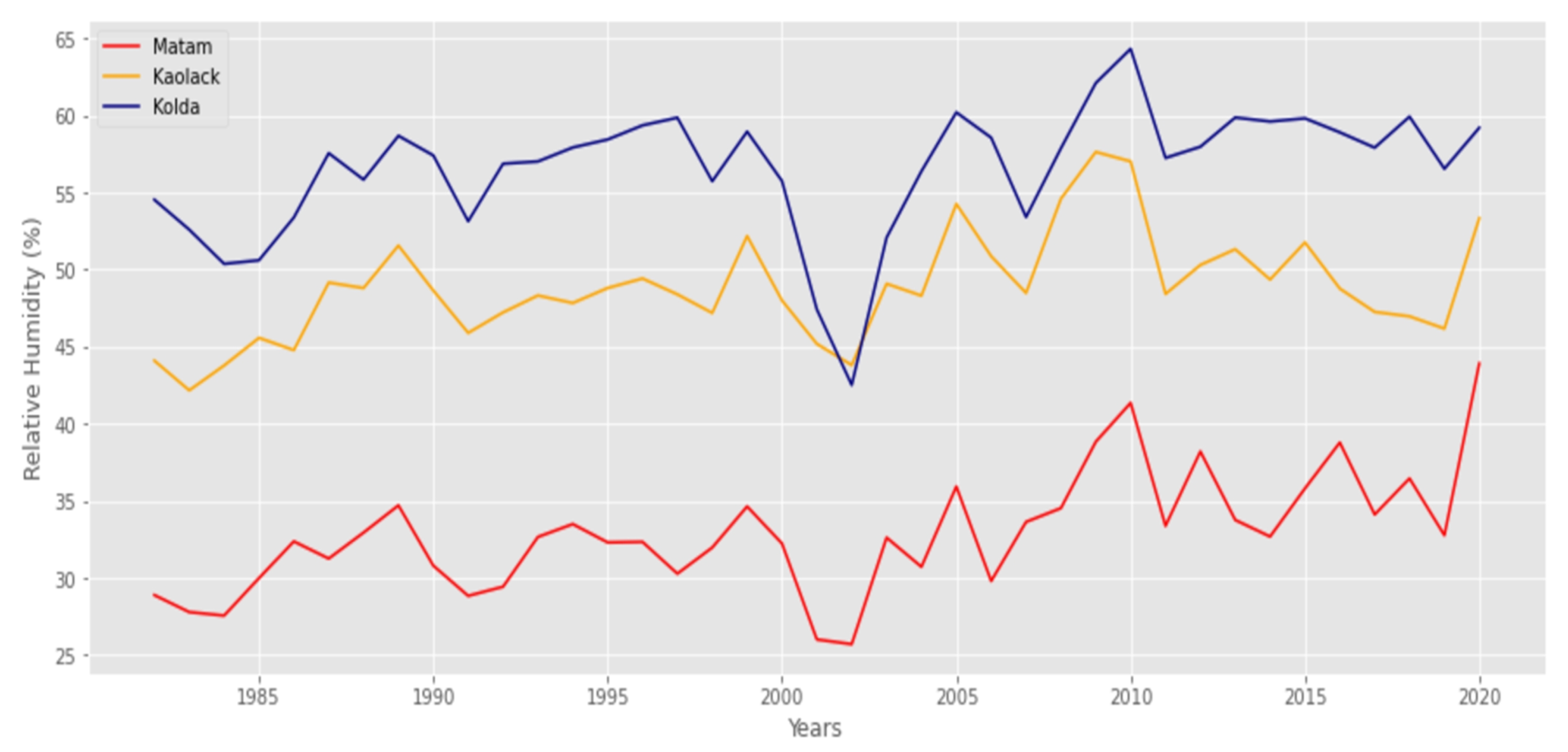
Figure 6.
Annual average Relative Humidity for Matam, Kaolack and Kolda (1982–2020).
Figure 6.
Annual average Relative Humidity for Matam, Kaolack and Kolda (1982–2020).
Figure 7.
Monthly average rainfall variation for Matam, Kaolack and Kolda (1982–2020).
Figure 7.
Monthly average rainfall variation for Matam, Kaolack and Kolda (1982–2020).
Figure 8.
Monthly average Maximum Temperature for Matam, Kaolack and Kolda (1982–2020).
Figure 8.
Monthly average Maximum Temperature for Matam, Kaolack and Kolda (1982–2020).
Figure 9.
Monthly average Minimum Temperature for Matam, Kaolack and Kolda (1982–2020).
Figure 9.
Monthly average Minimum Temperature for Matam, Kaolack and Kolda (1982–2020).
Figure 10.
Monthly average Relative Humidity for Matam, Kaolack and Kolda (1982–2020).
Figure 10.
Monthly average Relative Humidity for Matam, Kaolack and Kolda (1982–2020).
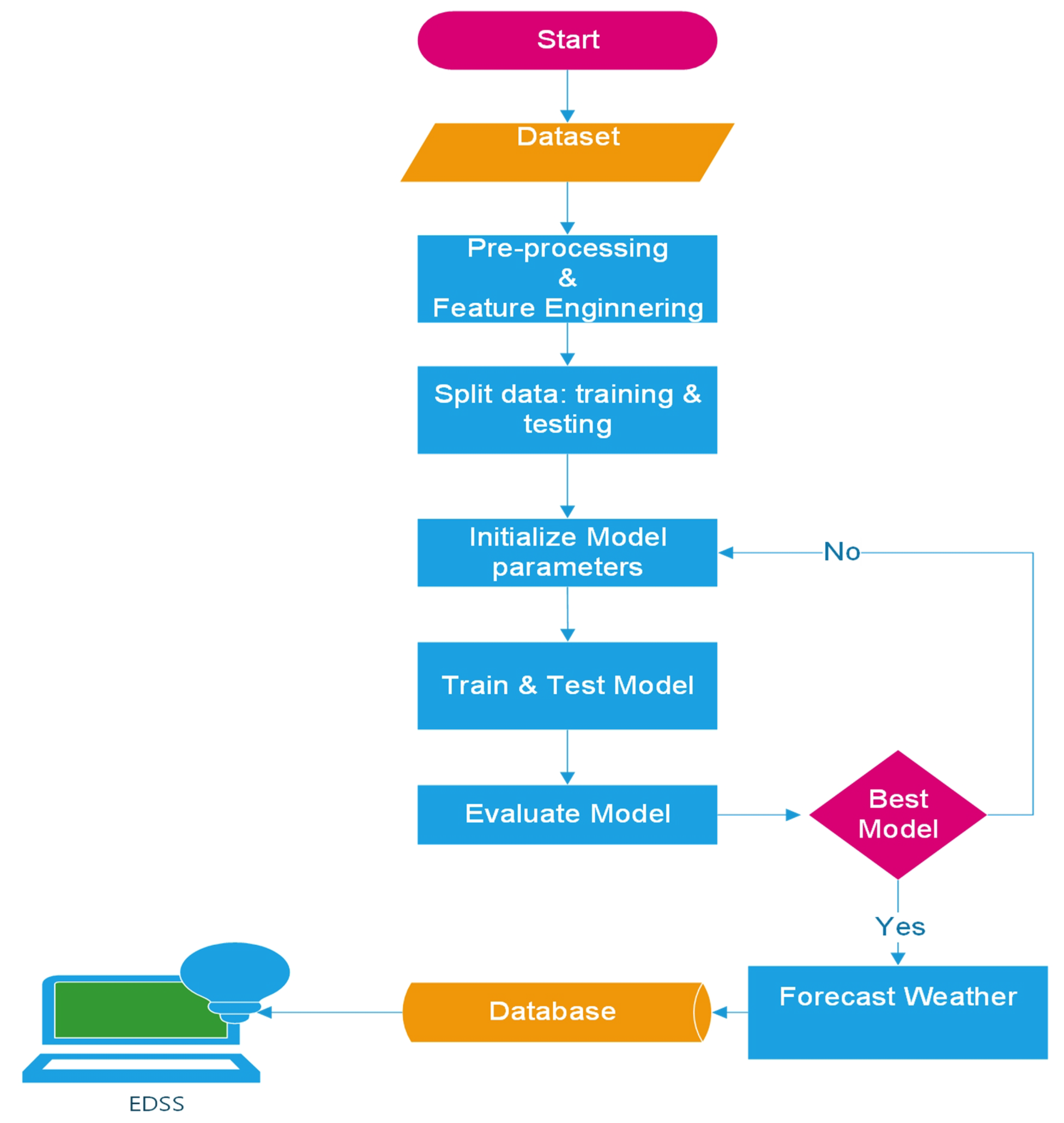
Figure 11.
Flowchart summarizing the entire study.
Figure 11.
Flowchart summarizing the entire study.
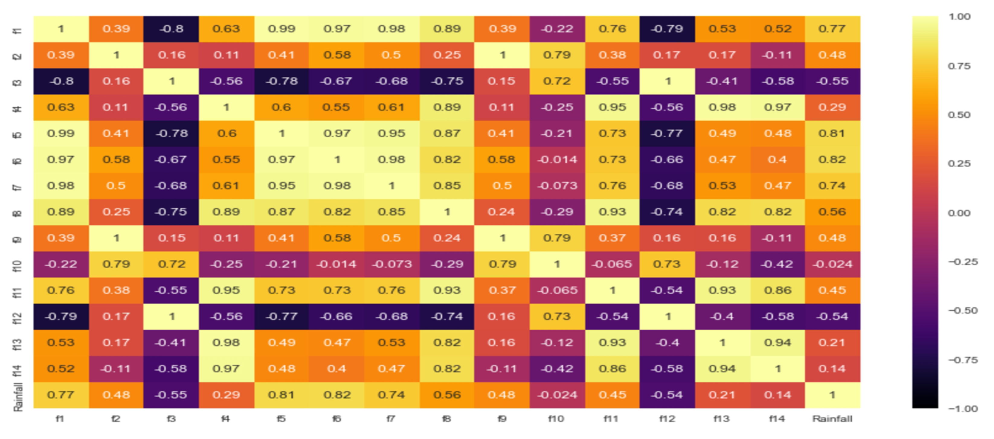
Figure 12.
Correlation summary for Rainfall, Relative Humidity, Maximum Temperature, Minimum Temperature and Day of Year.
Figure 12.
Correlation summary for Rainfall, Relative Humidity, Maximum Temperature, Minimum Temperature and Day of Year.
Figure 13.
Autocorrelation summary for Relative Humidity, Maximum Temperature, Minimum Temperature and Rainfall.
Figure 13.
Autocorrelation summary for Relative Humidity, Maximum Temperature, Minimum Temperature and Rainfall.
Figure 14.
Correlation of features after feature engineering and data transformation.
Figure 14.
Correlation of features after feature engineering and data transformation.
Figure 15.
Summary of sliding window with one-step forecasting technique.
Figure 15.
Summary of sliding window with one-step forecasting technique.
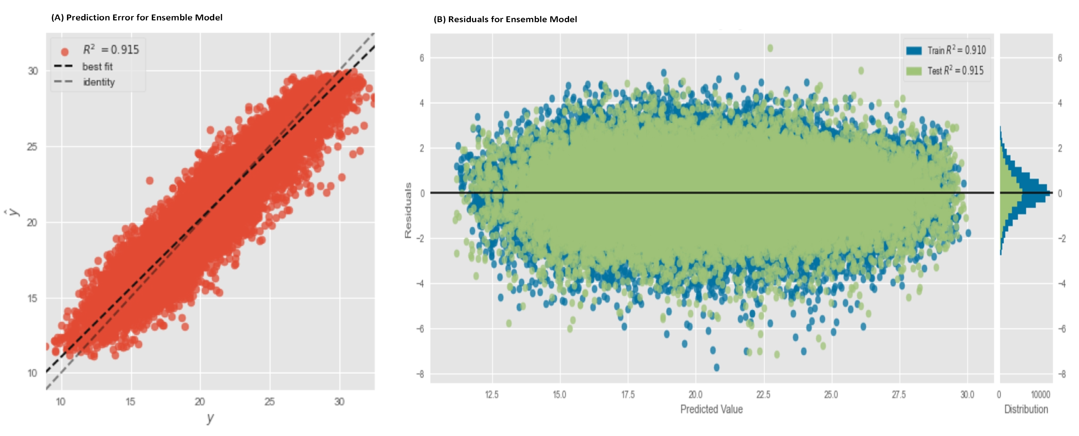
Figure 16.
Accuracy of Ensemble Model for Relative Humidity forecasting.
Figure 16.
Accuracy of Ensemble Model for Relative Humidity forecasting.
Figure 17.
Accuracy of Ensemble Model for Minimum Temperature forecasting.
Figure 17.
Accuracy of Ensemble Model for Minimum Temperature forecasting.
Figure 18.
Accuracy of Ensemble Model for Maximum Temperature forecasting.
Figure 18.
Accuracy of Ensemble Model for Maximum Temperature forecasting.
Figure 19.
Accuracy of Ensemble Model for Rainfall forecasting.
Figure 19.
Accuracy of Ensemble Model for Rainfall forecasting.
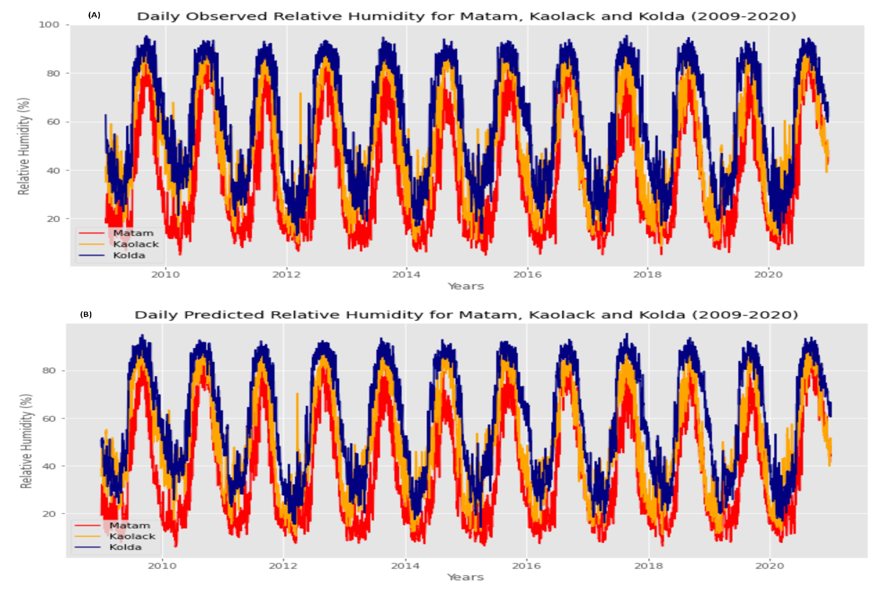
Figure 20.
Observed and Forecasted Relative Humidity for Matam, Kaolack and Kolda (2009–2020).
Figure 20.
Observed and Forecasted Relative Humidity for Matam, Kaolack and Kolda (2009–2020).
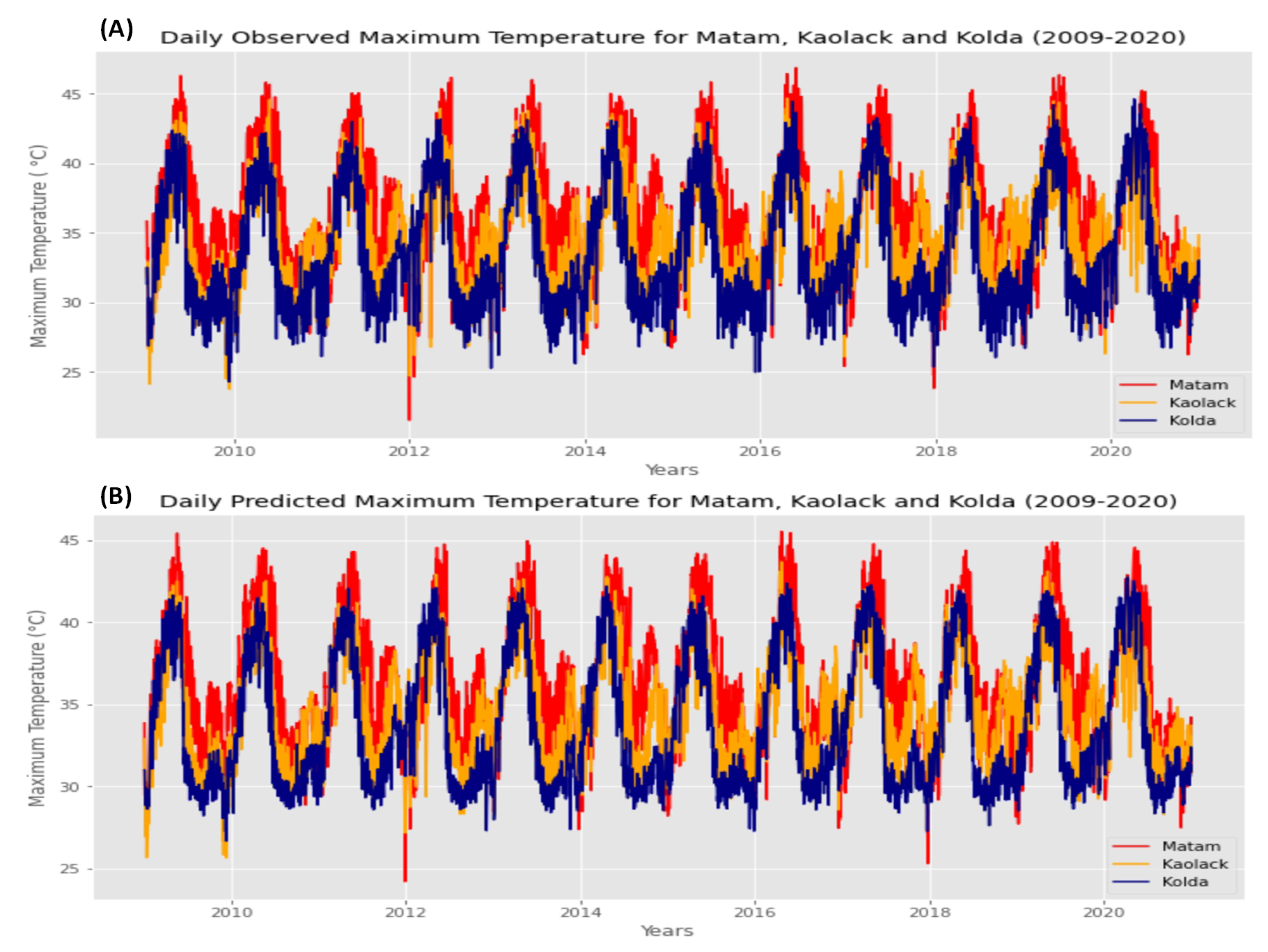
Figure 21.
Observed and Forecasted Maximum Temperature for Matam, Kaolack and Kolda (2009–2020).
Figure 21.
Observed and Forecasted Maximum Temperature for Matam, Kaolack and Kolda (2009–2020).
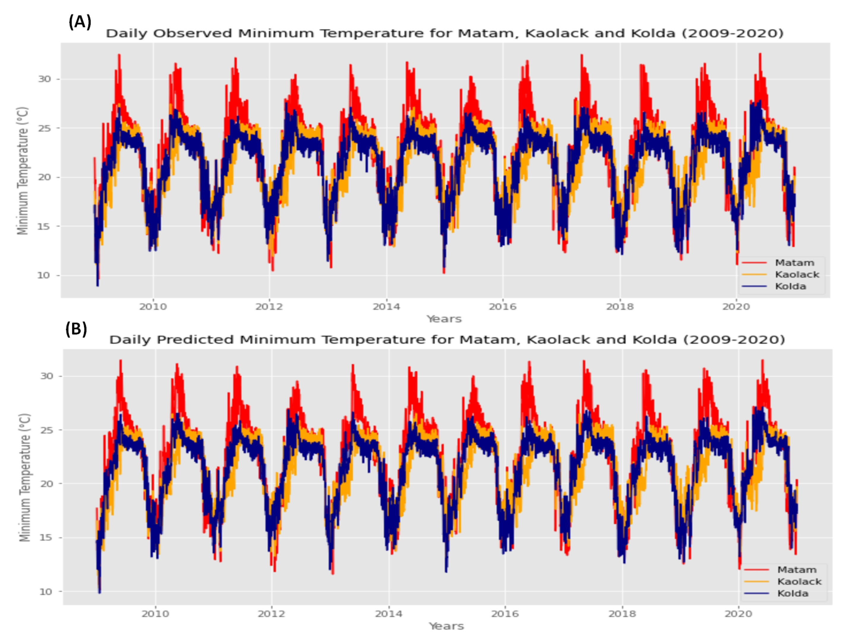
Figure 22.
Observed and Forecasted Minimum Temperature for Matam, Kaolack and Kolda (2009–2020).
Figure 22.
Observed and Forecasted Minimum Temperature for Matam, Kaolack and Kolda (2009–2020).
Figure 23.
Observed and Forecasted Rainfall for Matam, Kaolack and Kolda (2009–2020).
Figure 23.
Observed and Forecasted Rainfall for Matam, Kaolack and Kolda (2009–2020).
Figure 24.
Monthly Average Observed and Forecasted Relative Humidity for Matam, Kaolack and Kolda (2009–2020).
Figure 24.
Monthly Average Observed and Forecasted Relative Humidity for Matam, Kaolack and Kolda (2009–2020).
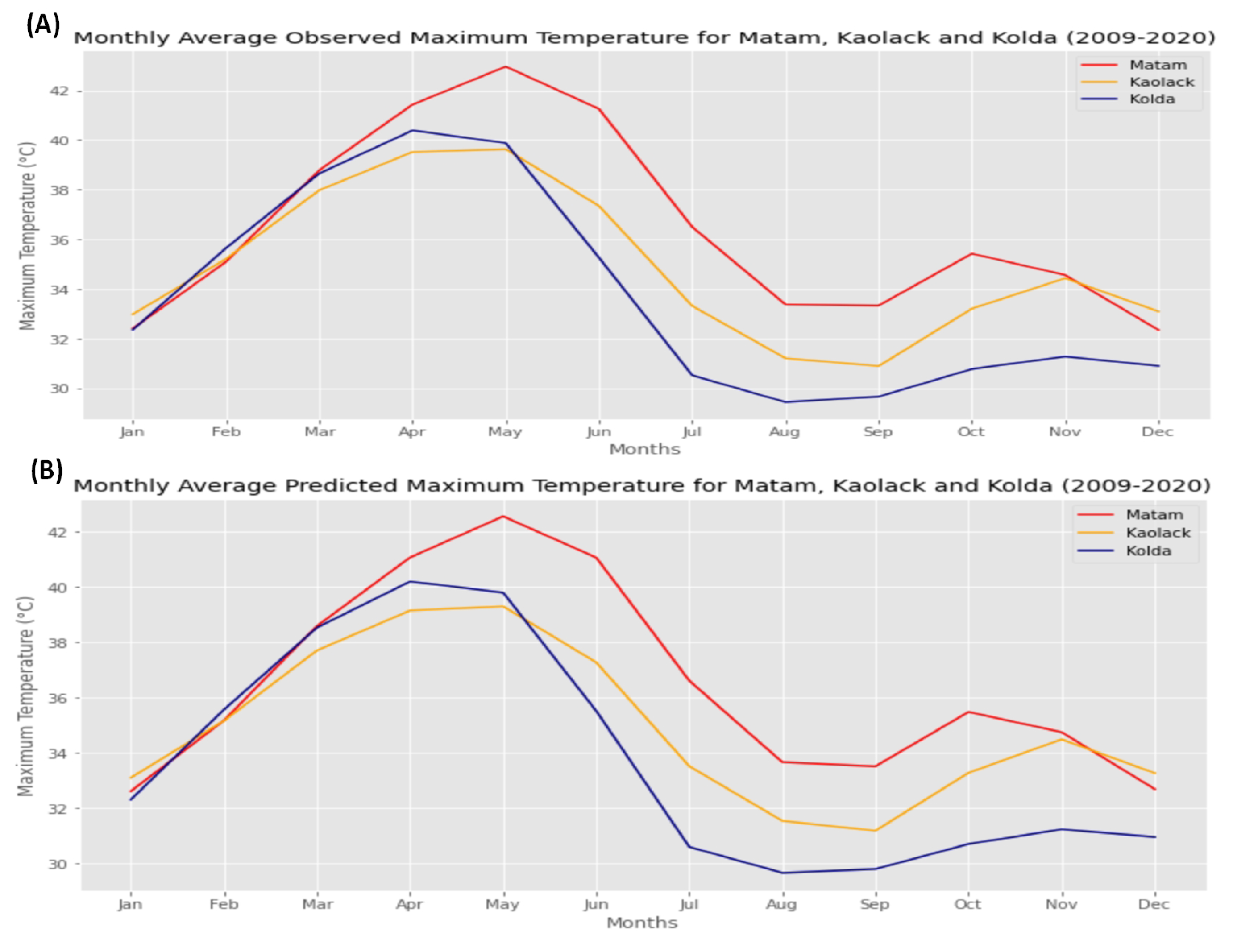
Figure 25.
Monthly Average Observed and Forecasted Maximum Temperature for Matam, Kaolack and Kolda (2009–2020).
Figure 25.
Monthly Average Observed and Forecasted Maximum Temperature for Matam, Kaolack and Kolda (2009–2020).
Figure 26.
Monthly Average Observed and Forecasted Minimum Temperature for Matam, Kaolack and Kolda (2009–2020).
Figure 26.
Monthly Average Observed and Forecasted Minimum Temperature for Matam, Kaolack and Kolda (2009–2020).
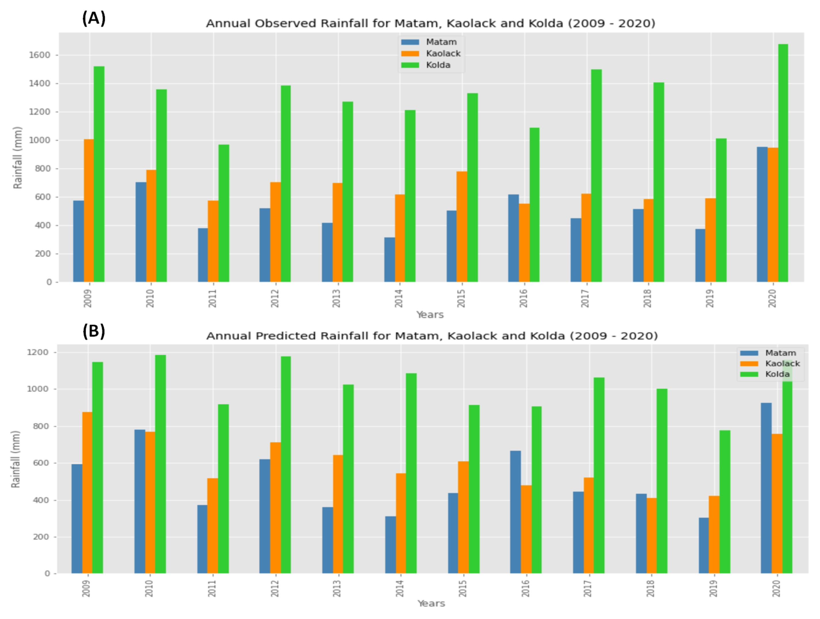
Figure 27.
Monthly Average Observed and Forecasted Rainfall for Matam, Kaolack and Kolda (2009–2020).
Figure 27.
Monthly Average Observed and Forecasted Rainfall for Matam, Kaolack and Kolda (2009–2020).
Table 1.
Summary of Latitude and Longitude of selected locations.
Table 1.
Summary of Latitude and Longitude of selected locations.
| Station | Latitude | Longitude |
|---|
| Rosso | 16.5 N | −15.817 W |
| Saint-Louis | 16.05 N | −16.483 W |
| Cap-skiring | 12.4 N | −16.75 W |
| Diourbel | 14.65 N | −16.233 W |
| Kaolack | 14.133 N | −16.067 W |
| Kedougou | 12.567 N | −12.217 W |
| Kolda | 12.883 N | −14.967 W |
| Linguere | 15.367 N | −15.117 W |
| Matam | 15.617 N | −13.25 W |
| Tambacounda | 13.767 N | −13.683 W |
Table 2.
Model performance for Relative Humidity Forecasting.
Table 2.
Model performance for Relative Humidity Forecasting.
| Model | MAE | MSE | RMSE | |
|---|
| Ensemble Model | 4.0126 | 29.9885 | 5.4428 | 0.9335 |
| Light Gradient Boosting Machine | 4.0693 | 30.6936 | 5.5040 | 0.9317 |
| CatBoost Regressor | 4.0619 | 30.7052 | 5.5046 | 0.9317 |
| Gradient Boosting Regressor | 4.0863 | 30.8061 | 5.5140 | 0.9314 |
| Extreme Gradient Boosting | 4.1601 | 32.1831 | 5.6292 | 0.9280 |
| Random Forest Regressor | 4.2284 | 32.9041 | 5.7005 | 0.9270 |
| Orthogonal Matching Pursuit | 4.2385 | 33.1158 | 5.7223 | 0.9268 |
| Extra Trees Regressor | 4.2533 | 33.3111 | 5.7349 | 0.9260 |
| K Neighbors Regressor | 4.4810 | 36.5971 | 6.0138 | 0.9184 |
| AdaBoost Regressor | 5.7023 | 48.4746 | 6.9384 | 0.8954 |
| Decision Tree Regressor | 5.9400 | 65.2236 | 8.0390 | 0.8553 |
Table 3.
Model performance for Minimum Temperature Forecasting.
Table 3.
Model performance for Minimum Temperature Forecasting.
| Model | MAE | MSE | RMSE | |
|---|
| Ensemble Model | 0.7908 | 1.1329 | 1.0515 | 0.9018 |
| Gradient Boosting Regressor | 0.7953 | 1.1481 | 1.0582 | 0.9006 |
| Light Gradient Boosting Machine | 0.7966 | 1.1508 | 1.0595 | 0.9004 |
| CatBoost Regressor | 0.7983 | 1.1554 | 1.0614 | 0.9001 |
| Extreme Gradient Boosting | 0.8107 | 1.1893 | 1.0771 | 0.8971 |
| Orthogonal Matching Pursuit | 0.8199 | 1.2034 | 1.0840 | 0.8956 |
| Random Forest Regressor | 0.8248 | 1.2200 | 1.0922 | 0.8942 |
| Extra Trees Regressor | 0.8301 | 1.2326 | 1.0982 | 0.8931 |
| K Neighbors Regressor | 0.8793 | 1.3646 | 1.1573 | 0.8815 |
| AdaBoost Regressor | 0.8961 | 1.4137 | 1.1727 | 0.8787 |
| Decision Tree Regressor | 1.1877 | 2.4335 | 1.5515 | 0.7865 |
Table 4.
Model performance for Maximum Temperature Forecasting.
Table 4.
Model performance for Maximum Temperature Forecasting.
| Model | MAE | MSE | RMSE | |
|---|
| Ensemble Model | 1.2515 | 2.8038 | 1.6591 | 0.8205 |
| Light Gradient Boosting Machine | 1.2618 | 2.8418 | 1.6694 | 0.8176 |
| Gradient Boosting Regressor | 1.2678 | 2.8478 | 1.6725 | 0.8175 |
| CatBoost Regressor | 1.2624 | 2.8501 | 1.6716 | 0.8171 |
| Extreme Gradient Boosting | 1.2878 | 2.9636 | 1.7031 | 0.8095 |
| Random Forest Regressor | 1.3031 | 3.0114 | 1.7195 | 0.8071 |
| Extra Trees Regressor | 1.3116 | 3.0473 | 1.7298 | 0.8048 |
| Orthogonal Matching Pursuit | 1.3240 | 3.1079 | 1.7519 | 0.8016 |
| K Neighbors Regressor | 1.3811 | 3.3403 | 1.8128 | 0.7865 |
| AdaBoost Regressor | 1.4331 | 3.3870 | 1.8281 | 0.7841 |
| Decision Tree Regressor | 1.8775 | 6.1235 | 2.4593 | 0.6098 |
Table 5.
Model performance for Rainfall Forecasting.
Table 5.
Model performance for Rainfall Forecasting.
| Model | MAE | MSE | RMSE | |
|---|
| Ensemble Model | 0.2142 | 0.1681 | 0.4100 | 0.7733 |
| CatBoost Regressor | 0.2150 | 0.1691 | 0.4112 | 0.7719 |
| Light Gradient Boosting Machine | 0.2146 | 0.1695 | 0.4117 | 0.7714 |
| Gradient Boosting Regressor | 0.2221 | 0.1752 | 0.4185 | 0.7638 |
| Extreme Gradient Boosting | 0.2178 | 0.1752 | 0.4185 | 0.7638 |
| Random Forest Regressor | 0.2212 | 0.1797 | 0.4238 | 0.7578 |
| Extra Trees Regressor | 0.2246 | 0.1851 | 0.4302 | 0.7504 |
| K Neighbors Regressor | 0.2316 | 0.2022 | 0.4496 | 0.7272 |
| AdaBoost Regressor | 0.3803 | 0.2851 | 0.5325 | 0.6147 |
| Orthogonal Matching Pursuit | 0.4127 | 0.3336 | 0.5775 | 0.5502 |
| Decision Tree Regressor | 0.2910 | 0.3452 | 0.5875 | 0.5343 |
Table 6.
Summary of our results and results from other studies.
Table 6.
Summary of our results and results from other studies.
| Authors | Model | Parameter | MAE | RMSE |
|---|
| Our results | | Relative Humidity | 0.1873 | 0.1369 |
| Ensemble Model | Minimum Temperature | 0.1881 | 0.1429 |
| | Maximum Temperature | 0.1898 | 0.144 |
| | Rainfall | 0.2987 | 0.1787 |
| [20] | Random Forest | | 4.49 | 8.82 |
| Multivariate Linear Regression | Rainfall | 4.97 | 8.61 |
| XGBoost | | 3.58 | 7.85 |
| [33] | XGBoost | Rainfall | 8.8 | 2.7 |
| [34] | Linear Regression | Maximum Temperature | 3.10 | 1.78 |
| [35] | | Indoor Air Temperature | 0.3535 | 0.476 |
| Random Forest | Indoor Relative Humidity | 1.47 | 2.429 |


