Prediction of Corn Yield in the USA Corn Belt Using Satellite Data and Machine Learning: From an Evapotranspiration Perspective

Abstract

The reliable prediction of corn yield for the United States of America is essential for effective food and energy management of the world. Three satellite-derived variables were selected, namely enhanced vegetation index (EVI), leaf area index (LAI) and land surface temperature (LST). The least absolute shrinkage and selection operator (LASSO) was used for regression, while random forest (RF), support vector regression (SVR) and long short-term memory (LSTM) methods were selected for machine learning. The three variables serve as inputs to these methods, and their efficacy in predicting corn yield was assessed in relation to evapotranspiration (ET). The results confirmed that a high level of performance can be achieved for yield prediction (mean predicted R² = 0.63) by combining EVI + LAI + LST with the four methods. Among them, the best results were obtained by using LSTM (mean predicted R² = 0.67). EVI and LST provided extra and unique information in peak and early growth stages for corn yield, respectively, and the usefulness of including LAI was not readily apparent across the whole season, which was consistent with the field growing conditions affecting the ET of corn. The satellite-derived data and the methods used in this study could be used for predicting the yields of other crops in different regions.

1. Introduction

The global food supply chain is facing increasing pressure from sustained population growth, climate change and changes in economic structure [1]. The prediction of crop yield at a regional scale is an important topic in agricultural studies, which can aid the government in evaluating the demand and supply of domestic agricultural products [2], and also help farmers make informed management and financial decisions [3]. As food, feed, an industrial grain crop and the third most important cereal crop worldwide after rice and wheat, corn is easy to process, readily digested and costs less to produce than other cereals, occupying an important position in the world economy. The United States of America (USA) was the largest corn producer in the world with an annual production of 0.366 billion metric tons in the 2018–2019 growing season (GS). Thus, the timely, convenient and reliable prediction of corn yield in the USA is of great significance for both regional and global food security.

Satellite remote sensing is an effective tool for predicting crop yields at large scales by monitoring crop growing conditions and growth environments [4,5]. Thus, satellite-derived data can be divided into data related to growing conditions, such as vegetation indices, photosynthetic activities [6,7], and phenology [8,9,10], and data related to growth environments, such as heat [11] and water stress [12,13]. Capturing crop growing conditions by use of spectral reflectance characteristics, the enhanced vegetation index (EVI) is the most widely used and classic vegetation index, which has been considered to be less sensitive to the background effects of the atmosphere and soil than the normalized difference vegetation index (NDVI) [14]. Defined as the one-sided green leaf area per unit ground area for broadleaf canopies, leaf area index (LAI) can be used for measuring the quantity and quality of canopy cover, which in turn has been related to plant physiological processes, such as photosynthesis and transpiration [15]. Providing a measure of plant heat stress, land surface temperature (LST) has also been widely accepted as an indicator of water stress in field crops [16]. Canopy temperature is directly associated with transpiration. Leaves cool down when the plant transpires and evaporates water. The cooling of leaves during evapotranspiration (ET) will then lower the surface temperature of the canopy. If moisture is restricted and transpiration is reduced, leaves will absorb radiation, leading to a rise in the surface temperature of the canopy. With the advancement of research, investigators have tried to use the complementary nature of EVI and LST [17,18,19] or EVI and LAI [20] in combination to predict crop yield. However, a limited number of studies have used all three variables in combination for analytical purposes.

As the satellite-derived data are sometimes affected by the same abiotic factors, or inter-related with each other, interpretation can be difficult. For example, the effects of temperature and soil moisture on evapotranspiration (ET) are mediated by plant leaves (LAI) [21], with LAI, in turn, sensitive to changes in EVI [22]. LAI also affects soil temperature, air temperature, relative humidity and the microclimate of the plant canopy. In fact, it is not clear how the information from the three satellite-derived indices singularly and interactively confounds the interpretation of the final corn yield at a large scale. Some studies have explored the roles of satellite-based growing conditions and environment monitoring data in relation to the prediction of crop yields. However, the existing studies based on the combined application of two satellite-derived indices (i.e., paired indices) did not explain the relationship between these data; more specifically, why these data can be combined and the associated crop growth principles involved.

Here, it was hypothesized that EVI, LAI and LST make both unique and shared contributions to the prediction of yield from an ET perspective. Closely related to crop yield, ET is an important metric for studying the relationship between crop yield and water content and represents the production capacity of crops [23], which can be regarded as the result of the comprehensive impact of many key environmental factors on crops [24]. As an important link for water movement in the soil–plant–atmosphere system, ET is mainly affected by soil moisture in the soil system, crop leaf conditions in the crop system as well as solar radiation in the atmospheric system. Scholars analyzed the factors influencing actual ET in addition to soil moisture (monitored by temperature vegetation dryness index, TVDI) and solar radiation [23]. Soil moisture represents the soil system, while solar radiation represents the atmospheric system, which simply simulates the soil–atmosphere system to estimate crop yield. However, the water movement of crops involves a continuous system of soil–crop–atmosphere. In order to explain the effect of water stress on crop yield from an ET perspective, consideration should be given to all three components of the soil–crop–atmosphere system. In the crop system, crop coverage and the number of leaf stomata also have an impact on ET. Larger coverage means more exposure of leaves to light, causing increased stomatal density (number of stomata per unit of area) and stomatal index (ratio of stomata to epidermal cells plus stomata), which enhance the intensity of water exercise [25]. LAI can describe the degree of canopy coverage, which provides a measure of foliage density and has been closely linked to the photosynthetic and ET capacities of plants [26,27]. TVDI based on the relationship between EVI and LST can be used to indirectly assess crop water stress [28]. Nevertheless, simulating dry/wet edges to calculate TVDI is probably problematic, as satellite images are lacking in sufficient pixels to identify the dryness and wetness extremes of different coverages [29]. Hence, EVI and LST should be used separately to represent soil moisture. As satellite data can dynamically capture crop growing conditions and environments when used singly or in combination, the three satellite-derived indices were selected as the surrogate indicators of plant–soil water relations and, hence, crop ET. In the case that they have commonly shared and complementary information to contribute to the prediction of yield, the focus was also put on determining their contributions to the prediction of corn yield in the USA.

Methods of crop yield prediction can be summarized as empirical and process-based models [19] that both have their pros and cons and can achieve good prediction. The rapid development of remote sensing techniques greatly benefits empirical models [30,31,32,33] which include statistical regression and machine learning (ML). Compared with the process-based model, empirical models provide a simpler alternative to spatially explicit studies and have the advantages of simplicity, fewer inputs required and relatively high prediction power in the case of sufficient training data [19]. Support vector regression (SVR), random forest (RF), neural networks (NN) and other ML methods have demonstrated their powering performance in the prediction or estimation of crop yield [33,34,35,36]. Different from conventional regression models, ML methods are capable of deep mining features and can capture nonlinear relationships between prediction or estimation variables and crop yield [19,33,36,37]. Called long short-term memory (LSTM), a specific variation of NN has been more recently noticed in yield prediction due to its large capacity to cope with sequential data [17].

In this study, EVI, LAI and LST were utilized to build statistical models using three ML methods and a linear regression (LR) method based on influencing factors for ET. The three ML methods used for this purpose were SVR, RF and LSTM, while the LR method was the least absolute shrinkage and selection operator (LASSO) used to predict corn yield. The following questions need to be solved:

(1) Do the performances of models gradually improve with the input of each satellite-derived index?

(2) Does the addition of data with time during the GS improve the performance of models with regard to the prediction of corn yield?

(3) What are the unique and shared contributions from temporal EVI (LST and LAI) data to the prediction of corn yield in the USA?

(4) Are the ET-related assumptions with regard to satellite-derived indices (i.e., EVI, LST and LAI) consistent with the actual factors affecting ET and, hence, corn yield?

(5) Do ML methods perform better than the LR method in predicting corn yield?

2. Materials and Methods

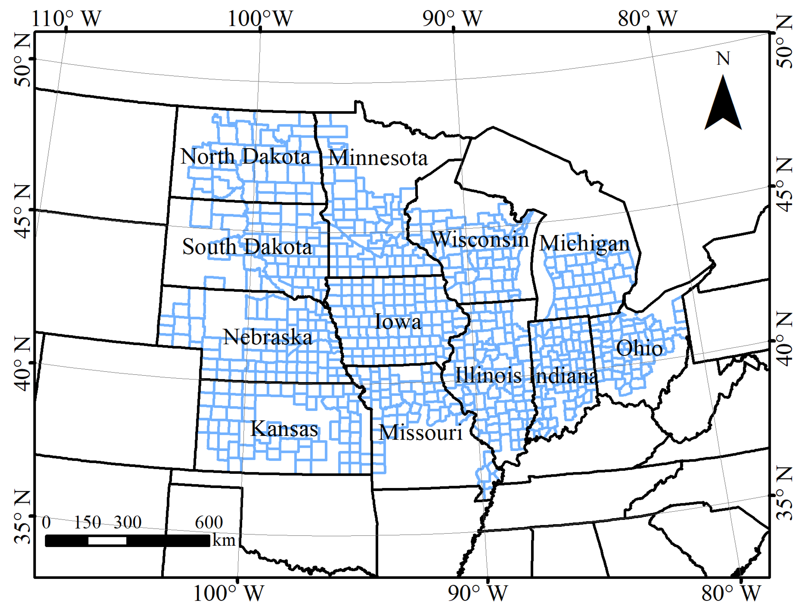
2.1. Study Region

The focal area for the study was the Corn Belt of the USA. A total of 766 agricultural counties selected for the study were located in 12 states, namely Minnesota, South and North Dakota, Wisconsin, Michigan, Nebraska, Iowa, Illinois, Indiana, Ohio, Kansas and Missouri, which accounted for 89% of US corn production in 2016 [19]. The distribution of these counties is shown in Figure 1.

2.2. Datasets

2.2.1. Crop Yield and Area

County-level corn yields were obtained from the National Agricultural Statistics Service (NASS) of the US Department of Agriculture (USDA) (https://quickstats.nass.usda.gov/ (accessed on 21 April 2019)). The yield unit was converted from bushels acre⁻¹ to kg ha⁻¹. As some counties had no individual annual yield data, the total number of yield samples was n = 6783 (i.e., S number of years with data per county from 2008–2018), which was less than the theoretically possible n = 8514. Crop planting coverage was obtained from the Cropland Data Layer (CDL, http://nassgeodata.gmu.edu/CropScape/ (accessed on 21 April 2019)) with a 30 m resolution. CDLs needed to be reprojected to match the geographic projection of moderate resolution imaging spectroradiometer (MODIS, Collection 6) data, which were used to distinguish pixels dominated by corn from those dominated by other land cover types.

2.2.2. Satellite Data

Ordered from the National Aeronautics and Space Administration (NASA) (https://ladsweb.modaps.eosdis.nasa.gov/ (accessed on 12 October 2019)), three MODIS-based datasets (i.e., EVI, LST and LAI) included four tiles for the USA from 2008–2018 (MODIS tile numbers h10v04, h11v04, h10v05 and h11v05), which were reprojected to the universal transverse mercator (UTM) using the MODIS reprojection tool (MRT).

EVI [36], LST (daytime) and LAI were a composite dataset of 16, 8 and 8 days, with a spatial resolution of 1000 (i.e., MYD13A2 product), 1000 (i.e., MYD11A2 product) and 500 (i.e., MYD15A2H product) m, respectively. All data were collected by the Aqua satellite which collected data at the time of maximum atmospheric evaporative demand (approximate satellite overpass: 14h30). This condition ensured that EVI, LST and LAI data were obtained for the time of day when ET was the greatest.

In the 16- or 8-day time-series images for EVI, LST and LAI, monthly images were obtained by averaging four EVI, two LST or two EVI composite images [38,39]. For monthly time-series images, EVI, LST and LAI values were extracted from corn pixels identified using CDL data and then averaged to obtain mean values for each county [40].

2.3. Methods

An advanced method of LR and three representative ML methods were tested to analyze and describe the relationships between yield and three selected satellite-derived indices (i.e., EVI, LAI and LST). The selected methods were as follows: LASSO, SVR, RF and LSTM.

2.3.1. LASSO

As a regularized linear regression method using shrinkage and selection, LASSO was selected as a benchmark model relative to the three ML algorithms. In addition, it minimized the absolute value sum of coefficients by imposing a constraint on model parameters causing regression coefficients for some variables to shrink toward zero, ultimately resulting in a parsimonious model [41]. Moreover, LASSO performed automated feature selection and introduced L1 regularization to avoid overfitting during the construction of the yield estimation model. Due to the autocorrelation of input indices (i.e., EVI, LST and LAI), the LASSO method was used to automatically remove redundant information.

2.3.2. SVR

SVR is a regression algorithm used to find an optimal regression plane where sample points are closest to it. The key to the SVR algorithm is the choice of the kernel function, which can be either linear or nonlinear according to the relationship between target sample values, and input features. A linear model was subsequently built in feature space for balancing the minimization of errors and overfitting. The optimized kernel function was adopted to determine whether the relationships between the three satellite-derived indices and yield were linear or nonlinear.

Four kernel functions (liner, polynomial, radial basis and sigmoid) were modeled, and the kernel function with the best model performance was selected as the modeling kernel function. It was necessary to “tune” the overfitting penalty (value range and step size, 1–10 and 1) and gamma (0–1, 0.02), independent term (−3–3, 0.2) and polynomial degree (1–7, 1) for these kernel functions.

2.3.3. RF

RF is a supervised ensemble algorithm where every input feature is trained using its respective target value, whose performance mainly depends on the establishment of numerous decision trees based on input features, and target values selected randomly and integrated for regression. The number of trees in the “forest” (value range and step size, 10–500 and 50), the maximum depth of trees (10–100, 5) and the maximum number of features (1–number of variables, 1) to consider in the case of looking for the best split were three user-defined hyper-parameters needing to be tuned. With low sensitivity to outliers and high computational efficiency, RF is not prone to overfitting [42], which is insensitive to multi-collinearity and can be used to efficiently analyze high-dimensional datasets for significant variables. These properties made it a suitable analytical tool for use in the three satellite-derived indices (i.e., EVI, LST and LAI) for the six-month GS.

2.3.4. LSTM

As a recurrent neural network (RNN) where a sequence of inputs are processed at nodes with directed connections, LSTM networks can be used to identify important features related to time-series because of maintaining a chain structure incorporating time steps in crop yield modelling [17,43]. Each step takes information from the previous one and outside input (from feature space–new EVI, LST and LAI values), and provides output for the next one. In addition, the algorithm can retain the key information of input signals during the training process and ignore less important aspects. The LSTM model for corn yield estimation was implemented using TensorFlow, an open-source ML library in Python.

We first defined three bi-directional LSTM layers to learn time-continuous and satellite-based input features, and a fully connected layer with one neuron, which was used to output a yield prediction value (pre1). Then, the geographic location, named county ID, was considered to have effects on crop growth, which was learned by two fully connected layers with one output layer of one neuron activated by the sigmoid function, obtaining a range of values (0, 1) (pre2). Lastly, pre1 was regulated by pre2 to derive the final yield (pre2 × pre1).

Specific parameter settings were as follows:

(1) Neurons: Tuning the number of neurons on each LSTM layer and one fully connected layer;

(2) Regularization: L2;

(3) Loss function: Huber;

(4) Optimizer: Adam;

(5) Epoch: The number of epochs was set at 1000. The training applied the EarlyStopping callback function from Keras API [17], with a patience parameter (the number of epochs without improvement after which training was stopped) equivalent to 100 to avoid overfitting;

(6) Data dividing: We assumed that the prediction year’s yield was strongly correlated with the yield of the previous year, but with a progressively weaker correlation for each preceding year, for a period of three years. The proportion of training samples in each year was different, with most training samples obtained from the year preceding the prediction year. For example, the proportions of training samples for the years 2008–2016 were 1:2:4:6:8:10:12:14:16, with 2018 as the prediction year and 2017 as the validation year.

2.4. Experiment Design

Data were preliminarily explored by determining the spatiotemporal pattern of correlations between different satellite-derived indices and corn yield and selecting significant months for yield estimation. The relationship metric used was the Pearson correlation coefficient (r).

(1) Temporal correlation analysis: The monthly county-level correlations between yield and different indices in all years were calculated to investigate whether corn yield was similarly or uniquely sensitive to satellite-derived indices in different months.

(2) Spatial pattern of correlation analysis: To further investigate whether spatial differences existed in yield–satellite index relationships, the month with the highest correlation was selected according to the absolute value, and the spatial pattern of this correlation for all counties was examined in that month.

Three groups of experiments were designed using seven inputs and four empirical methods to address the research questions mentioned in this paper. Seven inputs were four combinations of indices, namely EVI + LST + LAI, EVI + LST, EVI + LAI, and LST + LAI, and three individual indices, namely EVI, LST and LAI, while four empirical methods included one method of LR (LASSO) and three nonlinear methods of ML, namely SVR, RF and LSTM.

(1)

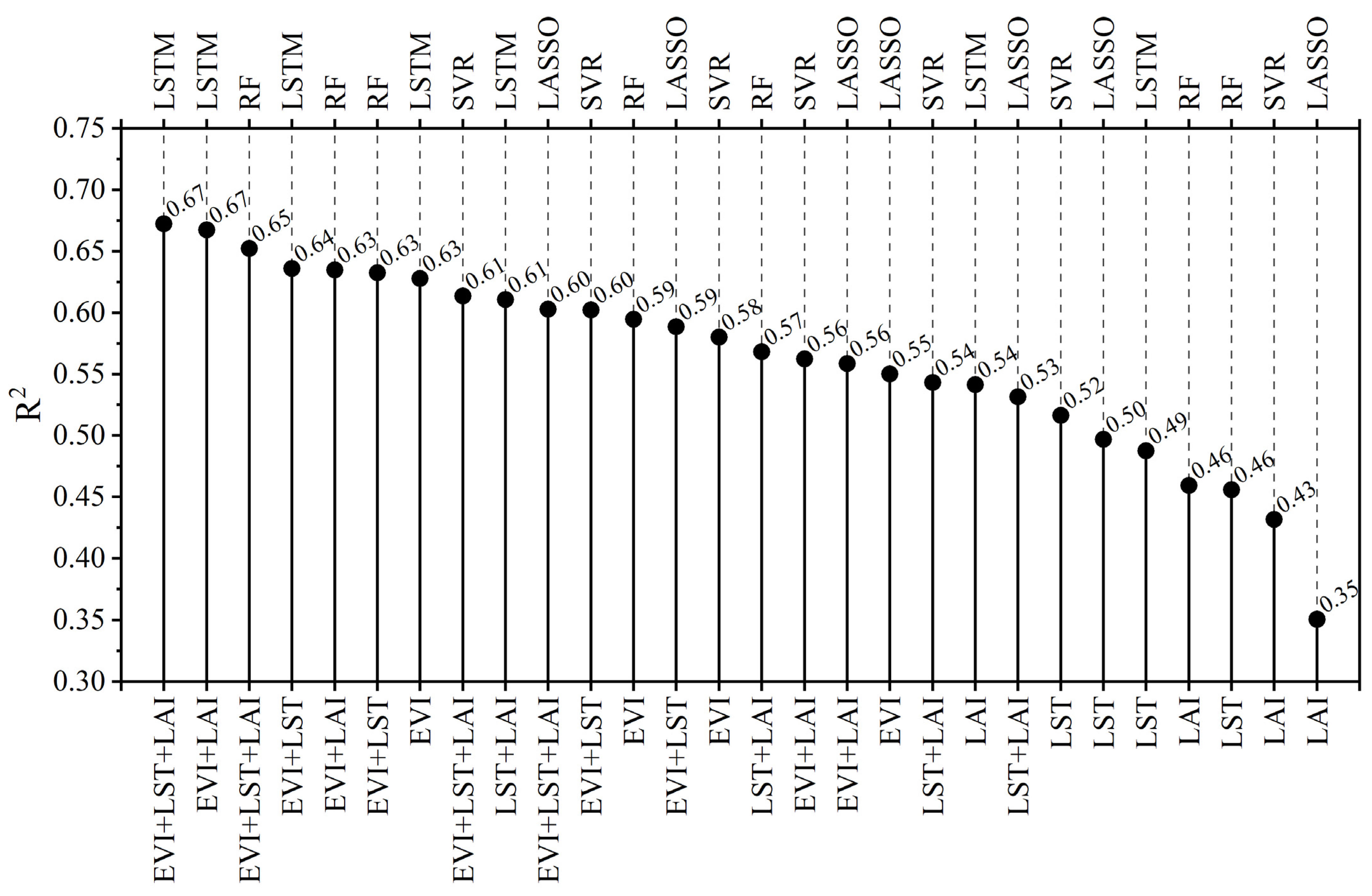
The first research question was answered by the first group of experiments. That is, was the performance of the yield prediction model affected by the number of indices used as input variables?

(2)

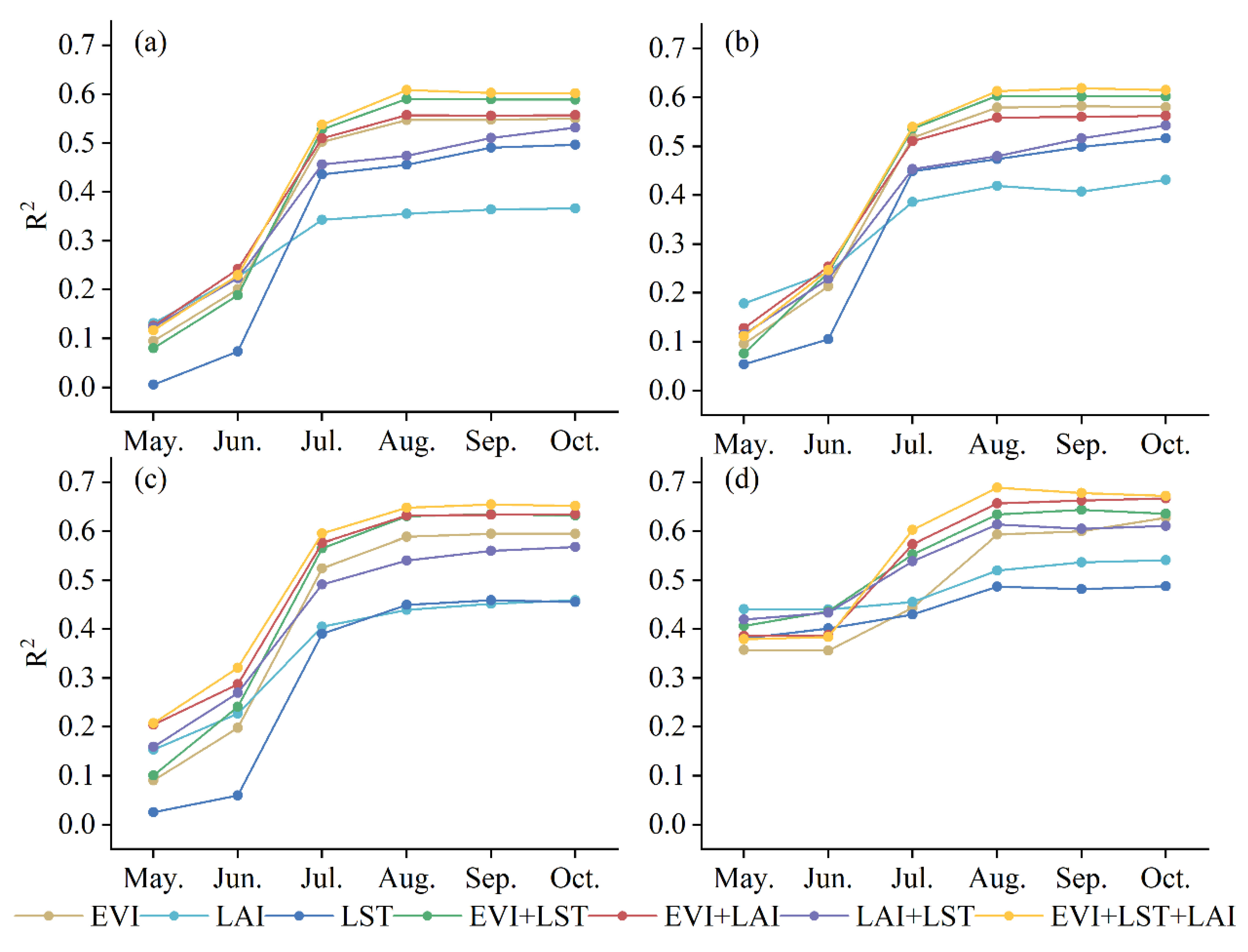
The second question was answered by designing the second group of experiments that focused on the temporal progression of model performance for successive months and was used to highlight predictive performance changes within the season of the model for corn yield. For any month during the GS, satellite data from the beginning of the GS to the current month were used as inputs to predict the corn yield at harvest. The approach allowed for the determination of the progression in model performance for different satellite data inputs. These results helped identify the added value of satellite data over time for the prediction within the season. In addition, the optimal time during the GS could be identified for predicting corn yield using different methods and inputs. For example, the earliest month for obtaining an accurate corn yield estimate could be identified at the county level.

(3)

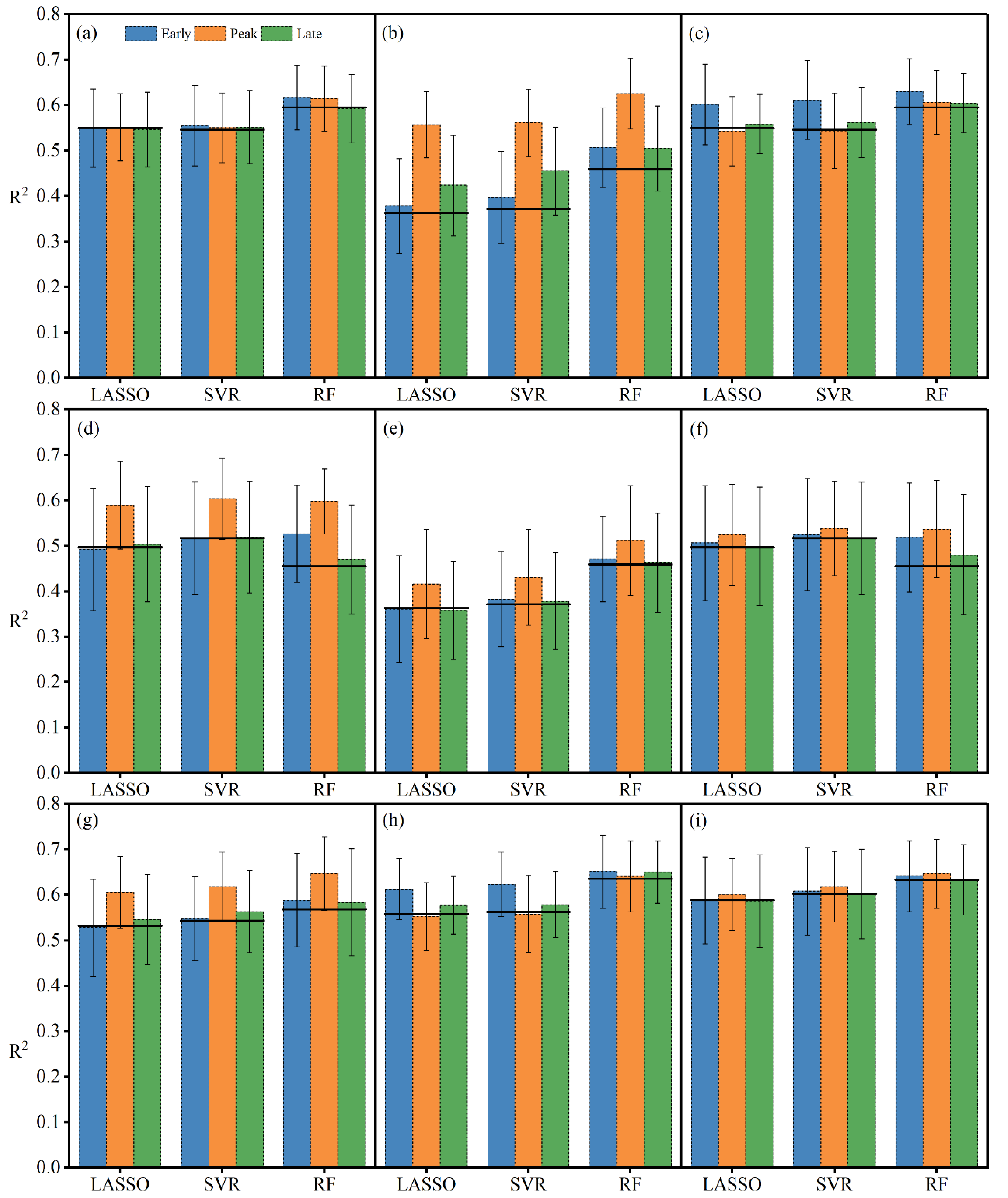
The third group of experiments was designed to investigate how satellite data contributed to yield prediction in different growing stages (the third question). Three growing stages were defined for use in this study:

(a)

The early growing stage (GS_early) (Planting–Jointing, May–June);

(b)

The peak growing stage (GS_peak) (Jointing–Dough, July–August);

(c)

The late growing stage (GS_late) (Dough–Harvest, September–October).

To assess the influence of three satellite-derived indices in different growth stages on crop yield estimation, one or two satellite-derived index datasets from the whole GS, but only one satellite-derived index dataset during one specific growing stage about the following three options, were used.

Option 1: Only one satellite-derived index dataset was used during the GS_early (“one satellite in the early stage + one or two satellites in the whole season”);

Option 2: Only one satellite-derived index was used during the GS_peak (“one satellite in the peak stage + one or two satellites in the whole season”);

Option 3: Only one satellite-derived index was used during the GS_late (“one satellite in the late stage + one or two satellites in the whole season”).

We only applied the three methods (LASSO, SVR and RF) to the satellite-derived indices, and then compared the predicted R² of the above three options model results with the benchmark model results. The benchmark model results were obtained with one or two satellite-derived indices of the whole GS. The experiment determined the stage where one satellite-derived index had more additional value for final yield prediction.

2.5. Model Training and Evaluation

The three variables were normalized to have a mean of zero and unit standard deviation (SD) before model training, making it possible to compare the three satellite-derived index variables in models. The performance of crop yield models is dependent on their predictive power for real-world yield in a future year. Thus, the yield prediction performance of each model was evaluated by an out-of-sample test, to be specific, a “leave-one-year-out” cross-validation (LOYO-CV) test [31]. With 11 years of data (2008–2018) available, 10 years were used to train models, with one year removed to be used later as an independent dataset for testing purposes. We determined the best hyper-parameters for the LASSO, SVR and RF methods from empirical candidates, based on the cross-validated R² values calculated by applying three-fold cross-validation using only training data. The whole process was repeated 11 times, namely once for each of the 11 years of data. The LSTM method was also trained by taking the LOYO-CV approach.

We applied the optimized models to the testing dataset and calculated the predicted R², which was then used to compare the performance of different models for yield estimation for the first experiments. In the second and third groups of experiments, the mean predicted R² values were used for comparing the performances of different models and testing the contributions of different data inputs.

3. Results

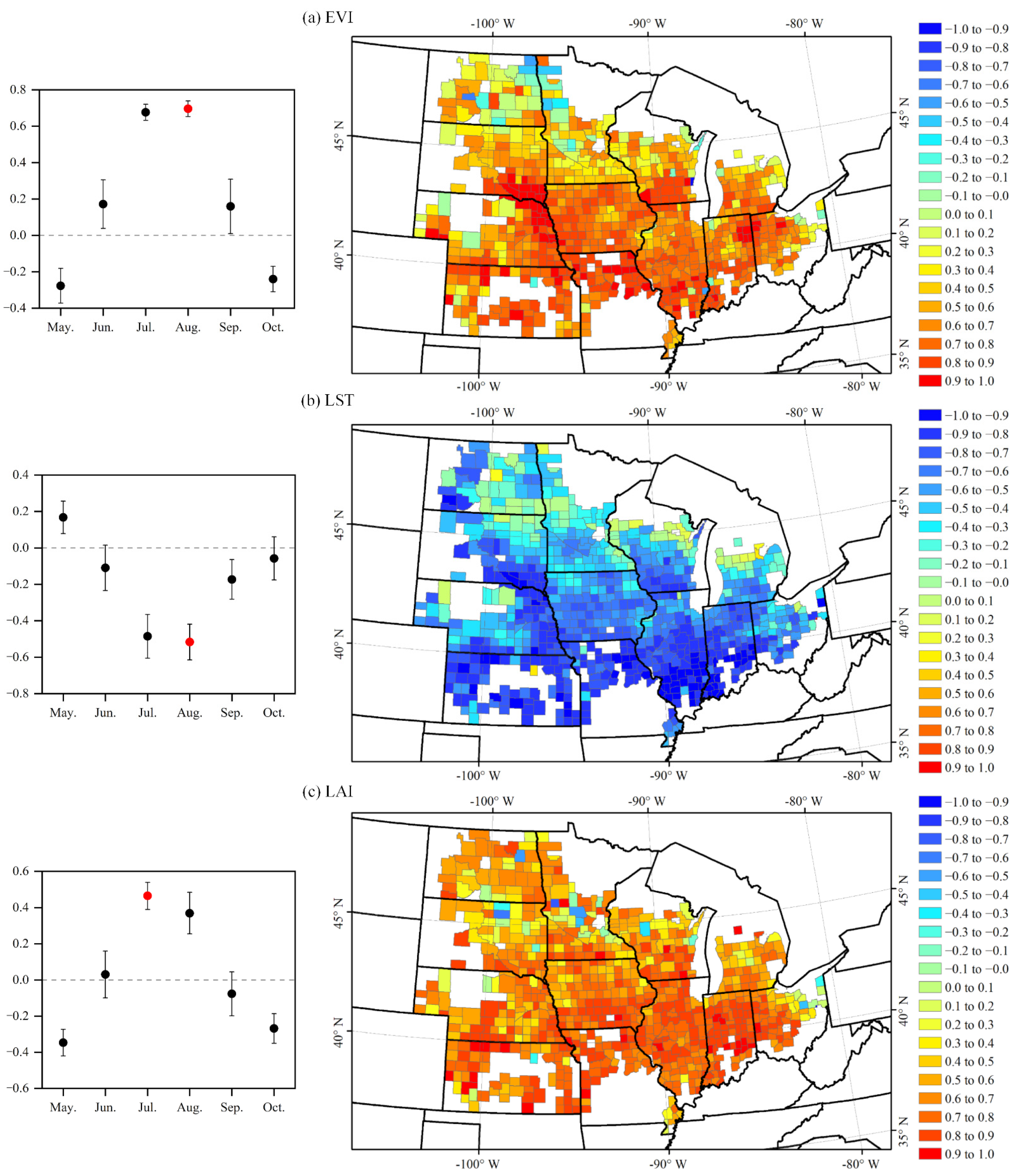
3.1. Spatiotemporal Correlations between Different Variables and Corn Yield

The spatiotemporal patterns of correlations between corn yield and satellite-derived index variables are shown in Figure 2. Linear correlations between corn yield and input variables provided important clues regarding the importance of predictors. The correlation for the temporal evolution of sequential variables is presented in Figure 2 (left panels). The three sources of satellite data displayed similar patterns of variation. The correlation between EVI or LAI and corn yield first increased steadily until the peak around July or August, and then decreased. The rise and fall in LST had an adverse trend in the relationship between EVI or LAI and yield. In general, EVI and LAI variables related to crop growth both had the highest positive correlation with yield in July or August, but then the highest negative correlation in May and October, which might indicate that yield was most sensitive to the intensity of growth, the growth of seedlings and the degree of attenuation in the GS_peak (July–August), GS_early (May) and GS_late (October), respectively. Generally, the thermal environment related to LST had the highest negative correlation with yield in August and the highest positive correlation in May, indicating that yield was most sensitive to high temperature in the GS_peak and low temperature in the GS_early. In addition, the maximum correlation with the highest absolute value occurred around the GS_peak (i.e., July or August) for each variable.

The spatial patterns of correlations between corn yield and different variables (right panels in Figure 2) during the GS_peak were homogenously high for all the three satellite-derived indices (

Table 1. R values for the correlations of each two indices for all counties. The correlations were the r values between each satellite-derived index during the peak GS and corn yield in each county (right panels in Figure 2).

	EVI	LST	LAI
EVI	-	−0.56 *	0.38 *
LST	-	-	−0.49 *
LAI	-	-	-

* Significant at p < 0.01.

), with the exception that small counties in the north and west were less well correlated with yield. The spatial correlation for LST was the opposite of that for EVI and LAI (Table 1). The negative correlation between LST and EVI (LAI) across a variety of spatial and temporal scales was previously reported by Gao et al. [44]. Overall, the spatiotemporal patterns of relative similarity for the whole Corn Belt indicated that one model could be constructed for the whole region rather than different models for different sub-regions within the Corn Belt at the county level.

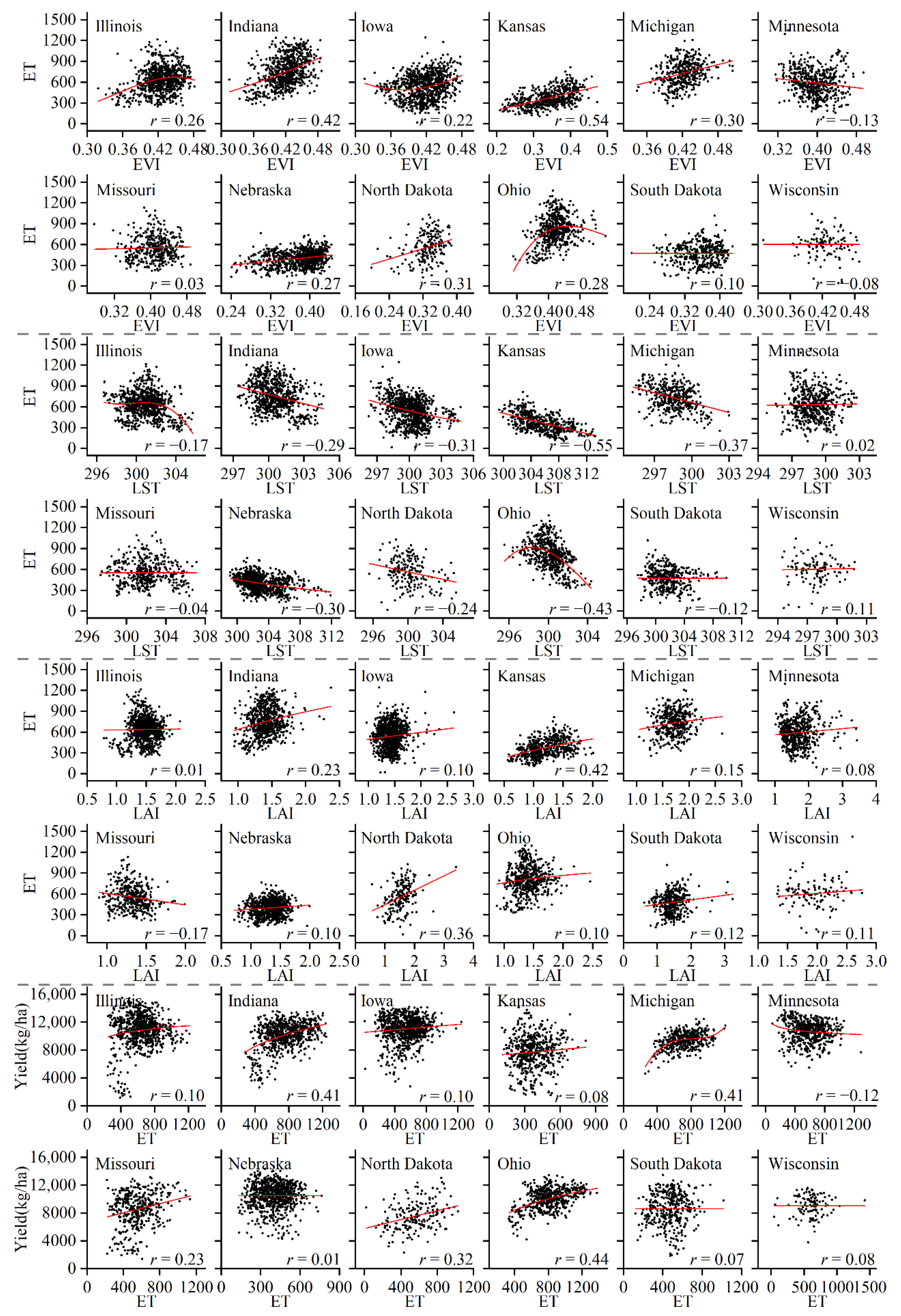
3.2. The Relationships between the Three Indices and ET and the Relationship between ET and Corn Yield

There is a positive correlation between ET and EVI (Figure 3). Among the twelve states, six states had a positive linear correlation, four states had a positive nonlinear correlation, and two states had a negative linear correlation. Among the ten states with a positive correlation, four states had a significant relationship (r > 0.30), and six states had an insignificant relationship. This relationship reflects that the more corn canopy coverage there is, the stronger the photosynthesis will be, the more water that needs to be absorbed and transported, and the more water that will be lost.

There is a negative correlation between ET and LST (Figure 3). Among the twelve states, six states had a negative linear correlation, four states had a negative nonlinear correlation, and two states had a positive linear correlation. Among the ten states with a negative correlation, five states had a significant relationship (r > 0.30), and five states had an insignificant relationship. Increased temperature leads to increased transpiration, making the stomata close to prevent water loss of corn leaf cells.

There is a positive correlation between ET and LAI (Figure 3). Among the twelve states, seven states had a positive linear correlation, four states had a positive nonlinear correlation, and one state had a negative linear correlation. Among the eleven states with a positive correlation, two states had a significant relationship (r > 0.30), and nine states had an insignificant relationship. The larger LAI, the more exposure of leaves to light, and the more water is transpired into the atmosphere through stomata.

Corn yield correlates positively with ET (Figure 3). Among the twelve states, seven states had a positive linear correlation, four states had a positive nonlinear correlation, and one state had a negative nonlinear correlation. Among the eleven states with a positive correlation, four states had a significant relationship (r > 0.30), and seven states had an insignificant relationship. The more ET, the more water is consumed by corn growth, and the higher the productivity and yield.

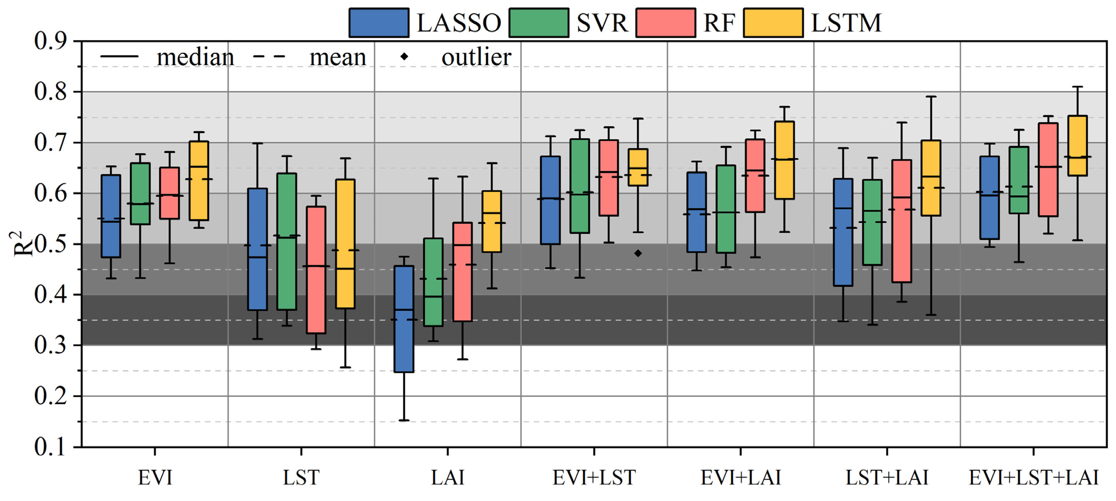
3.3. Multi-Model Performance in Corn Yield Estimation

Figure 4 shows the results of performance in the first group of experiments when the four methods were applied to different inputs with all month data. The ranking of these inputs from high to low was as follows: EVI + LST + LAI (mean x and SD of all predicted R² values for the four methods, 0.64 and 0.08) > EVI + LST (x, 0.61; SD, 0.08) > EVI + LAI (x, 0.61; SD, 0.09) > EVI (x, 0.59; SD, 0.08) > LST + LAI (x, 0.56; SD, 0.11) > LST (x, 0.49; SD, 0.13) > LAI (x, 0.45; SD, 0.12). As expected, the EVI + LST + LAI input performed best, followed by the paired indices and the single-index variable. However, the single-index EVI input exhibited better performance than the paired LST + LAI input, suggesting that EVI was better for corn yield estimation than the combination of LST and LAI. For the model performance with paired inputs, the EVI + LST combination performed best, better than either the EVI + LAI or LST + LAI combination. For single-index inputs, EVI data performed better than LST and LAI ones. The results in Figure 4 answered the first research question, namely whether the combination of all three satellite-derived data inputs showed the best performance in estimating corn yield, followed by paired satellite data combinations.

The ranking of the four methods from high to low was as follows: LSTM (mean x and SD of all predicted R² for all different inputs, 0.61 and 0.11) > RF (x, 0.57; SD, 0.12) > SVR (x, 0.55; SD, 0.11) > LASSO (x, 0.53; SD, 0.12). Overall, the LSTM NN analysis produced the highest R² values, followed by RF and SVR, with LASSO producing slightly inferior performance. These results were consistent with those reported in other studies [33], noting that nonlinear methods (i.e., LSTM, RF and SVR) outperformed the method of LR (i.e., LASSO). This could be attributed to the nonlinear nature of most correlations between yield and different indices.

The ranking of model performance for the four methods and different inputs has been shown in Figure 5. The three-fold EVI + LST + LAI combination and LSTM method produced the highest R² value (mean for the results derived from LOYO-CV) of 0.67, followed by EVI + LAI and LSTM with an R² value of 0.67 and EVI + LST + LAI and RF with an R² value of 0.65. For the single-index inputs, EVI and LSTM achieved the best results with an R² value of 0.63, which was higher than most models. LSTM produced the best predictive performance of the four methods, when applied to all different inputs, except for LST. When applying LASSO and SVR, choosing EVI + LST + LAI allows for optimal yield estimation.

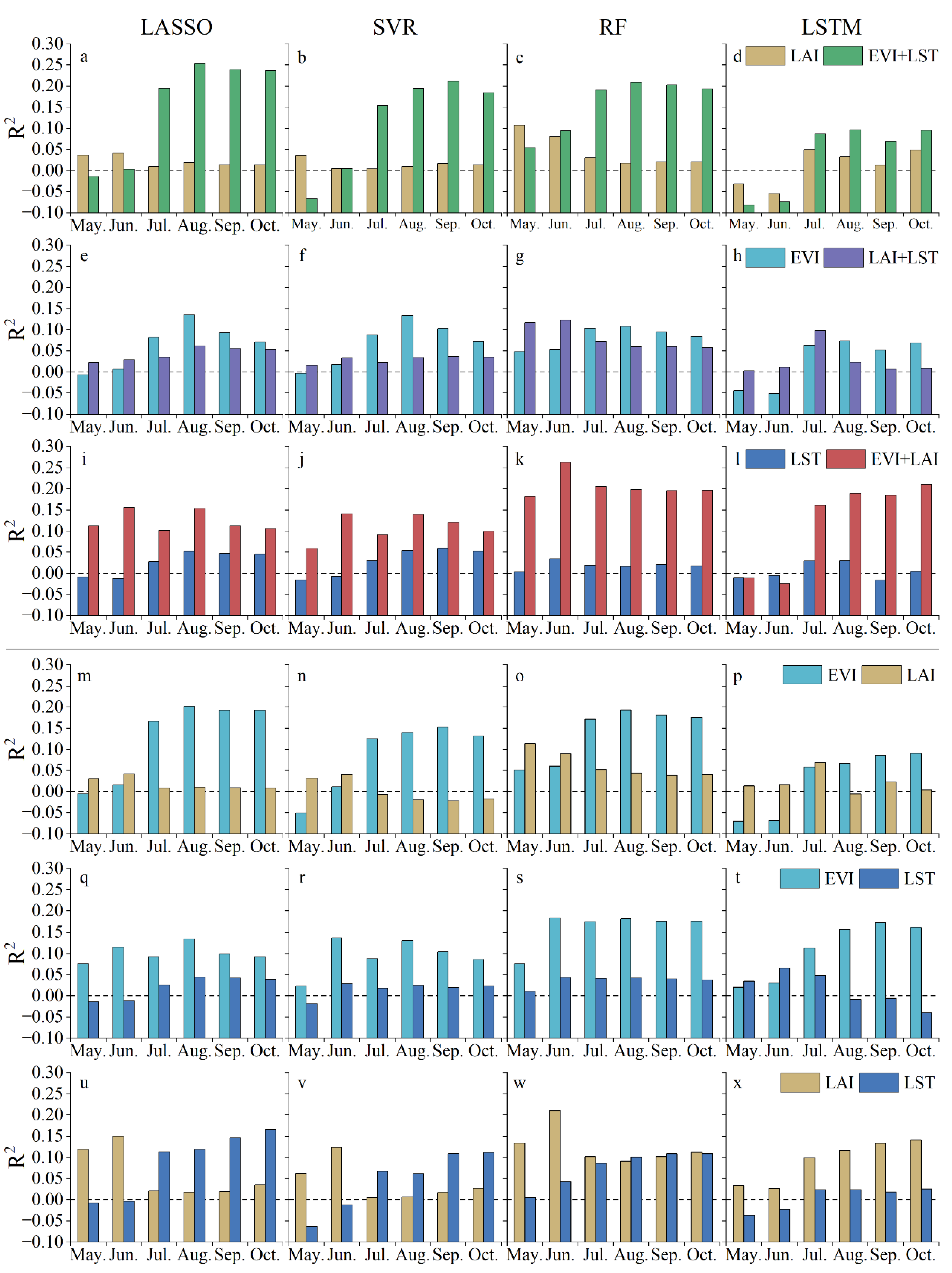
3.4. Quantification of Unique and Shared Information from Different Satellite Data

Figure 6 shows the contribution of sequential information on satellite-derived indices (EVI, LST and LAI) to the prediction of corn yield during different growth stages (GS_early, GS_peak and GS_late).

First, the conditions of one index dataset for all months (i.e., the whole GS) and one index dataset for only one specific growth stage were described.

(1) The models constructed using EVI for all months and LAI for a specific growth stage showed an increased R² value ranging from 0.00 to 0.02 (Figure 6a). All the R² values for each method in the three stages improved slightly or even declined (bars above or below the solid line in Figure 6a) after the combination of a specific LAI and all EVI, meaning that LAI throughout the whole GS could not provide unique and added information for better yield estimation when combined with EVI. In contrast, the increased R² values (0.01–0.19) for all LAIs and a specific EVI (Figure 6b) were higher than those in Figure 6a. Notably, the largest improvement of R² (0.17–0.19) was found in the models with the peak EVI, while smaller changes were evident for those in the other two stages, especially the early EVI. EVI played different roles as the peak EVI reflected most crop growth states when the crop was exposed to both biotic and abiotic stresses. The crop in the GS_early was in the vegetative stage, indicating that EVI was not a good indicator of biomass and final yield.

(2) The models constructed using all EVI and a specific LST showed an increased R² value ranging from −0.01 to 0.07 (Figure 6c). The largest improvement of R² (0.04–0.07) was found in the models with the early LST, while smaller changes were apparent for those in the other two stages. By comparison, the increased R² values (−0.01–0.14) for all LST and a specific EVI (Figure 6d) were higher than those in Figure 6c, while the largest improvement of R² (0.09–0.14) occurred in the GS_peak, especially for RF models.

(3) The models constructed using all LAI with a specific LST showed an increased R² value ranging from −0.01 to 0.06 (Figure 6e). The largest improvement of R² (0.05–0.06) was found in the models with the peak LST, while smaller changes were apparent for those in the other two stages. In contrast, all LST and a specific LAI demonstrated an increased R² value (0.00–0.08, Figure 6f), while the largest improvement of R² (0.02–0.08) occurred in the GS_peak.

Then, the conditions for paired indices for all the months with one index for only one specific growth stage were described. The models constructed using LAI + LST and a specific EVI showed an increased R² value ranging from 0.00 to 0.08 (Figure 6g). The largest improvement of R² (0.07–0.08) was found in the models with the peak EVI, while smaller changes were apparent for those in the other two growth stages, especially the early stage EVI. In contrast, the models constructed using the EVI + LAI combination and a specific LST showed an increased R² value ranging from −0.01 to 0.06 (Figure 6h). LST had a greater increase in R² (0.02–0.06) during the GS_early than during the other two growth stages, although the contribution of the LST during the GS_peak slightly reduced the performance of the EVI + LAI combination derived using LASSO and SVR methods. The increased R² values produced using the RF method in the GS_early and GS_late were smaller than those obtained using LASSO and SVR methods. Finally, the increased R² values (0.00–0.02) for all stages using the EVI + LST pairing and a specific LAI (Figure 6i) were smaller than those in Figure 6g,h.

In addition, Figure 7 summarizes the temporal variation of the R² values for the four methods in more detail using different combinations of satellite-derived input variables. All the R² trajectory curves derived from the four methods showed a similar pattern.

(1) For any satellite-derived inputs, R² values increased with time as more input data became available. Model performance usually reached saturation during the GS_peak (i.e., August).

(2) The characteristics of different inputs after July were as follows: The three-fold index input (EVI + LST + LAI) was superior to paired index inputs, followed by individual index variable inputs. Overall, the EVI + LST pairing performed better than EVI + LAI and LAI + LST pairings. For single inputs, EVI only performed better than LAI and LST. Interestingly, EVI alone performed better than the LAI + LST pairing.

Additionally, obvious differences were found in the performance of LAI as a single input and other input variables (i.e., EVI and LST as single inputs, paired inputs and three-fold inputs) for the three methods (LASSO, SVR and RF), and also LST as a single input and other input variables (i.e., EVI and LAI as single inputs, paired inputs and three-fold inputs) for the LSTM method.

For the whole GS, LAI as a single input started with much higher performance (~0.1–0.2), and achieved a much lower increase in performance later (an increase of ~0.2–0.3) compared with EVI and LST for the three methods (LASSO, SVR and RF), with most of the increased performance achieved before July. In contrast, both EVI and LST as single inputs started with relatively poor performance (~0.0–0.1) but produced much greater increases (an increase of ~0.4–0.5) later in the GS. These later increases exceeded those produced for LAI in the same stage. The numbers in brackets represent the predicted R² values. These results indicated that LAI during the GS_early provided more information than EVI or LST. In contrast, both EVI and LST in the GS_peak and GS_late offered more information for corn yield estimation. All the inputs for the LSTM method started with much higher performance than those for the other three methods (LASSO, SVR and RF), which was related to the LSTM framework. It indicated that the LSTM method performed better in May and June, and failed to detect time-series features from May to June.

Furthermore, the focus was on the value added by each satellite-derived data input as the season advanced (from May to October) for different data combinations (Figure 8). The results for the three-fold combination (EVI + LST + LAI) are shown in a series of sub-figures (Figure 8a–l) in Figure 8.

(1) The contributions of LAI declined as corn grew from the GS_early to the GS_peak and then stagnated from the GS_peak to the GS_late, while those of the EVI + LST pairing initially increased and then stagnated using the three methods (LASSO, SVR and RF). For the LSTM method, the contributions to yield made by both LAI as a single input and the EVI + LST paired input first rose and then decreased over the duration of the GS.

(2) Over the GS, the contributions of EVI to the prediction of yield increased before decreasing based on different trends exhibited by the LAI + LST pairing for the three methods (LASSO, SVR and RF). For the LSTM method, the contributions of EVI to yield prediction increased from the GS_peak to the GS_late, whereas those of the LAI + LST pairing decreased.

(3) The contributions of LST to yield prediction increased from the GS_early to the GS_late, whereas those of the EVI + LAI pairing for each of the three methods (LASSO, SVR and RF) declined. For the LSTM method, the contributions of LST as a single input and the EVI + LAI pairing both declined from the GS_peak to the GS_late.

(4) For the LSTM method in particular, the value added by a single or a paired input was negative in the GS_early. This disparity could be mostly attributed to different model frameworks. The LSTM method considered the temporal variability of input data from the early GS to prediction time, but the time-series data from May to June could not provide a sufficient number of distinctive time-series features for training purposes.

Figure 8m–x shows the added value in paired inputs (i.e., EVI + LST, EVI + LAI and LAI + LST).

(1) The EVI + LAI pairing produced similar patterns for the three methods (LASSO, SVR and RF) over the duration of the GS. The value added by EVI increased from the GS_early to the GS_peak and then stagnated, while that added by LAI almost showed an exactly reversed pattern. For LSTM, the value added by EVI increased from the GS_early to the GS_peak and then stagnated, while that added by LAI increased and then decreased.

(2) For the EVI + LST pairing, EVI had increased (GS_early–GS_peak) and then decreased (GS_peak–GS_late) added value with LASSO and SVR. However, EVI had increased (GS_early–GS_peak) and then stagnated (GS_peak–GS_late) added value with RF, and increased added value with LSTM. The value added by LST initially increased (GS_early–GS_peak) and then stagnated (GS_peak–GS_late) for LASSO, SVR and RF, but increased (GS_early–GS_peak) and then decreased (GS_peak–GS_late) for LSTM.

(3) For the LAI + LST pairing, the value added by LST initially increased (GS_early–GS_peak) and then stagnated (GS_peak–GS_late), while that added by LAI decreased initially (GS_early–GS_peak) and then stagnated (GS_peak–GS_late) with the three methods (LASSO, SVR, and RF), but increased from the GS_early to the GS_late for LSTM.

4. Discussion

4.1. Yield Prediction Based on Satellite Data and ML

Each index contributed to corn yield estimation, whether it is a specific growth stage (Figure 6) or the whole GS (Figure 8). Previous studies have focused on estimating yields using two indices [19,20]. In this study, compared with using paired indices or indices used as single inputs, the three-fold combination of EVI + LST + LAI produced the best results for corn yield prediction, using any of the four methods in the study. At the same time, adding data with time during the whole GS improved the performance of corn yield prediction models. Based on the overall situation of all inputs, it was found that nonlinear methods (i.e., SVR, RF and LSTM) were superior to the linear method (i.e., LASSO) [33], among which the best performing one was LSTM [17,41].

The three indices as single inputs had the highest correlation with corn yield around the GS_peak (July or August) (Figure 2), which largely explained why individual index-based models reached their best performance around the GS_peak (Figure 6). Compared with the EVI model showing the best performance for a single input, LST added as a predictor (EVI + LST) after June improved the performance of national yield prediction, and LAI added upon the EVI + LST pairing further improved prediction performance from July to October.

4.2. Unique and Shared Contributions of Satellite Data to Yield Prediction

The three satellite-derived indices have always been the main satellite data for the monitoring of crop growth and the prediction of yield. Based on identifying the contributions of satellite data relative to meteorological data to crop yield estimation [3,33], this study complements the shared and unique contributions of the three satellite indices, which can support predicting and estimating crop yield more scientifically and accurately.

Firstly, about 56%, 40% and 49% of corn yield variability could be explained by only using EVI, LAI and LST, respectively. However, the better results for crop prediction could be obtained by using two paired indices as inputs, namely EVI + LAI, or the three-fold combination, namely EVI + LST + LAI. The best results were obtained by use of the three-fold combination.

Secondly, the increased R² from a single index in a specific period (the GS_early, GS_peak and GS_late) combined with either one or two index datasets in the whole GS were analyzed.

(1) The paired combination: The increased R² values from a specific LAI combined with the EVI of the whole GS were much smaller than those from a specific EVI combined with the LAI of the whole GS. The increased R² values from a specific LST combined with the EVI of the whole GS were much smaller than those from a specific EVI combined with the LST of the whole GS. The increased R² values from a specific LST combined with the LAI of the whole GS were similar to those from a specific LAI combined with the LST of the whole GS. The finding substantiates that EVI supplies more information than LAI and LST for corn yield estimation [19,20], and LAI and LST supply similar information.

(2) The three-fold combination: The increased R² values from a specific EVI combined with the LAI + LST of the whole GS were bigger than those from a specific LST combined with the EVI + LAI of the whole GS, followed by a specific LAI combined with the EVI + LST of the whole GS. The finding further substantiates that EVI supplies more information than LST (LAI) for accurate corn yield estimation.

Thirdly, the focus was on the specific periods (the GS_early, GS_peak and GS_late) and indices (EVI, LST, LAI) showing more unique contributions.

(a) Analysis of the paired combination: For the EVI + LAI pairing, GS_peak EVI was found to provide more corn yield information in the GS_peak than in the other two stages, suggesting that GS_peak EVI contained biotic or abiotic stress-related information [3,33], which might not have been captured by accumulated LAI [20]. No differences between stages were apparent for LAI data, suggesting that no unique individual information existed across the whole season for LAI. For the EVI + LST pairing, LST provided more information in the GS_early than in the other two stages, suggesting that GS_early LST was critical for the growth of crops and included more temperature information of bare land. For the LAI + LST pairing, we found that the GS_peak LST (GS_peak LAI) provided more information than the other two stages.

(b) Analysis of the combination of the three-fold variable: The GS_peak EVI (GS_early LST) provided more corn yield information than the other two stages. However, no such differences were apparent for LAI, suggesting that no unique individual LAI information existed in any special stage across the whole season (Figure 6).

4.3. Satellite Variables and Evapotranspiration

According to the unique information of satellite-derived variables on corn yield, the explanation of EVI, LST and LAI on corn yield from an evapotranspiration perspective was discussed based on the combination input of the three variables, which was consistent with the actual factors affecting the ET of corn [45,46,47]. In the early and middle vegetative stages, the corn canopy coverage density was relatively small. As a result, ET was dominated by evaporation from the soil surface and not via the plant. Soil evaporation in the early and middle vegetative stages was mainly determined by soil surface temperature (LST used as a surrogate value) [48]. At full crop canopy, namely in the late vegetative stage and early reproductive growth stage, when corn grows vigorously and needs a lot of water, the crop canopy closes to completely shade the soil surface. During these stages, most ET could be attributed to transpiration. Corn transpiration in these stages was related to the corn canopy coverage (EVI) [49], without the canopy temperature (indirectly measured using LST) and number of stomata (LAI). Corn stomata (LAI) during the whole GS had no significant implications for ET and yield.

4.4. The Constructed LSTM Framework

The main methods for yield prediction and estimation, namely LASSO, SVR and RF, usually produce acceptable results, but they were not developed according to time-ordered data analysis. Since EVI, LST, and LAI were inherently temporal in nature, with the future yield predictions dependent on the past state of these variables, we could assume that algorithms that could be trained to identify temporal patterns would outperform those that did not account for this variation. This assumption was confirmed by the results of our study. LSTM NN outperformed LASSO, SVR and RF, which was consistent with the results presented in other studies [33,35]. Interestingly, LSTM was better at predicting crop yields, based on data collected for May and June, than the other three methods. This finding indicated that LSTM method was best suited for making yield predictions based on data collected in the GS_early.

4.5. Limitations and Outlook

(1) The use of additional variables perhaps improves the accuracy of the yield prediction model. For example, solar radiation has been known to influence actual evapotranspiration [23]. We did not include solar radiation data in this study as the spatial resolution of the solar radiation data was too coarse. The solar radiation data used in the research [23] from the Monthly Ed4A of CERES_SYN1deg product had a spatial resolution of 8 km (http://ceres.larc.nasa.gov/ (accessed on 17 January 2020)). We tried to add this radiation data to the combined EVI, LST and LAI model, but the accuracy of the corn yield prediction did not improve. In future research, radiation data with a better spatial resolution could be considered for analysis.

(2) Climate data may be added to the EVI, LST and LAI models to further improve crop yield prediction. We proved that the three satellite-derived indices can be combined to estimate corn yield. In terms of the soil–crop–atmosphere system, EVI and LST (used to calculate TVDI) can be used as an indicator for soil moisture content in the soil system; LAI can be used as an indicator for crop growth status in the crop system, and climate data can be used as indicators of the abiotic environmental factors in the atmospheric system. In addition, growth periods, rather than months, can be used as the time scale of different combinations for EVI, LST and LAI. The growth period can better reflect the growth characteristics of crops in different phenological stages.

5. Conclusions

In this study, an assessment was made of how the three satellite-derived indices (i.e., EVI, LST and LAI) can be used singularly and in combination to predict corn yield in the USA. The unique and shared contributions of these indices to yield prediction were discussed from an ET perspective. Three ML methods and an advanced LR method were used for data analysis. The results showed that the best yield prediction was obtained when the three indices (EVI + LST + LAI) were used in combination. The best yield prediction for paired indices was obtained for the EVI + LST combination, while that for a single index was obtained for EVI. Interestingly, the performances of the above single and paired indices were similar. The best result was obtained from the EVI + LST + LAI combination and LSTM analysis. The contributions made by EVI, LST and LAI were decomposed to determine their value for yield prediction. When the three indices were combined, EVI and LST can capture variability in corn yield during the GS_peak and GS_early, respectively, but LAI made no significantly unique contributions across the entire GS to predict corn yield. This was consistent with the field growing conditions affecting ET of corn for the explanation of EVI, LST and LAI on corn yield prediction from an ET perspective. It was found that the indices can be used singularly or in combination to predict corn yield two months before harvest in the USA. In this study, a robust modelling framework was formulated for the integration of satellite-derived datasets for the prediction of corn yield at large spatial scales, which was designed to be applicable to other grain crops and geographic contexts, and provided an alternative to yield prediction based solely on satellite-derived data.

References

1. Kamir, E.; Waldner, F.; Hochman, Z. Estimating wheat yields in Australia using climate records, satellite image time series and machine learning methods. ISPRS J. Photogramm. Remote Sens. 2020, 160, 124–135. [Google Scholar] [CrossRef]
2. Yi, P.; Tza, F.; Yl, A.; Cd, D.; Sfa, B.; Yan, G.; Xwb, C.; Rzb, C.; Kan, L.E. Remote prediction of yield based on LAI estimation in oilseed rape under different planting methods and nitrogen fertilizer applications. Agric. For. Meteorol. 2019, 271, 116–125. [Google Scholar] [CrossRef]
3. Cao, J.; Zhang, Z.; Tao, F.; Zhang, L.; Li, Z. Identifying the Contributions of Multi-Source Data for Winter Wheat Yield Prediction in China. Remote Sens. 2020, 12, 750. [Google Scholar] [CrossRef]
4. Guan, K.; Wu, J.; Kimball, J.S.; Anderson, M.C.; Frolking, S.; Li, B.; Hain, C.R.; Lobell, D.B. The shared and unique values of optical, fluorescence, thermal and microwave satellite data for estimating large-scale crop yields. Remote Sens. Environ. 2017, 199, 333–349. [Google Scholar] [CrossRef]
5. Medina, H.; Tian, D.; Abebe, A. On optimizing a MODIS-based framework for in-season corn yield forecast. Int. J. Appl. Earth Obs. Geoinf. 2021, 95, 102258. [Google Scholar] [CrossRef]
6. Guanter, L.; Zhang, Y.; Jung, M.; Joiner, J.; Voigt, M.; Berry, J.A.; Frankenberg, C.; Huete, A.; Zarcotejada, P.J.; Lee, J. Global and time-resolved monitoring of crop photosynthesis with chlorophyll fluorescence. Proc. Natl. Acad. Sci. USA 2014, 111, 1327–1333. [Google Scholar] [CrossRef] [PubMed]
7. Guan, K.; Berry, J.A.; Zhang, Y.; Joiner, J.; Guanter, L.; Badgley, G.; Lobell, D.B. Improving the monitoring of crop productivity using spaceborne solar-induced fluorescence. Glob. Chang. Biol. 2016, 22, 716–726. [Google Scholar] [CrossRef]
8. Bolton, D.K.; Friedl, M.A. Forecasting crop yield using remotely sensed vegetation indices and crop phenology metrics. Agric. For. Meteorol. 2013, 173, 74–84. [Google Scholar] [CrossRef]
9. Zeng, L.; Wardlow, B.D.; Wang, R.; Shan, J.; Tadesse, T.; Hayes, M.J.; Li, D. A hybrid approach for detecting corn and soybean phenology with time-series MODIS data. Remote Sens. Environ. 2016, 181, 237–250. [Google Scholar] [CrossRef]
10. Sakamoto, T.; Gitelson, A.A.; Arkebauer, T.J. MODIS-based corn grain yield estimation model incorporating crop phenology information. Remote Sens. Environ. 2013, 131, 215–231. [Google Scholar] [CrossRef]
11. Siebert, S.; Ewert, F.; Rezaei, E.E.; Kage, H.; Gras, R. Impact of heat stress on crop yield—on the importance of considering canopy temperature. Environ. Res. Lett. 2014, 9, 044012. [Google Scholar] [CrossRef]
12. Anderson, M.C.; Hain, C.R.; Wardlow, B.D.; Pimstein, A.; Mecikalski, J.R.; Kustas, W.P. Evaluation of Drought Indices Based on Thermal Remote Sensing of Evapotranspiration over the Continental United States. J. Clim. 2011, 24, 2025–2044. [Google Scholar] [CrossRef]
13. Inge, S.; Kjeld, R.; Jens, A. A simple interpretation of the surface temperature/vegetation index space for assessment of surface moisture status. Remote Sens. Environ. 2002, 79, 213–224. [Google Scholar] [CrossRef]
14. Mladenova, I.E.; Bolten, J.D.; Crow, W.T.; Anderson, M.C.; Hain, C.R.; Johnson, D.M.; Mueller, R.J.I.J.o.S.T.i.A.E.O.; Sensing, R. Intercomparison of Soil Moisture, Evaporative Stress, and Vegetation Indices for Estimating Corn and Soybean Yields Over the U.S. IEEE J. Sel. Top. Appl. Earth Obs. Remote Sens. 2017, 10, 1328–1343. [Google Scholar] [CrossRef]
15. Campos-Taberner, M.; García-Haro, F.J.; Camps-Valls, G.; Grau-Muedra, G.; Nutini, F.; Crema, A.; Boschetti, M. Multitemporal and multiresolution leaf area index retrieval for operational local rice crop monitoring. Remote Sens. Environ. 2016, 187, 102–118. [Google Scholar] [CrossRef]
16. Pede, T.; Mountrakis, G.; Shaw, S.B. Improving corn yield prediction across the US Corn Belt by replacing air temperature with daily MODIS land surface temperature. Agric. For. Meteorol. 2019, 276–277, 107615. [Google Scholar] [CrossRef]
17. Schwalbert, R.; Amado, T.J.C.; Corassa, G.M.; Pott, L.P.; Prasad, P.V.V.; Ciampitti, I.A. Satellite-based soybean yield forecast: Integrating machine learning and weather data for improving crop yield prediction in southern Brazil. Agric. For. Meteorol. 2020, 284, 107886. [Google Scholar] [CrossRef]
18. Johnson, D.M. An assessment of pre-and within-season remotely sensed variables for forecasting corn and soybean yields in the United States. Remote Sens. Environ. 2014, 141, 116–128. [Google Scholar] [CrossRef]
19. Li, Y.; Guan, K.; Yu, A.; Peng, B.; Zhao, L.; Li, B.; Peng, J. Toward building a transparent statistical model for improving crop yield prediction: Modeling rainfed corn in the U.S. Field Crops Res. 2019, 234, 55–65. [Google Scholar] [CrossRef]
20. Son, N.T.; Chen, C.F.; Chen, C.R.; Chang, L.Y.; Due, H.N.; Nguyen, L.D. Prediction of rice crop yield using MODIS EVI-LAI data in the Mekong Delta, Vietnam. Int. J. Remote Sens. 2013, 34, 7275–7292. [Google Scholar] [CrossRef]
21. Zhou, L.; Wang, Y.; Jia, Q.; Li, R.; Zhou, M.; Zhou, G. Evapotranspiration over a rainfed maize field in northeast China: How are relationships between the environment and terrestrial evapotranspiration mediated by leaf area? Agric. Water Manag. 2019, 221, 538–546. [Google Scholar] [CrossRef]
22. Semeraro, T.; Mastroleo, G.; Pomes, A.; Luvisi, A.; Gissi, E.; Aretano, R. Modelling fuzzy combination of remote sensing vegetation index for durum wheat crop analysis. Comput. Electron. Agric. 2019, 156, 684–692. [Google Scholar] [CrossRef]
23. Holzman, M.E.; Carmona, F.; Rivas, R.; Niclòs, R. Early assessment of crop yield from remotely sensed water stress and solar radiation data. ISPRS J. Photogramm. Remote Sens. 2018, 145, 297–308. [Google Scholar] [CrossRef]
24. Bhattacharya, B.K.; Mallick, K.; Nigam, R.; Dakore, K.; Shekh, A. Efficiency based wheat yield prediction in a semi-arid climate using surface energy budgeting with satellite observations. Agric. For. Meteorol. 2011, 151, 1394–1408. [Google Scholar] [CrossRef]
25. Bertolino, L.T.; Caine, R.S.; Gray, J.E. Impact of stomatal density and morphology on water-use efficiency in a changing world. Front. Plant Sci. 2019, 10, 225. [Google Scholar] [CrossRef]
26. Bach, H. Yield estimation of corn based on multitemporal LANDSAT-TM data as input for an agrometeorological model. Pure Appl. Opt. J. Eur. Opt. Soc. Part A 1998, 7, 809–825. [Google Scholar] [CrossRef]
27. Noureldin, N.; Aboelghar, M.; Saudy, H.S.; Ali, A.M. Rice yield forecasting models using satellite imagery in Egypt. Egypt. J. Remote Sens. Space Sci. 2013, 16, 125–131. [Google Scholar] [CrossRef]
28. Anderson, M.C.; Zolin, C.A.; Sentelhas, P.C.; Hain, C.R.; Semmens, K.A.; Yilmaz, M.T.; Gao, F.; Otkin, J.A.; Tetrault, R. The Evaporative Stress Index as an indicator of agricultural drought in Brazil: An assessment based on crop yield impacts. Remote Sens. Environ. 2016, 174, 82–99. [Google Scholar] [CrossRef]
29. Du, L.; Song, N.; Liu, K.; Hou, J.; Hu, Y.; Zhu, Y.; Wang, X.; Wang, L.; Guo, Y. Comparison of two simulation methods of the temperature vegetation dryness index (TVDI) for drought monitoring in semi-arid regions of China. Remote Sens. 2017, 9, 177. [Google Scholar] [CrossRef]
30. Peng, B.; Guan, K.; Pan, M.; Li, Y. Benefits of Seasonal Climate Prediction and Satellite Data for Forecasting U.S. Maize Yield. Geophys. Res. Lett. 2018, 45, 9662–9671. [Google Scholar] [CrossRef]
31. Mkhabela, M.S.; Bullock, P.; Raj, S.; Wang, S.; Yang, Y. Crop yield forecasting on the Canadian Prairies using MODIS NDVI data. Agric. For. Meteorol. 2011, 151, 385–393. [Google Scholar] [CrossRef]
32. Doraiswamy, P.C.; Hatfield, J.L.; Jackson, T.J.; Akhmedov, B.; Prueger, J.H.; Stern, A. Crop condition and yield simulations using Landsat and MODIS. Remote Sens. Environ. 2004, 92, 548–559. [Google Scholar] [CrossRef]
33. Cai, Y.; Guan, K.; Lobell, D.; Potgieter, A.B.; Wang, S.; Peng, J.; Xu, T.; Asseng, S.; Zhang, Y.; You, L. Integrating satellite and climate data to predict wheat yield in Australia using machine learning approaches. Agric. For. Meteorol. 2019, 274, 144–159. [Google Scholar] [CrossRef]
34. Shen, Y.; Mercatoris, B.; Cao, Z.; Kwan, P.; Guo, L.; Yao, H.; Cheng, Q. Improving Wheat Yield Prediction Accuracy Using LSTM-RF Framework Based on UAV Thermal Infrared and Multispectral Imagery. Agriculture 2022, 12, 892. [Google Scholar] [CrossRef]
35. Jiang, H.; Hu, H.; Zhong, R.; Xu, J.; Xu, J.; Huang, J.; Wang, S.; Ying, Y.; Lin, T. A deep learning approach to conflating heterogeneous geospatial data for corn yield estimation: A case study of the US Corn Belt at the county level. Glob. Chang. Biol. 2020, 26, 1754–1766. [Google Scholar] [CrossRef] [PubMed]
36. Johnson, M.D.; Hsieh, W.W.; Cannon, A.J.; Davidson, A.; Bedard, F. Crop yield forecasting on the Canadian Prairies by remotely sensed vegetation indices and machine learning methods. Agric. For. Meteorol. 2016, 218, 74–84. [Google Scholar] [CrossRef]
37. Gouache, D.; Bouchon, A.-S.; Jouanneau, E.; Le Bris, X. Agrometeorological analysis and prediction of wheat yield at the departmental level in France. Agric. For. Meteorol. 2015, 209, 1–10. [Google Scholar] [CrossRef]
38. Holzman, M.E.; Rivas, R.E. Early Maize Yield Forecasting From Remotely Sensed Temperature/Vegetation Index Measurements. IEEE J. Sel. Top. Appl. Earth Obs. Remote Sens. 2016, 9, 507–519. [Google Scholar] [CrossRef]
39. Holzman, M.E.; Rivas, R.; Piccolo, M.C. Estimating soil moisture and the relationship with crop yield using surface temperature and vegetation index. Int. J. Appl. Earth Obs. Geoinf. 2014, 28, 181–192. [Google Scholar] [CrossRef]
40. Becker-Reshef, I.; Vermote, E.; Lindeman, M.; Justice, C. A generalized regression-based model for forecasting winter wheat yields in Kansas and Ukraine using MODIS data. Remote Sens. Environ. 2010, 114, 1312–1323. [Google Scholar] [CrossRef]
41. Cao, J.; Zhang, Z.; Tao, F.; Zhang, L.; Luo, Y.; Zhang, J.; Han, J.; Xie, J. Integrating Multi-Source Data for Rice Yield Prediction across China using Machine Learning and Deep Learning Approaches. Agric. For. Meteorol. 2021, 297, 108275. [Google Scholar] [CrossRef]
42. Belgiu, M.; Dragut, L. Random forest in remote sensing: A review of applications and future directions. ISPRS J. Photogramm. Remote Sens. 2016, 114, 24–31. [Google Scholar] [CrossRef]
43. Lecun, Y.; Bengio, Y.; Hinton, G. Deep learning. Nature 2015, 521, 436. [Google Scholar] [CrossRef] [PubMed]
44. Gao, Z.; Gao, W.; Chang, N.-B. Integrating temperature vegetation dryness index (TVDI) and regional water stress index (RWSI) for drought assessment with the aid of LANDSAT TM/ETM+ images. Int. J. Appl. Earth Obs. Geoinf. 2011, 13, 495–503. [Google Scholar] [CrossRef]
45. Licht, M.; Archontoulis, S. Corn Water Use and Evapotranspiration. 2017. Available online: https://crops.extension.iastate.edu/cropnews/2017/06/corn-water-use-and-evapotranspiration (accessed on 18 March 2021).
46. Wang, H.; Li, X.; Tan, J. Interannual Variations of Evapotranspiration and Water Use Efficiency over an Oasis Cropland in Arid Regions of North-Western China. Water 2020, 12, 1239. [Google Scholar] [CrossRef]
47. Morison, J.; Baker, N.; Mullineaux, P.; Davies, W. Improving water use in crop production. Philos. Trans. R. Soc. B Biol. Sci. 2008, 363, 639–658. [Google Scholar] [CrossRef]
48. Qiu, G.Y.; Ben-Asher, J. Experimental determination of soil evaporation stages with soil surface temperature. Soil Sci. Soc. Am. J. 2010, 74, 13–22. [Google Scholar] [CrossRef]
49. Unkovich, M.; Baldock, J.; Farquharson, R. Field measurements of bare soil evaporation and crop transpiration, and transpiration efficiency, for rainfed grain crops in Australia—A review. Agric. Water Manag. 2018, 205, 72–80. [Google Scholar] [CrossRef]
Figure 1. Spatial distribution of 766 counties selected for use in the study.
Agriculture 12 01263 g001
Figure 2. Changes in the spatiotemporal correlations (r values) between monthly values for satellite-derived indices during the GS and corn yield ((a)—EVI, (b)—LST and (c)—LAI). The left panel is the temporal pattern of the correlation between indices and corn yield. The right panel is the spatial pattern of the correlation between indices and maize yield, and the indices are the indices for the months with the largest correlation with corn yield in the temporal pattern (the red dots).
Agriculture 12 01263 g002
Figure 3. The relationships between the three indices and ET and the relationship between ET and corn yield in different states.
Agriculture 12 01263 g003
Figure 4. Model performance (predicted R2) for the four methods using various combinations of satellite-derived index inputs in the whole GS. Different colors represent different methods (blue green, red and yellow for LASSO, SVR, RF and LSTM, respectively). R2 values in Box plots were derived from LOYO-CV. Gray represents the R2 value; the lighter the gray, the higher the R2.
Agriculture 12 01263 g004
Figure 5. The ranking of model performance (predicted mean R2) for the four methods using different satellite-derived index inputs for the whole growing season.
Agriculture 12 01263 g005
Figure 6. Model performance (predicted R2) using one index or two indices for all months (i.e., the whole GS), but one index per stage of the GS. The GS was divided into three stages, namely early (GSearly, May and June) (blue bars), peak (GSpeak, July and August) (orange bars) and late (GSlate, September and October) (green bars). (a) EVI of all months and LAI of per stage; (b) LAI of all months and EVI of per stage; (c) EVI of all months and LST of per stage; (d) LST of all months and EVI of per stage; (e) LAI of all months and LST of per stage; (f) LST of all months and LAI of per stage; (g) LAI + LST of all months and EVI of per stage; (h) EVI + LAI of all months and LST of per stage; (i) EVI + LST of all months and LAI of per stage. The solid line represents the performance of the benchmark model using only one index or two indices for all months as input data. Error bars are one SD of predicted R2 derived from LOYO-CV.
Agriculture 12 01263 g006
Figure 7. Changes in model performance during the GS for the four methods ((a)—LASSO, (b)—SVR, (c)—RF and (d)—LSTM). Each sub-figure shows the change in model performance with time. The performance of models improved with time as more data became available with each passing month.
Agriculture 12 01263 g007
Figure 8. (ax) Temporal differences in model performance for indices (singularly and in combination) over the whole GS in relation to the four methods of analysis (LASSO, SVR, RF and LSTM). (al) Differences between the three-fold combination EVI + LST + LAI and individual or paired indices. For instance, the LAI column (ad) provides the performance of LAI against the paired indices EVI + LST. The values were calculated by subtracting the line for EVI + LST from that for EVI + LST + LAI in the corresponding panel in Figure 7. (mx) Differences in the performance of two indices and single index. For example, the LAI column (mp) indicates the relative performance of LAI which was calculated by subtracting the line of EVI from that of EVI + LAI in the corresponding panel in Figure 7. The dashed lines at R2 of 0 represent that indices do not provide additional model performance relative to other indices.
Agriculture 12 01263 g008