Article

Hyperspectral Estimates of Soil Moisture Content Incorporating Harmonic Indicators and Machine Learning

1
College of Surveying and Geo-Informatics, Tongji University, Shanghai 200092, China
2
School of Remote Sensing and Information Engineering, Wuhan University, Wuhan 430079, China
3
School of Information Science and Engineering, Shandong Agriculture University, Tai’an 271001, China
4
Center for Agricultural and Rural Economic Research, Shandong University of Finance and Economics, Jinan 250014, China
*
Author to whom correspondence should be addressed.
These authors contributed equally to this work.
Agriculture 2022, 12(8), 1188; https://doi.org/10.3390/agriculture12081188
Submission received: 25 July 2022 / Revised: 8 August 2022 / Accepted: 8 August 2022 / Published: 10 August 2022

Abstract

:
Soil is one of the most significant natural resources in the world, and its health is closely related to food security, ecological security, and water security. It is the basic task of soil environmental quality assessment to monitor the temporal and spatial variation of soil properties scientifically and reasonably. Soil moisture content (SMC) is an important soil property, which plays an important role in agricultural practice, hydrological process, and ecological balance. In this paper, a hyperspectral SMC estimation method for mixed soil types was proposed combining some spectral processing technologies and principal component analysis (PCA). The original spectra were processed by wavelet packet transform (WPT), first-order differential (FOD), and harmonic decomposition (HD) successively, and then PCA dimensionality reduction was used to obtain two groups of characteristic variables: WPT-FOD-PCA (WFP) and WPT-FOD-HD-PCA (WFHP). On this basis, three regression models of principal component regression (PCR), partial least squares regression (PLSR), and back propagation (BP) neural network were applied to compare the SMC predictive ability of different parameters. Meanwhile, we also compared the results with the estimates of conventional spectral indices. The results indicate that the estimation results based on spectral indices have significant errors. Moreover, the BP models (WFP-BP and WFHP-BP) show more accurate results when the same variables are selected. For the same regression model, the choice of variables is more important. The three models based on WFHP (WFHP-PCR, WFHP-PLSR, and WFHP-BP) all show high accuracy and maintain good consistency in the prediction of high and low SMC values. The optimal model was determined to be WFHP-BP with an R2 of 0.932 and a prediction error below 2%. This study can provide information on farm entropy before planting crops on arable land as well as a technical reference for estimating SMC from hyperspectral images (satellite and UAV, etc.).

1. Introduction

Soil moisture content (SMC) is the carrier of material and energy cycle in the soil system, which has an important influence on soil characteristics, vegetation growth and distribution, and the regional ecosystem [1,2]. Meanwhile, the SMC is related to soil nutrient contents by facilitating organic matter decomposition [3], enhancing carbon sequestration [4], and resulting in an increase in crop yield [5]. In agriculture, a timely and effective grasp of the distribution and future trend of soil moisture in the field is of great significance to effectively save water resources, improve the utilization efficiency of agricultural water and sustainable utilization of water and soil resources, and effectively monitor and control farmland drought in real time [6,7].
The traditional artificial SMC measurement method, which is based on point and laboratory measurement, has high precision but the limited scope, a large workload, low efficiency, and high cost, and is difficult to meet the actual needs of SMC monitoring [8,9]. Remote sensing and satellite data have been widely used in monitoring soil and crop systems, such as soil organic matter [10], crop evapotranspiration [11], water stress [12], and yield monitoring [13]. In the case of soil moisture, researchers have reported that hyperspectral imagery has more advantages over regular satellite-based multi-spectral imagery owing to the higher information level stored in the hyperspectral images [14]. Accordingly, hyperspectral remote sensing (HRS) technology has been widely used in SMC monitoring research due to its advantages of large area, non-contact, and timeliness, making up for the shortcomings of traditional methods [15]. HRS can be used for large-scale non-destructive monitoring by analyzing the spectral variation characteristics of different soil properties, which is more suitable for assessing and mapping the spatial variation of soil properties [16]. As a robust stoichiometric means, soil spectroscopy has been proven to be an effective alternative to wet chemistry in soil environmental quality monitoring [17]. However, there are obvious spectral noise and serious scattering phenomena in the original soil spectral data obtained by HRS [18]. There is inevitably noise unrelated to SMC in the soil hyperspectral, which will increase the detection difficulty of SMC. In addition, HRS contains huge amounts of data. Therefore, more thorough denoising and variable optimization become the key to establishing a model with higher accuracy [19].
In the aspect of hyperspectral data preprocessing, many studies have been carried out, such as reciprocal, logarithm, and first differential studies [20,21,22]. Because the soil spectral curve is the comprehensive expression of the interaction and superposition of various substances, the determination of characteristic bands is not only difficult, but also has a high degree of uncertainty and weak denoising. Subsequently, scholars used spectral denoising methods to process hyperspectral data, such as Savitzky–Golay filtering, median operation, moving average, etc. However, for white noise, especially random and low-frequency signals, these methods are difficult to remove noise without affecting the effective signal [23]. The wavelet packet transform (WPT) can compress the signal while retaining the original information and has been gradually used in the estimation of soil properties and achieved certain results. For example, Gu et al. found that the high-frequency coefficient generated by wavelet transform and random forest algorithm can be used to invert soil organic matter content [24]. Given the above spectral pretreatment technologies, some new methods for estimating SMC still need to be explored.
In the study of SMC estimation, the estimation accuracy of SMC depends on the selection of characteristic variables and the estimation model. At present, there are two kinds of models for estimating soil composition based on soil spectral properties: the physical model based on mechanism information and the statistical model based on experience. In the mechanism model method, the quantitative change mechanism of soil reflectance caused by different water content is very complex, and its inversion effect and adaptability of results are limited [8]. However, the widely used statistical model has the advantages of being simple and direct and can obtain accurate and stable results. At present, the estimation of soil characteristics by soil spectra mostly adopts stepwise multilinear regression [25,26], principal component regression [27], neural network regression [16,28], support vector machine regression [17,29], and partial least squares regression [30,31]. The relationship between SMC and soil hyperspectral is complex and has great nonlinearity and randomness. Its spectral characteristics are difficult to be explained by several bands. Therefore, the simple regression model has certain deficiencies in dealing with nonlinear, heteroscedasticity, multicollinearity, and other complex problems, and it is difficult to obtain good estimation accuracy [32]. In SMC estimation, these methods inevitably lead to missing or redundant information, which directly affects the results. There is a need to explore approaches that can overcome these obstacles, such as machine learning. The neural network model has a strong nonlinear approximation ability, can effectively establish the global nonlinear mapping relationship between input and output [33,34,35], and has advantages in data fitting, function approximation, and other aspects [36,37]. Good results have been achieved by using the neural network model to estimate soil composition. For example, Pellegrini et al. obtained satisfactory results by using the artificial neural network in estimating soil microbial biomass [16].
In this paper, the hyperspectral data of different types of soils were measured to analyze the variation trend of reflectance with different SMC. Meanwhile, some spectral processing technologies and PCA were employed to extract characteristics variables for estimating SMC of mixed soils. This non-destructive estimation technique is simple, fast, and time efficient. Finally, the PCR, PLSR, and back propagation (BP) regression models were constructed and compared with the spectral-index models. The use of machine learning makes full use of its nonlinear learning characteristics to achieve accurate estimation of SMC under different conditions. Our objectives are (1) to compare the role of characteristic parameters obtained by different spectral processing techniques in estimating SMC, (2) to compare the performance of different regression algorithms in estimating SMC, and (3) to compare the importance of the selection of characteristic variables with the selection of regression models and to construct the SMC high-precision prediction model suitable for mixed soil scenarios.

2. Materials and Methods

2.1. Study Area

The study area is located in Hengshan County, Northern Shaanxi Province, China. As shown in Figure 1, the sampling areas are located in the Loess Plateau of Northern Shaanxi, adjacent to the Mu Us Desert in the north and the Loess hill in the south. The region has a temperate semi-arid continental monsoon climate with a year-round average daily temperature of 8.6°, and the general characteristics of temperature and rainfall are large inter-annual and inter-monthly variations. The soil types mainly include sandy and loessial soil (SS and LS). The sampling points of different soil types are evenly distributed in the whole study area as far as possible. The main tributaries in the area include the Wuding River, Dali River, etc. Due to these geographical factors, the experimental area is not only rich in soil types, but also has great differences in SMC, which is of great significance for the study of SMC estimation.

2.2. Soil Spectral Measurement

The collected soil samples are quickly measured for spectral data in the laboratory. The soil spectral reflectance was measured using the ASD Field Spec FR spectrometer (Analytical Spectral Devices, Inc., Boulder, CO, USA), with a wavelength range of 350–2500 nm. The soil samples were placed in a black vessel (with a diameter of 8 cm and a depth of 2 cm) in turn, and their surface was scraped flat. A 50 W halogen lamp was used as the light source, and the distance between the light source and the experimental sample is 0.5 m. The distance between the spectrometer probe and the soil sample was 0.2 m. Before each spectral measurement, the diffuse reflection standard reference plate was used for calibration. Four spectral curves were collected for each soil sample, and their arithmetic mean value was taken as the spectral data of the soil sample.

2.3. Determination of SMC

To obtain more accurate and regionally representative SMC data, the destructive sampling approach was recommended [38]. The areas with flat terrain, exposed surface, and no shelter were selected as the sampling areas. About 20 sampling points were determined in total in the sampling areas (Figure 1). In addition, different soil types were considered in sampling, and a total of 84 soil samples were collected. The soil samples were collected from the surface soil with a depth of 0.2 m. They were brought back to the laboratory through aluminum boxes to avoid water evaporation. The soil samples placed in the aluminum box were dried in the oven (105 °C) until the weight did not change, and the SMC was measured by the drying method. The calculation formula is as follows:
SMC = M 1 M 2 M 2 M 3 × 100 % ,
where M1 is the total weight of the aluminum box and soil before drying, M2 is the total weight of the aluminum box and soil sample after drying, and M3 is the weight of each aluminum box after drying.

2.4. Spectral Indices Construction

Since the strong absorption of water leads to changes in reflectance, spectral indices with some physical significance calculated from the reflectance of different bands have been proposed for predicting SMC. Due to the unambiguous physical significance, some spectral indices have been proposed to predict SMC. However, these parameters inevitably remain somewhat regional and generalized. To compare with the method presented in this study, we selected some common two- and three-band spectral indices (Table 1).

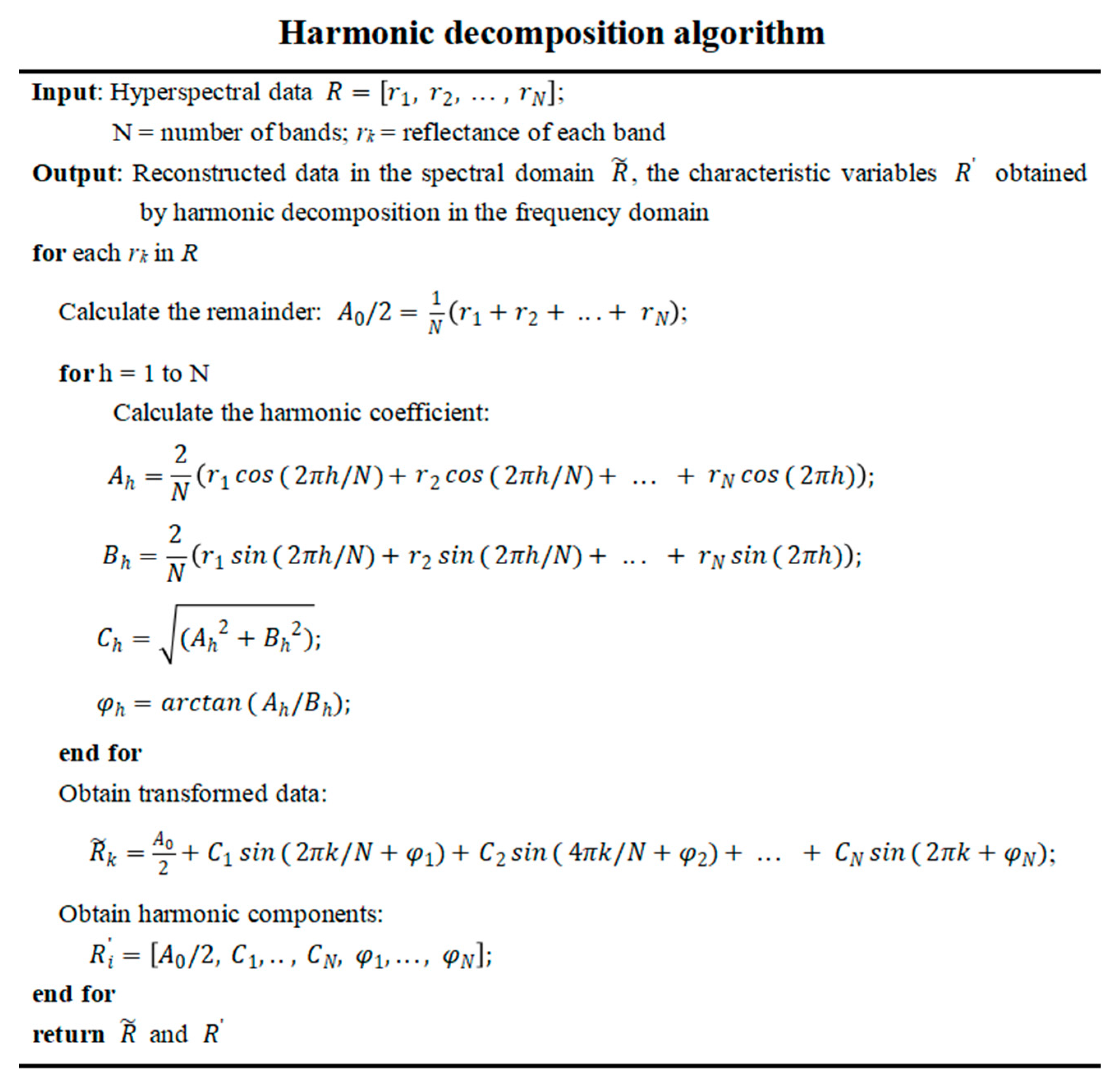
2.5. Spectral Processing Technologies

Spectral preprocessing is very useful for feature extraction and noise removal [30]. For example, WPT can perform a more detailed decomposition and reconstruction of high and low-frequency information of hyperspectral data [19]. This information processing result has no redundancy or omission, which is more conducive to spectral information noise reduction and original information retention, so it is widely used. In this research, the decomposition and reconstruction of the spectral data by WPT were performed according to the following steps.
(i)
Wavelet packet analysis. The wavelet master function used in the study was Db10 [42], by which the noise-bearing spectra were decomposed.
(ii)
Determination of the optimal wavelet packet basis. The calculation of the optimal wavelet packet basis was based on the least-cost principle.
(iii)
Wavelet packet coefficient thresholding. This process required quantization of the wavelet packet coefficients, which was based on a soft threshold “s” of good continuation.
(iv)
Spectral reconstruction. The results in (ii) and (iii) were applied to reconstruct the spectral information, and finally, the noise-reduced spectra were obtained.
Spectral measurements are susceptible to factors, such as observation angle and illumination, making the signal-to-noise ratio of spectral data comparatively poor. After differential processing, not only can the influence of changes in illumination conditions on the target spectra be reduced, but also the background can be partially eliminated, thus better strengthening the spectral variance and highlighting the target characteristics. The first-order differential (FOD) treatment can improve the spectral sensitivity and eliminate the influence of the partial environmental background to reveal the spectral characteristics of the soil interior. The FOD was calculated as follows.
Ref’(λi) = [Ref(λi+1) − Ref(λi−1)]/(λi+1λi−1),
where λi−1, λi, and λi+1 are the wavelengths of adjacent bands and Ref is the first-order differential value.
However, none of these traditional methods can obtain robust and noiseless characteristic variables. Harmonic decomposition (HD) transforms hyperspectral data from the time domain to the frequency domain in the form of sine and cosine phase superposition, and finally obtains parameters such as residual term, amplitude, and phase. The calculation method is shown in Figure 2. These variables can reveal the average value and variation of the energy, and the position of the maximum value in different bands of the spectra.

2.6. Model Construction and Validation

After the correlated characteristic variables (WF and WFH) were obtained by spectral processing technologies (WPT, FOD, and HD), they need to be dimensionally reduced to remove redundancy. The principal component analysis (PCA) method can recombine original variables into a group of new comprehensive variables unrelated to each other to achieve feature extraction and dimension reduction [43]. When performing PCA, the components whose cumulative variance contribution rate exceeds 95% of the variable is taken as the new characteristic variable in this study.
It is very important to determine the regression model based on the relationship between independent and dependent variables for accurate estimation of SMC. Principal component regression (PCR) is one of the common methods to solve the problem of collinearity in logistic regression analysis [44]. It integrates the information of variables with high correlation into the principal component with low correlation through principal component transformation and then replaces the original variable to participate in regression calculation. Partial least squares regression (PLSR) is more commonly used as a linear multiple regression analysis method [45]. By analyzing the relationship between the prediction matrix X (independent variable) and the response matrix Y (dependent variable), the initial input data are projected into a potential space, and then many potential variables are extracted by using orthogonal structure, and the linear relationship between these new variables and Y is found. This method does not directly consider the regression modeling of the dependent variable and independent variable, but comprehensively screens the information in the variable system, and selects several new components with the best explanatory ability for the system for regression modeling. Through such information screening, the noise that has no explanatory effect on the dependent variable is eliminated. Backpropagation (BP) neural network is a widely used nonlinear modeling method in the artificial neural network, which is suitable for data prediction [46]. The learning process is composed of forwarding propagation and backpropagation. In the forward propagation process, input data are gradually processed from the input layer to the output layer through the hidden layer. If the data error obtained by the output layer is not within the allowed range, the error is backpropagated and the weight of each neuron is adjusted layer by layer by the gradient descent method. Until the error meets the specified requirements, it has a better estimation effect for complex nonlinear prediction. In this paper, we choose these three methods to conduct regression modeling for spectral characteristic parameters and SMC and compare their advantages and disadvantages.
Hyperspectral estimation of SMC based on spectral processing technologies and PCA mainly includes the following four steps (Figure 3):
(i)
Data collection: preliminary investigation, spatial layout planning of soil sampling sites, and laboratory spectroscopy and SMC measurements were included.
(ii)
Data processing: the original hyperspectral data were processed by WPT, FOD, and HD, and the characteristic variables were obtained by PCA dimensionality reduction.
(iii)
Data set partitioning: 54 groups were randomly selected from 84 groups of sample data as training samples, and the other 30 groups were used as validation data to form the training and validation datasets. The SMC data description is shown in Table 2.
(iv)
Modeling and validation: PCR, PLSR, and BP were used to construct the estimation models of SMC. The coefficient of determination (R2), root mean square error (RMSE), and mean absolute error (MAE) were used to evaluate the model accuracy. Related calculations are shown as follows.
RMSE = i = 1 n ( y i y ^ i ) 2 n ,
MAE = 1 n i = 1 n | y i y i | ,
where yi is the true value, y ^ i is the predicted value, and n is the number of samples.

3. Results

3.1. Comparison of Hyperspectral Characteristics of Soils with Different SMC

Some spectral curves over the whole moisture content range were randomly selected for comparison. Hyperspectral curves of different soil types (LS, SS, and MS) are shown in Figure 4. The spectral curves of different soil types have similar shapes and the absorption characteristics of water at 1450 nm and 1960 nm dominate the spectral characteristic curves of soil. For LS, the reflectance of all observation bands generally decreases with the increase of SMC (Figure 4a). However, for SS and MS, the variation of spectral reflectance with SMC does not show a consistent variation law (Figure 4b,c). For these three different soil types, the sensitivity of spectral reflectance to SMC is low in visible and near-infrared bands, and the change is more obvious in other bands. Moreover, the characteristic of mineral absorption at 2200 nm is obvious when SMC is low but disappears gradually with the increase of SMC.

3.2. Estimation of SMC by Conventional Spectral Indices

The SMC data in the calibration set were adopted as the dependent variables, and five commonly available spectral indices (EVI, TVI, DSI, NDMI, and SARVI) were applied as independent variables to construct the inverse models using linear regression and the PLSR method, and the validation results were shown in Figure 5. The results showed that the selected spectral indices had limited accuracy in predicting the SMC of mixed soil types. Except for TVI, the remaining four indices exhibited varying degrees of overestimation or underestimation at different SMC. Although TVI did not demonstrate overestimation or underestimation (the regression line was close to the 1:1 line), the model errors were large and the points deviating from the 1:1 line were more clustered. Compared with the individual spectral indices inversion results, the PLSR model based on five indices had a higher accuracy (R2 over 0.8 and error below 4%). In addition, the model did not exhibit local overestimation or underestimation.

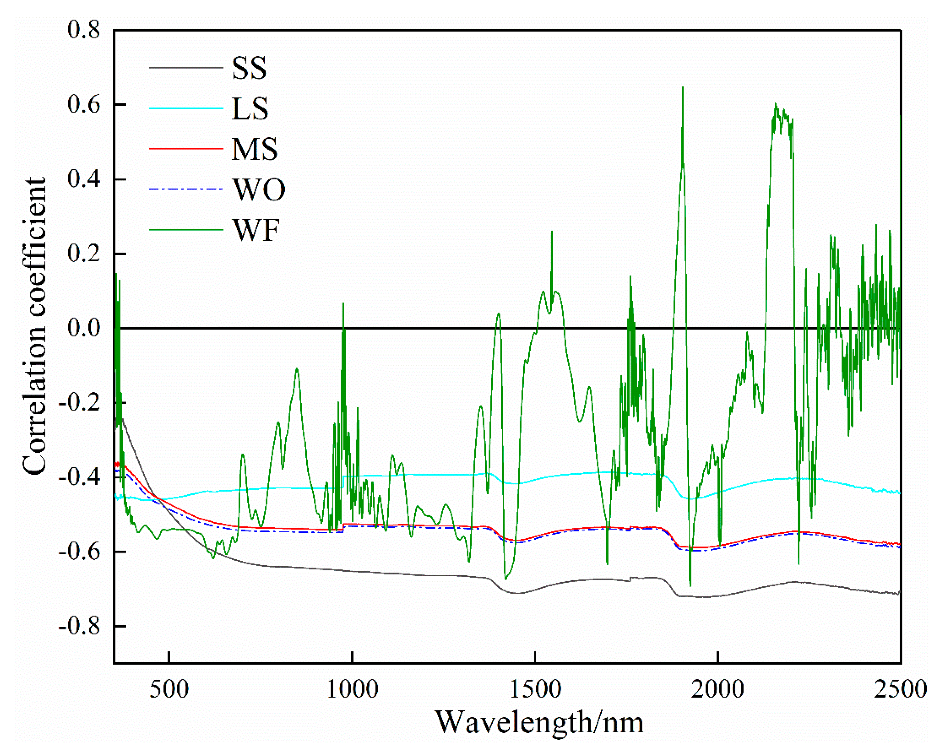
3.3. Correlation Analysis between Spectral Data and SMC

The correlation analysis between the original spectral data and the processed data of the original spectra (including WPT, FOD, and HD) and SMC was performed. The results are shown in Figure 6. SS, LS, and MS indicate the Pearson correlation coefficient (r) between the original spectra of different soil types (LS, SS, and MS) and the corresponding SMC. WO and WF represent the correlation between the WPT of original spectral data and FOD after WPT and SMC, respectively. The original spectral reflectance of SS is highly correlated with SMC except for the visible bands (|r| > 0.6, p < 0.01). The correlation between LS and SMC becomes much weaker (|r| < 0.5, p < 0.01). For MS, the correlation is between SS and LS (about 0.5, p < 0.01). Therefore, for the estimation of SMC of MS, parameters with higher correlation need to be extracted. Compared with the original spectra, WO does not significantly improve the correlation with SMC. Although WF cannot improve the correlation with SMC in all bands, it can produce parameters with a strong correlation in many characteristic bands. Finally, 180 characteristic bands were selected from WF data with |r| > 0.6 to estimate SMC.

3.4. Harmonic Characteristic Parameter Acquisition

The feature parameters of harmonic spectra (WFH: remainder, amplitude, and phase) were acquired by decomposing the selected WF data of MS. The correlation between these extracted components and SMC was computed. To keep consistent with the number of characteristic parameters of the selected WF data, the number of harmonic decompositions was determined to be 180. Figure 7 demonstrates the correlation between harmonic characteristic parameters and SMC of MS.
The result of correlation analysis reveals that the variables at the beginning and end of the decomposition numbers have a strong correlation with SMC (|r| close to 0.8, p < 0.01). The figure is roughly symmetrical in the center. Furthermore, the correlation coefficient shows a periodic change of alternating positive and negative values. Except for the beginning and the end, the correlation between other characteristic parameters close to the middle and SMC is weak (|r| < 0.5, p < 0.01). Since the correlation of characteristic parameters is periodic, half of the parameters (A0/2, Ah=1,2,4, Bh=1,2,3, C h=1,2,3, and φh=1) with high correlation with SMC (|r| > 0.7) were selected.

3.5. Dimension Reduction of Characteristic Parameters Based on PCA

After extracting the characteristic parameters through a series of spectral processing techniques (including WPT, FOD, and HD), WF and WFH data were obtained. Since many relevant characteristic parameters are included (180 of WF and 11 of WFH), it is necessary to simplify these parameters. To reduce the redundancy of variables and the input of the models, WF and WFH were processed by the PCA method, and the first five variables of the PCA results (PCA1-5) were chosen as the input characteristic variables of the SMC estimation models. The results of PCA are shown in Table 3.
It turns out that the contribution rates of cumulative variance of the first five principal components of WF and WFH were 95.915% and 99.147%, respectively. The PCA performance of WFH data is better than that of WF data. PCA1-5 of WFH data roughly includes the harmonic characteristic variable information before processing, which not only retains a large amount of original data information, but also effectively compresses the original data. According to all PCA results, two characteristic variables were established: WFP (PCA of WF) and WFHP (PCA of WFH).

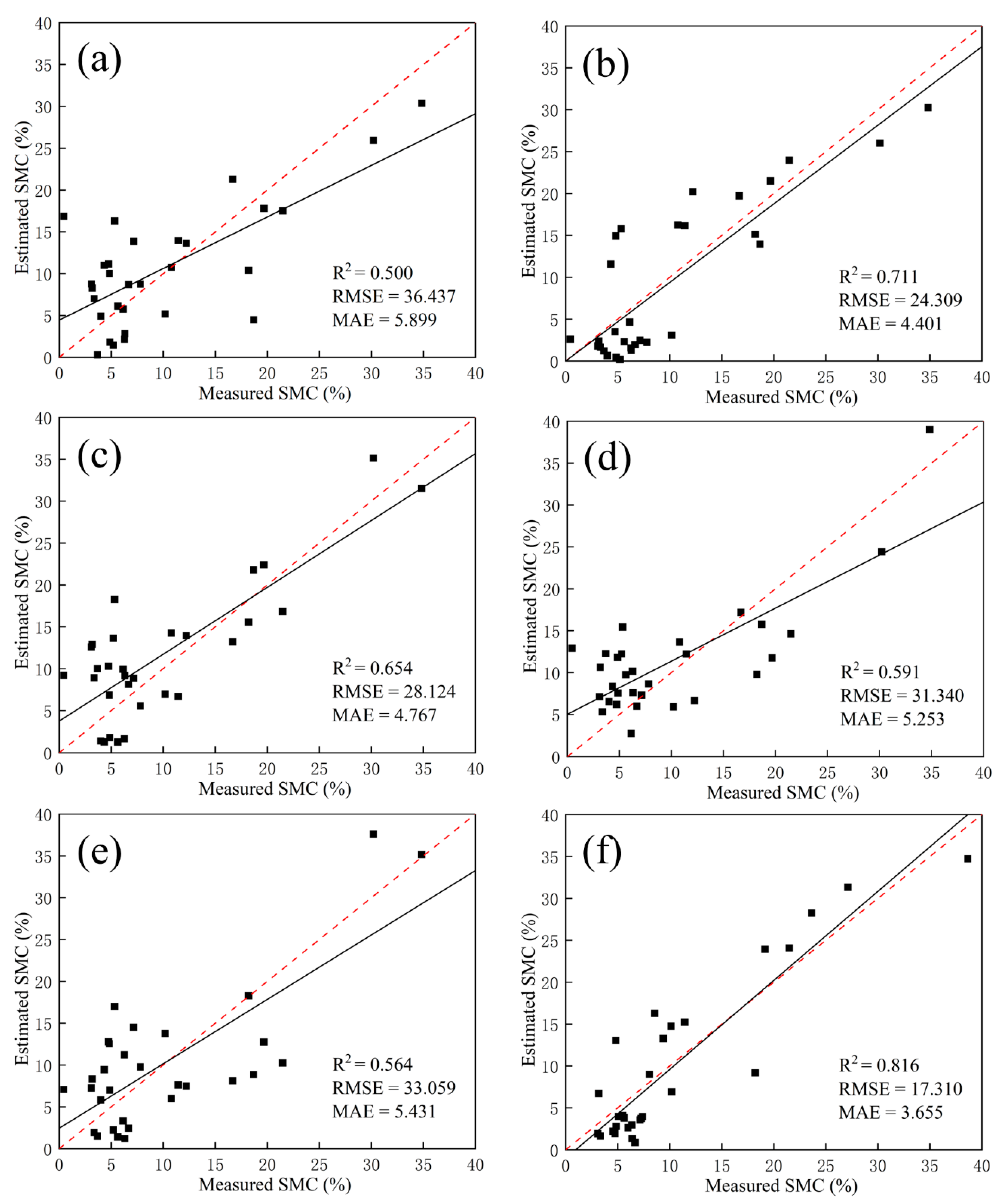
3.6. SMC Estimation and Model Validation Using Spectral Processing Technologies and Harmonic Indicators

Three regression estimation models (PCR, BP, and PLSR) were selected to explore the validity of characteristic variables and the accuracy of the soil moisture estimation models. Based on the modeling of WFP and WFHP, six SMC prediction models were established: WFP-PCR, WFHP-PCR, WFP-BP, WFHP-BP, WFP-PLSR, and WFHP-PLSR. For the BP neural network model, the topology of the model was finally determined as 5-3-1 after several debugging. That is, the number of nodes in the input layer is 5, the number of hidden layers is 5, and the output result layer is 1. Meanwhile, the times of iterations, adaptive learning rate, momentum factor, and the learning error were set as 3000, 0.01, 0.9, and 0.001, respectively. The precision and error of the modeling set and validation set are shown in Table 4. The WFHP has better performance than WFP for the PCR, PLSR, and BP models in calibration and validation datasets. For the same regression model, BP neural network has the highest accuracy than PCR and PLSR. In all similar models, the accuracy of the validation set is slightly lower than that of the modeling set.
To further observe the effect of different variables and different methods on the estimation of different SMC, the scatter diagram of the estimated and measured value of SMC in the validation dataset is shown in Figure 8. Each row represents different regression models of similar characteristic variables (WFP or WFHP), and each column represents the same regression model of different characteristic variables (PCR, PLSR, or BP). The red dotted line indicates the 1:1 line. It can be found that the WFP-based models are prone to underestimation when the SMC exceeds 10% (below the 1:1 line), while the WFHP-based models can accurately estimate SMC in the whole range (almost overlaps with the 1:1 line). For the same characteristic variable, the effect of PLSR and BP is significantly better than that of PCR (closer to the 1:1 line).
Compared with the traditional spectral indices prediction results (Figure 5), the validation accuracy of all models, except the WFP-PCR model, was higher with an error below 3% (Table 4 and Figure 8). This indicated that there was a great potential for spectral variables based on spectral processing techniques upon SMC estimation for mixed soil types.

4. Discussion

Traditional soil moisture measurements using neutron scattering, drying method, and resistance method have been part of many agricultural studies [47,48,49]. While these measurements provide accurate results, they are tedious, time consuming, and laborious, making it difficult to scale in large areas [50]. Compared with traditional soil moisture monitoring methods, remote sensing has incomparable advantages such as a large area and being a macroscopic, real-time, and dynamic method [30]. The hyperspectral sensor can detect the subtle changes in surface characteristics, and hyperspectral quantitative inversion provides an effective technical means for dynamic monitoring of regional SMC [9,19]. However, obtaining the best characteristic variables of SMC estimation of mixed soil types has always been difficult in modeling. In SMC estimation, the original soil spectral reflectance data contain much noise and a lot of redundant information, which cannot be used directly to estimate SMC. There are many differences in spectral characteristics of different soil types. For example, in SS spectral analysis, the reflectance of all bands decreases with the increase of SMC overall (Figure 4), showing a strong negative correlation (Figure 5). In LS, except for SMC, the variation rule of reflectance is not obvious due to the difference in organic matter content, grain size distribution, mineral composition, and soil color [51], thus reducing the correlation with SMC. However, the small content of these substances in SS has a small impact on reflectance. Therefore, it is difficult to establish a general SMC estimation model. In most cases, it is necessary to carry out the spectral transformation on the original soil spectral reflection data, such as reciprocal, logarithm, FOD, etc. to extract characteristic bands or parameters to obtain feature variables [52]. However, these methods have a low noise reduction function and cannot deal with data background and noise well, which directly affects the accuracy of subsequent estimation.
In this paper, the results of several traditional spectral indices for estimating SMC showed that both univariate linear regression models and multivariate PLSR models had significant errors. Therefore, it is necessary to explore the variables and methods for SMC estimation in mixed soil types.
Through correlation analysis, it can be found that the correlation between WF and SMC is significantly higher than that of the original spectra and SMC (Figure 6). It shows that the FOD spectra can eliminate some effects of background and atmosphere, but still cannot achieve satisfactory results. In this paper, the HD method was adopted. The soil spectra were converted to frequency spectra to obtain harmonic characteristic parameters based on Fourier transform theory to effectively reduce the uncertainty of spectral parameter calculation. Furthermore, harmonic parameters can better reflect soil spectral changes caused by subtle changes in soil internal components. Compared with traditional spectral parameters, harmonic characteristic parameters (remainder, amplitude, and phase) are more correlated with SMC (Figure 7). Finally, 11 harmonic characteristic parameters with high correlation (|r| > 0.7) were selected. Based on the FOD and HD, the PCA method was applied to reduce the dimensionality of data and two kinds of feature parameters were gained: WFP and WFHP.
In parameter estimation studies using empirical models, PLSR, BP, and PCR all showed good effects [16,28,30]. To explore the applicability of the two types of characteristic parameters extracted in this paper (WFP and WFHP), these three models were used for comparison of estimation. The results show that WFPH is superior to WFP in SMC estimation in these three models (Table 4 and Figure 8). When selecting the same characteristic parameters (WFP or WFHP), the effects of PLSR and BP models are significantly better than PCR. The advantage of the PLSR model is that it can strengthen the error convergence ability of the model when the sample size is not particularly sufficient, while BP is a nonlinear distribution that can better reflect SMC and is mainly good at nonlinear prediction. Soil spectra are a comprehensive reflection of various soil properties, and the selection of estimation model alone cannot effectively solve the problem of accurate estimation of SMC. Therefore, it is necessary to explore some common and stable characteristic parameters to establish a more robust and suitable SMC inversion model. The harmonic characteristic parameters constructed in this paper can transform complex signals in the time domain into simplified signals in the frequency domain, which can not only suppress or eliminate ground object background noise, but also highlight the spectral characteristics of the ground object with low order harmonic components to achieve the effect of data compression. Therefore, the SMC prediction ability of the three models (BP, PLSR, and PCR) was effectively improved. Moreover, the advantage of harmonic variables in predicting SMC also reflects that they can accurately predict different SMC, including low and high values, while WFP parameters are underestimated at high values of SMC (Figure 8).
To further check the performance of the optimal model (WFHP-BP) in this paper for SMC estimation in different soil types, the validation models for single soil types are shown in Figure 9. It can be found that the estimation accuracy of SMC is better than that of mixed soil types in both SS and LS, and neither of them shows local overestimation and underestimation. This may be because single soil types are more consistent physically or chemically and thus receive less interference from other factors. Since the BP neural network model has a nonlinear learning capability, the estimated values of SMC for different soil types did not appear to be overestimated or underestimated.
This study provided effective parameters and methods for nondestructive estimation of SMC in mixed soil types, and future research should be devoted to using satellite imagery as an alternative to ground-based measurements because of its large area, economy, time savings, and high temporal resolution, which can provide a data source for real-time field SMC mapping.

5. Conclusions

In this paper, a feature extraction method based on spectral processing technologies (WPT, FOD, and HD) and PCA was proposed, and three regression prediction methods (PCR, PLSR, and BP) were combined to compare the accuracy and applicability of SMC estimation for mixed soil. It is observed that for SS with less impurity, the variation of spectral reflectance can well describe the difference in SMC. However, for LS and MS, the spectral reflectance cannot be directly used to predict the SMC due to the influence of organic matter content, grain size distribution, mineral composition, and soil color. After WPT and FOD transformation using the original spectral data, two sets of data can be obtained after HD: WF and WFH. Meanwhile, the PCA method was utilized to reduce the dimensionality of these two datasets to obtain two sets of characteristic parameters: WFP and WFHP. The results of three regression models (WFP-PCR, WFHP-PCR, WFP-PLSR, WFHP-PLSR, WFP-BP, and WFHP-BP) indicated that the WFHP-based models showed better performance than that of WFP-based models. Among the different regression methods, BP neural network has the highest accuracy as a result of its nonlinear prediction ability. The best prediction model is WFHP-BP (R2 = 0.932, RMSE = 2.311, MAE = 1.834 for the validation dataset). Moreover, harmonic variables have advantages in predicting SMC values in a larger range. This study can provide a theoretical basis and technical support for establishing SMC inversion models suitable for various types and a large range of soils. Future research should focus more on the use of satellite remote sensing data and on proposing physical or chemical indicators of soils that are more suitable for SMC estimation.

Author Contributions

Conceptualization, S.L. and X.J.; methodology, X.J.; software, S.L.; validation, Q.Y.; writing—original draft preparation, X.J. and S.L.; writing—review and editing, X.L.; visualization, W.J.; funding acquisition, Q.Y. All authors have read and agreed to the published version of the manuscript.

Funding

This research was funded by the National Natural Science Foundation of China (Grant No.52078350), the National Key Research and Development Program of China (Grant No.2018YFB0505400), and the Natural Science Foundation of Shanghai (Grant No.22ZR1465700).

Institutional Review Board Statement

Not applicable.

Informed Consent Statement

Not applicable.

Data Availability Statement

Not applicable.

Conflicts of Interest

The authors declare no conflict of interest.

References

  1. Ebtehaj, A.; Bras, R.L. A physically constrained inversion for high-resolution passive microwave retrieval of soil moisture and vegetation water content in L-band. Remote Sens. Environ. 2019, 233, 15. [Google Scholar] [CrossRef]
  2. Bablet, A.; Viallefont-Robinet, F.; Jacquemoud, S.; Fabre, S.; Briottet, X. High-resolution mapping of in-depth soil moisture content through a laboratory experiment coupling a spectroradiometer and two hyperspectral cameras. Remote Sens. Environ. 2020, 236, 11. [Google Scholar] [CrossRef]
  3. Arunrat, N.; Sereenonchai, S.; Hatano, R. Effects of fire on soil organic carbon, soil total nitrogen, and soil properties under rotational shifting cultivation in northern Thailand. J. Environ. Manag. 2022, 302, 15. [Google Scholar] [CrossRef] [PubMed]
  4. Qu, W.D.; Han, G.X.; Wang, J.; Li, J.Y.; Zhao, M.L.; He, W.J.; Li, X.G.; Wei, S.Y. Short-term effects of soil moisture on soil organic carbon decomposition in a coastal wetland of the Yellow River Delta. Hydrobiologia 2021, 848, 3259–3271. [Google Scholar] [CrossRef]
  5. Gibon, F.; Pellarin, T.; Roman-Cascon, C.; Alhassane, A.; Traore, S.; Kerr, Y.; Lo Seen, D.; Baron, C. Millet yield estimates in the Sahel using satellite derived soil moisture time series. Agric. For. Meteorol. 2018, 262, 100–109. [Google Scholar] [CrossRef]
  6. Humphrey, V.; Berg, A.; Ciais, P.; Gentine, P.; Jung, M.; Reichstein, M.; Seneviratne, S.I.; Frankenberg, C. Soil moisture-atmosphere feedback dominates land carbon uptake variability. Nature 2021, 592, 65–69. [Google Scholar] [CrossRef]
  7. Liu, L.B.; Gudmundsson, L.; Hauser, M.; Qin, D.H.; Li, S.C.; Seneviratne, S.I. Soil moisture dominates dryness stress on ecosystem production globally. Nat. Commun. 2020, 11, 9. [Google Scholar] [CrossRef]
  8. Sadeghi, M.; Jones, S.B.; Philpot, W.D. A linear physically-based model for remote sensing of soil moisture using short wave infrared bands. Remote Sens. Environ. 2015, 164, 66–76. [Google Scholar] [CrossRef]
  9. Zhang, Y.; Tan, K.; Wang, X.; Chen, Y. Retrieval of soil moisture content based on a modified Hapke Photometric model: A novel method applied to laboratory hyperspectral and Sentinel-2 MSI data. Remote Sens. 2020, 12, 2239. [Google Scholar] [CrossRef]
  10. Luo, C.; Zhang, X.L.; Meng, X.T.; Zhu, H.W.; Ni, C.P.; Chen, M.H.; Liu, H.J. Regional mapping of soil organic matter content using multitemporal synthetic Landsat 8 images in Google Earth Engine. Catena 2022, 209, 11. [Google Scholar] [CrossRef]
  11. Niyogi, D.; Jamshidi, S.; Smith, D.; Kellner, O. Evapotranspiration climatology of Indiana using in situ and remotely sensed products. J. Appl. Meteorol. Climatol. 2020, 59, 2093–2111. [Google Scholar] [CrossRef]
  12. Jamshidi, S.; Zand-Parsa, S.; Niyogi, D. Assessing crop water stress index of citrus using in-situ measurements, Landsat, and Sentinel-2 data. Int. J. Remote Sens. 2021, 42, 1893–1916. [Google Scholar] [CrossRef]
  13. Skakun, S.; Kalecinski, N.I.; Brown, M.G.L.; Johnson, D.M.; Vermote, E.F.; Roger, J.C.; Franch, B. Assessing within-field corn and soybean yield variability from WorldView-3, Planet, Sentinel-2, and Landsat 8 satellite imagery. Remote Sens. 2021, 13, 872. [Google Scholar] [CrossRef]
  14. Eon, R.S.; Bachmann, C.M. Mapping barrier island soil moisture using a radiative transfer model of hyperspectral imagery from an unmanned aerial system. Sci. Rep. 2021, 11, 11. [Google Scholar] [CrossRef] [PubMed]
  15. Muller, E.; Decamps, H. Modeling soil moisture-reflectance. Remote Sens. Environ. 2001, 76, 173–180. [Google Scholar] [CrossRef] [Green Version]
  16. Pellegrini, E.; Rovere, N.; Zaninotti, S.; Franco, I.; De Nobili, M.; Contin, M. Artificial neural network (ANN) modelling for the estimation of soil microbial biomass in vineyard soils. Biol. Fertil. Soils 2021, 57, 145–151. [Google Scholar] [CrossRef]
  17. Emamgholizadeh, S.; Mohammadi, B. New hybrid nature-based algorithm to integration support vector machine for prediction of soil cation exchange capacity. Soft Comput. 2021, 25, 13451–13464. [Google Scholar] [CrossRef]
  18. Yin, Z.; Lei, T.W.; Yan, Q.H.; Chen, Z.P.; Dong, Y.Q. A near-infrared reflectance sensor for soil surface moisture measurement. Comput. Electron. Agric. 2013, 99, 101–107. [Google Scholar] [CrossRef]
  19. Jiang, X.Q.; Luo, S.J.; Fang, S.H.; Cai, B.W.; Xiong, Q.; Wang, Y.Y.; Huang, X.; Liu, X.J. Remotely sensed estimation of total iron content in soil with harmonic analysis and BP neural network. Plant Methods 2021, 17, 12. [Google Scholar] [CrossRef]
  20. Cheng, H.; Wang, J.; Du, Y.K.; Zhai, T.L.; Fang, Y.; Li, Z.H. Exploring the potential of canopy reflectance spectra for estimating organic carbon content of aboveground vegetation in coastal wetlands. Int. J. Remote Sens. 2021, 42, 3850–3872. [Google Scholar] [CrossRef]
  21. Li, Y.; Via, B.K.; Li, Y.X. Lifting wavelet transform for Vis-NIR spectral data optimization to predict wood density. Spectroc. Acta Pt. A-Molec. Biomolec. Spectr. 2020, 240, 9. [Google Scholar] [CrossRef] [PubMed]
  22. Luo, S.J.; He, Y.B.; Wang, Z.Z.; Duan, D.D.; Zhang, J.K.; Zhang, Y.T.; Zhu, Y.Q.; Yu, J.K.; Zhang, S.L.; Xu, F.; et al. Comparison of the retrieving precision of potato leaf area index derived from several vegetation indices and spectral parameters of the continuum removal method. Eur. J. Remote Sens. 2019, 52, 155–168. [Google Scholar] [CrossRef] [Green Version]
  23. Blanco, M.; Coello, J.; Iturriaga, H.; Maspoch, S.; Pages, J. NTR calibration in non-linear systems: Different PLS approaches and artificial neural networks. Chemometrics Intell. Lab. Syst. 2000, 50, 75–82. [Google Scholar] [CrossRef]
  24. Gu, X.H.; Wang, Y.C.; Sun, Q.; Yang, G.J.; Zhang, C. Hyperspectral inversion of soil organic matter content in cultivated land based on wavelet transform. Comput. Electron. Agric. 2019, 167, 7. [Google Scholar] [CrossRef]
  25. Yuan, L.N.; Li, L.; Zhang, T.; Chen, L.Q.; Liu, W.Q.; Hu, S.; Yang, L.H. Modeling Soil Moisture from Multisource Data by Stepwise Multilinear Regression: An Application to the Chinese Loess Plateau. ISPRS Int. J. Geo-Inf. 2021, 10, 233. [Google Scholar] [CrossRef]
  26. Xiong, J.F.; Lin, C.; Ma, R.H.; Zheng, G.H. The total P estimation with hyper-spectrum A novel insight into different P fractions. Catena 2020, 187, 11. [Google Scholar] [CrossRef]
  27. Lin, N.; Liu, H.Q.; Yang, J.J.; Liu, H.L. Hyperspectral estimation of soil composition contents based on kernel principal component analysis and machine learning model. J. Appl. Remote Sens. 2020, 14, 19. [Google Scholar] [CrossRef]
  28. Yang, J.C.; Wang, X.L.; Wang, R.H.; Wang, H.J. Combination of convolutional neural networks and recurrent neural networks for predicting soil properties using Vis-NIR spectroscopy. Geoderma 2020, 380, 16. [Google Scholar] [CrossRef]
  29. Taghizadeh-Mehrjardi, R.; Schmidt, K.; Toomanian, N.; Heung, B.; Behrens, T.; Mosavi, A.; Band, S.S.; Amirian-Chakan, A.; Fathabadi, A.; Scholten, T. Improving the spatial prediction of soil salinity in arid regions using wavelet transformation and support vector regression models. Geoderma 2021, 383, 21. [Google Scholar] [CrossRef]
  30. Shen, L.Z.; Gao, M.F.; Yan, J.W.; Li, Z.L.; Leng, P.; Yang, Q.; Duan, S.B. Hyperspectral estimation of soil organic matter content using different spectral preprocessing techniques and PLSR method. Remote Sens. 2020, 12, 1206. [Google Scholar] [CrossRef] [Green Version]
  31. Ma, Y.; Fang, S.H.; Peng, Y.; Gong, Y.; Wang, D. Remote estimation of biomass in winter oilseed rape (Brassica napus L.) using canopy hyperspectral data at different growth stages. Appl. Sci. 2019, 9, 545. [Google Scholar] [CrossRef] [Green Version]
  32. Tian, H.R.; Wang, P.X.; Tansey, K.; Zhang, S.Y.; Zhang, J.Q.; Li, H.M. An IPSO-BP neural network for estimating wheat yield using two remotely sensed variables in the Guanzhong Plain, PR China. Comput. Electron. Agric. 2020, 169, 10. [Google Scholar] [CrossRef]
  33. Shi, Y.J.; Ren, C.; Yan, Z.H.; Lai, J.M. High spatial-temporal resolution estimation of ground-based global navigation satellite system interferometric reflectometry (GNSS-IR) soil moisture using the genetic algorithm back propagation (GA-BP) neural network. ISPRS Int. J. Geo-Inf. 2021, 10, 623. [Google Scholar] [CrossRef]
  34. Wang, X.; An, S.; Xu, Y.Q.; Hou, H.P.; Chen, F.Y.; Yang, Y.J.; Zhang, S.L.; Liu, R. A back propagation neural network model optimized by mind evolutionary algorithm for estimating Cd, Cr, and Pb concentrations in soils using Vis-NIR diffuse reflectance spectroscopy. Appl. Sci. 2020, 10, 51. [Google Scholar] [CrossRef] [Green Version]
  35. Liang, Y.J.; Ren, C.; Wang, H.Y.; Huang, Y.B.; Zheng, Z.T. Research on soil moisture inversion method based on GA-BP neural network model. Int. J. Remote Sens. 2019, 40, 2087–2103. [Google Scholar] [CrossRef]
  36. Dong, Z.Q.; Liu, Y.; Ci, B.X.; Wen, M.; Li, M.H.; Lu, X.; Feng, X.K.; Wen, S.; Ma, F.Y. Estimation of nitrate nitrogen content in cotton petioles under drip irrigation based on wavelet neural network approach using spectral indices. Plant Methods 2021, 17, 13. [Google Scholar] [CrossRef]
  37. Tao, L.L.; Wang, G.J.; Chen, X.; Li, J.; Cai, Q.K. Soil moisture retrieval using modified particle swarm optimization and back-propagation neural network. Photogramm. Eng. Remote Sens. 2019, 85, 789–798. [Google Scholar] [CrossRef]
  38. Kahaer, Y.; Tashpolat, N.; Shi, Q.D.; Liu, S.H. Possibility of Zhuhai-1 hyperspectral imagery for monitoring salinized soil moisture content using fractional order differentially optimized spectral indices. Water 2020, 12, 3360. [Google Scholar] [CrossRef]
  39. Li, X.; Ding, J.L. Soil moisture monitoring based on measured hyperspectral index and HSI image index. Trans. Chin. Soc. Agric. Eng. 2015, 31, 68–75. [Google Scholar] [CrossRef]
  40. Zhang, X.L.; Zhang, F.; Zhang, H.W.; Li, Z.; Hai, Q.; Chen, L.H. Optimization of soil salt inversion model based on spectral transformation from hyperspectral index. Trans. Chin. Soc. Agric. Eng. 2018, 34, 110–117. [Google Scholar] [CrossRef]
  41. Liu, Y.; Pan, X.Z.; Wang, C.K.; Li, Y.L.; Shi, R.J.; Li, Z.T. Prediction of saline soil moisture content based on differential spectral index: A case study of coastal saline soil. Soils 2016, 48, 381–388. [Google Scholar] [CrossRef]
  42. Wu, D.H.; Fan, W.J.; Cui, Y.K.; Yan, B.Y.; Xu, X.R. Review of monitoring soil water content using hyperspectral remote sensing. Spectrosc. Spectr. Anal. 2010, 30, 3067–3071. [Google Scholar] [CrossRef]
  43. Tripathi, M.; Singal, S.K. Use of principal component analysis for parameter selection for development of a novel water quality index: A case study of river Ganga India. Ecol. Indic. 2019, 96, 430–436. [Google Scholar] [CrossRef]
  44. Fernandez-Delgado, M.; Cernadas, E.; Barro, S.; Amorim, D. Do we need hundreds of classifiers to solve real world classification problems? J. Mach. Learn. Res. 2014, 15, 3133–3181. [Google Scholar]
  45. Meacham-Hensold, K.; Montes, C.M.; Wu, J.; Guan, K.Y.; Fu, P.; Ainsworth, E.A.; Pederson, T.; Moore, C.E.; Brown, K.L.; Raines, C.; et al. High-throughput field phenotyping using hyperspectral reflectance and partial least squares regression (PLSR) reveals genetic modifications to photosynthetic capacity. Remote Sens. Environ. 2019, 231, 10. [Google Scholar] [CrossRef]
  46. Sun, W.; Huang, C.C. A carbon price prediction model based on secondary decomposition algorithm and optimized back propagation neural network. J. Clean Prod. 2020, 243, 13. [Google Scholar] [CrossRef]
  47. Dominguez-Nino, J.M.; Oliver-Manera, J.; Girona, J.; Casadesus, J. Differential irrigation scheduling by an automated algorithm of water balance tuned by capacitance-type soil moisture sensors. Agric. Water Manag. 2020, 228, 11. [Google Scholar] [CrossRef]
  48. Jamshidi, S.; Zand-Parsa, S.; Niyogi, D. Physiological responses of orange trees subject to regulated deficit irrigation and partial root drying. Irrig. Sci. 2021, 39, 441–455. [Google Scholar] [CrossRef]
  49. Jamshidi, S.; Zand-Parsa, S.; Kamgar-Haghighi, A.A.; Shahsavar, A.R.; Niyogi, D. Evapotranspiration, crop coefficients, and physiological responses of citrus trees in semi-arid climatic conditions. Agric. Water Manag. 2020, 227, 12. [Google Scholar] [CrossRef]
  50. Wu, T.H.; Yu, J.; Lu, J.X.; Zou, X.G.; Zhang, W.T. Research on inversion model of cultivated soil moisture content based on hyperspectral imaging analysis. Agriculture 2020, 10, 292. [Google Scholar] [CrossRef]
  51. Jacquemoud, S.; Baret, F.; Hanocq, J.F. Modeling spectral and bidirectional soil reflectance. Remote Sens. Environ. 1992, 41, 123–132. [Google Scholar] [CrossRef]
  52. Tian, A.H.; Zhao, J.S.; Tang, B.H.; Zhu, D.M.; Fu, C.B.; Xiong, H.G. Hyperspectral prediction of soil total salt content by different disturbance degree under a fractional-order differential model with differing spectral transformations. Remote Sens. 2021, 13, 4283. [Google Scholar] [CrossRef]
Figure 1. Study region and soil sampling area (the blue dots show the sampling areas).
Agriculture 12 01188 g001
Figure 2. Illustration of the harmonic decomposition algorithm in pseudo-code.
Agriculture 12 01188 g002
Figure 3. Flowchart indicating experimental methodology (WPT: wavelet packet transform; FOD: first-order differential; HD: harmonic decomposition; WFP: WPT-FOD-PCA; WFHP: WPT-FOD-HD-PCA).
Agriculture 12 01188 g003
Figure 4. Hyperspectral curves of different soil types: (a) LS; (b) SS; (c) MS.
Agriculture 12 01188 g004
Figure 5. The comparison of measured and estimated SMC: (a) EVI; (b) TVI; (c) DSI; (d) NDMI; (e) SARVI; (f) PLSR model of five spectral indices.
Agriculture 12 01188 g005
Figure 6. The Pearson correlation coefficient between spectra and SMC.
Agriculture 12 01188 g006
Figure 7. The Pearson correlation coefficient between harmonic characteristic parameters and SMC.
Agriculture 12 01188 g007
Figure 8. The comparison of measured and estimated SMC: (a) WFP-PCR; (b) WFP-PLSR; (c) WFP-BP; (d) WFHP-PCR; (e) WFHP-PLSR; (f) WFHP-BP.
Agriculture 12 01188 g008
Figure 9. The comparison of measured and estimated SMC of different types of soil.
Agriculture 12 01188 g009
Table 1. The common spectral indices selected in this paper.
Spectral IndicesFormulaReference
EVI 2.5 ( R 1828 R 630 ) R 1828 + 6 R 630 7.5 R 450 + 1 [39]
TVI0.5[120(R666 − R834) − 200(R794 − R834)][38]
DSIR1760 − R1715[40]
NDMI R 2027 R 1878 R 2027 + R 1878 [41]
SARVI 1.5 ( R 1820 R 670 ) R 1820 + R 670 + 0.5 [39]
Table 2. Descriptive statistics of SMC in soils.
Soil TypesSamplesSMC (%)
MinMaxMeanSDCV(%)
Loessial soil513.3658.439.658.0583.40
Sandy soil330.4638.6512.0911.0391.18
Training data542.0958.4310.9910.0291.14
Validation data300.4634.8310.728.8782.74
Mixed soil840.4658.4310.899.6288.34
Table 3. The PCA results in eigenvalue and variance contribution rate.
PCAEigenvalueVariance Contribution (%)Accumulative Contribution (%)
WFWFHWFWFHWFWFH
PCA1927.6 × 10−80.075689.74294.27989.74294.279
PCA240.8 × 10−84.613 × 10−83.2163.45792.95897.736
PCA316.55 × 10−81.572 × 10−91.7621.25394.72098.989
PCA410.17 × 10−81.396 × 10−100.9650.10295.68599.091
PCA59.36 × 10−81.631 × 10−100.2300.05695.91599.147
Table 4. Accuracy comparison of different regression models.
ModelCalibrationValidation
R2RMSE (%)MAE (%)R2RMSE (%)MAE (%)
WFP-PCR0.8123.6933.3630.7634.2613.771
WFHP-PCR0.8513.2792.8190.8363.5232.902
WFP-PLSR0.8822.9772.6320.8633.0862.759
WFHP-PLSR0.9022.6732.6010.9072.8262.583
WFP-BP0.9172.5042.1320.9092.6262.286
WFHP-BP0.9452.1151.6530.9322.3111.834
Publisher’s Note: MDPI stays neutral with regard to jurisdictional claims in published maps and institutional affiliations.

