Article

Monitoring Maize Growth and Calculating Plant Heights with Synthetic Aperture Radar (SAR) and Optical Satellite Images

1
Remote Sensing and Geographic Information Systems Graduate Program, Institute of Natural and Applied Sciences, Akdeniz University, Antalya 07058, Turkey
2
Department of Agricultural Machinery and Technologies Engineering, Faculty of Agriculture, Akdeniz University, Antalya 07058, Turkey
3
Department of Space Sciences and Technologies, Faculty of Science, Akdeniz University, Antalya 07058, Turkey
*
Author to whom correspondence should be addressed.
Agriculture 2022, 12(6), 800; https://doi.org/10.3390/agriculture12060800
Submission received: 23 April 2022 / Revised: 28 May 2022 / Accepted: 30 May 2022 / Published: 1 June 2022

Abstract

:
The decrease in water resources due to climate change is expected to have a significant impact on agriculture. On the other hand, as the world population increases so does the demand for food. It is necessary to better manage environmental resources and maintain an adequate level of crop production in a world where the population is constantly increasing. Therefore, agricultural activities must be closely monitored, especially in maize fields since maize is of great importance to both humans and animals. Sentinel-1 Synthetic Aperture Radar (SAR) and Sentinel-2 optical satellite images were used to monitor maize growth in this study. Backscatter and interferometric coherence values derived from Sentinel-1 images, as well as Normalized Difference Vegetation Index (NDVI) and values related to biophysical variables (such as Leaf Area Index (LAI), Fraction of Vegetation Cover (fCover or FVC), and Canopy Water Content (CW)) derived from Sentinel-2 images were investigated. Sentinel-1 images were also used to calculate plant heights. The Interferometric SAR (InSAR) technique was applied to calculate interferometric coherence values and plant heights. For the plant height calculation, two image pairs with the largest possible perpendicular baseline were selected. Backscatter, NDVI, LAI, fCover, and CW values were low before planting, while the interferometric coherence values were generally high. Backscatter, NDVI, LAI, fCover, and CW values increased as the maize grew, while the interferometric coherence values decreased. Among all Sentinel-derived values, fCover had the best correlation with maize height until maize height exceeded 260 cm (R2 = 0.97). After harvest, a decrease in backscatter, NDVI, LAI, fCover, and CW values and an increase in interferometric coherence values were observed. NDVI, LAI, fCover, and CW values remained insensitive to tillage practices, whereas backscatter and interferometric coherence values were found to be sensitive to planting operations. In addition, backscatter values were also sensitive to irrigation operations, even when the average maize height was about 235 cm. Cloud cover and/or fog near the study area were found to affect NDVI, LAI, fCover, and CW values, while precipitation events had a significant impact on backscatter and interferometric coherence values. Furthermore, using Sentinel-1 images, the average plant height was calculated with an error of about 50 cm.

1. Introduction

Maize (Zea mays L.) is used as a raw material in the production of biofuels and other industrial products in addition to being used as human food and animal feed [1]. Maize is one of the most important crops in the world [2,3] and therefore it is widely cultivated [4] due to these characteristics. It is so popular that it is the most widely produced [5] and demanded grain on the planet [6]. Maize, which is a very important crop in Turkey as well, is the third grain with the largest cultivation area and the highest production amount in Turkey after wheat and barley [7]. Therefore, monitoring maize growth is critical [4], since it is crucial for national food security [1,4].
The soil and crop conditions in agricultural areas change from day to day [8,9] and throughout the growing season [9,10]; therefore, agricultural areas must be monitored throughout the entire growing season [9]. Traditional ground-based monitoring activities to obtain information on soil and crop conditions are time consuming and expensive. Thus, it is difficult to use this method throughout the growing season. Furthermore, the data obtained using this method do not provide information about the field’s spatial distribution. For this reason, this method is rarely used in large-scale studies [11]. The remote sensing technique, on the other hand, saves time and money [12] and enables large-scale [11,13], timely [14], and accurate monitoring of agricultural areas throughout the growing season.
Agricultural applications such as crop planting areas determination, crop growth monitoring, crop type mapping, biomass, and yield estimation are generally done with optical images, due to the data’s ease of interpretation [14]. Vegetation indices and biophysical variables values derived from optical data are commonly used to monitor agricultural areas. NDVI, e.g., [15,16,17], which is one of the most widely used vegetation indices [15,18], and LAI [17,19], which is one of the most widely used biophysical variables, have been frequently used to monitor maize growth in previous studies. Furthermore, some studies have reported that crop growth can be monitored more effectively by including less frequently used vegetation indices [20,21].
On the other hand, crop growth is a dynamic process [22]. To monitor crop growth, regular remote sensing measurements are required [23]. Cloud cover, fog, and smoke hinder passive optical sensors from getting information about the earth’s surface [24]. Given that the majority of the world is cloud-covered [25], obtaining optical satellite images with high spatial and temporal resolution throughout the growing season is extremely difficult [26], particularly in agricultural areas located in humid and semi-humid climatic zones with plentiful water resources and dense cloud cover [27]. Active SAR sensors, unlike optical sensors, can obtain high spatial and temporal resolution images in all weather conditions, day and night [2,28]. Due to these features, SAR data has an important advantage for monitoring agricultural areas [29,30,31].
The use of SAR data in agricultural applications has increased in recent years and many studies have been conducted to monitor maize growth using backscatter values, e.g., [10,29,30,32]. McNairn et al. [29] found that C-band HH-polarized backscatter values were sensitive to changes in maize height at early growth stages, but became insensitive to changes in maize height when the backscatter values achieved saturation once the maize height exceeded 1 m. Abdikan et al. [33] observed a strong correlation between SAR backscatter derived from Sentinel-1 images and maize height until the maize height exceeded 150 cm, after which the sensitivity of SAR backscatter to maize height reduced. On the other hand, McNairn et al. [34] reported that backscatter values were insensitive to changes in maize growth.
While the spectrum characteristics of the agricultural targets [14], specifically their reflection and emission qualities [35], are crucial in optical remote sensing, geometric and dielectric properties of the agricultural targets [14,27,36,37,38] such as their surface roughness, water/moisture content, plant density, canopy structure, and row direction [37] are crucial in SAR remote sensing. SAR backscatter is affected by a variety of factors, therefore the effect of soil and vegetation on backscatter is poorly understood [39] and data on vegetation are difficult to extract [40]. In addition, the saturation effect observed in vegetation indices [41] and biophysical variables values are also observed in backscatter values in densely vegetated areas [42]. At this point, the use of interferometric coherence values as a monitoring tool for agricultural areas is an option and interferometric coherence values have been used to monitor maize growth in several studies, e.g., [10,43]. However, these studies reported that these values were low throughout the growing season.
Another option is to calculate plant heights using SAR images to avoid the saturation effects seen in vegetation indices, biophysical variables, or SAR backscatter, as well as to monitor maize growth that gains too much height throughout the growing season [2]. Hütt et al. [2] used the InSAR technique to calculate maize heights from TanDEM-X images with HH and VV polarizations. They found a strong correlation between plant heights measured using HH and VV polarizations separately. They also used a terrestrial laser scanner to measure plant heights in a maize field they chose from the study area. They did not find a correlation between the plant heights obtained from the terrestrial laser scanner and those obtained from satellite images. They reported that the terrestrial laser scanner interacts with the top parts of the canopy at a more oblique incidence angle, whereas satellite images penetrate deeper into the canopy at a steeper incidence angle (23.4°), causing satellite images to underestimate plant heights. Xie et al. [44] used the Polarimetric SAR (PolSAR) technique and calculated maize heights with a root mean square error (RMSE) of 40–50 cm throughout the growing season. Santoro et al. [45] observed that the interferometric heights of cultivated fields were higher than those of bare soils.
On the other hand, optical remote sensing and SAR remote sensing are based on different physical principles [27]. Visible, infrared, and microwave wavelengths have very different sensitivity to soil and crop characteristics, therefore data obtained from optical and SAR sensors have complementary properties [8,9,22,27,36,46]. However, studies exploiting these advantages of using SAR and optical satellite images together to monitor maize growth are limited in the literature and only a few of these studies have performed interferometric coherence analysis. Furthermore, there is no other study that performs interferometric coherence analysis as well as backscatter, NDVI, and other biophysical variables analyses to monitor maize growth and calculate maize height with monostatic repeat-pass interferometry, according to our literature review.
Therefore, the main objective of this study was:
(1)
To use SAR and optical satellite images together to monitor maize growth;
(2)
To investigate the sensitivity of backscatter and interferometric coherence values derived from Sentinel-1 images, as well as NDVI, LAI, fCover, and CW values derived from Sentinel-2 images of maize growth, tillage practices (planting, harvest, irrigation, etc.,), and precipitation events;
(3)
To analyze the sensitivity of backscatter, NDVI, LAI, fCover, and CW values to maize height;
(4)
To calculate plant heights using Sentinel-1 SAR image pairs acquired in monostatic repeat-pass mode.
Note: This article was produced from the Master’s thesis made by Arslan under the supervision of Topakcı and Demir [47].

2. Materials and Methods
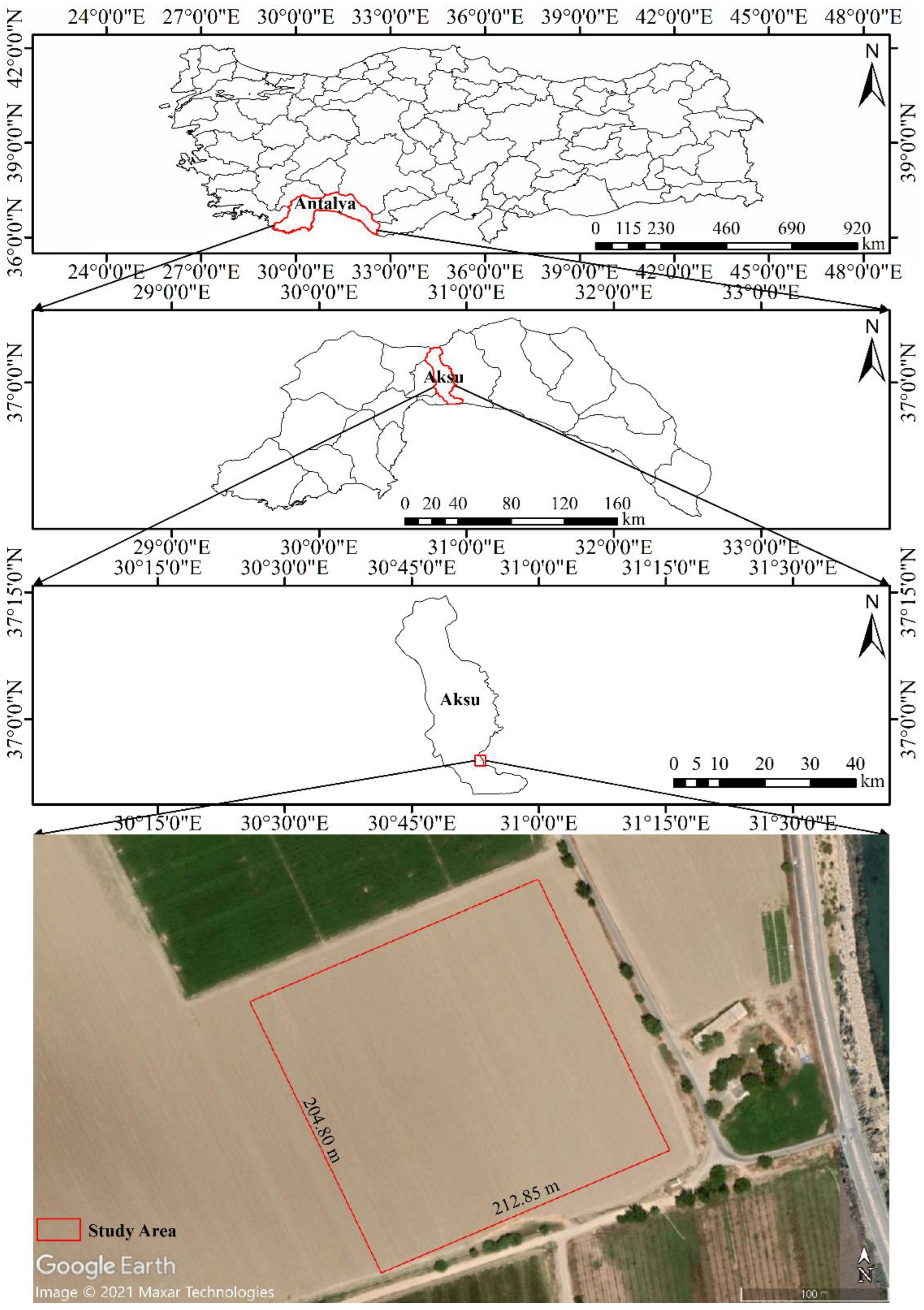
2.1. Study Area

The research was conducted at Akdeniz University’s Faculty of Agriculture’s Aksu Research and Application Farm (30°53′07.06″ N, 36°55′07.92″ E), which is located in the Aksu district of Antalya, Turkey, 20 km from the city center (Figure 1). The study area has been determined to be approximately 43 decares of this farm’s total size of 1100 decares. There are no settlements nor industrial facilities near the study area. The region is covered with agricultural fields and the study area is a research and application farm, where controlled agricultural production is carried out. The study area is relatively flat (having a slope of less than 1%) and has a clay loam soil texture. The region has a Mediterranean climate. In the summer, when maize is planted as a second crop after wheat harvest, the weather is hot and dry.
On 17 July 2019, silage maize seeds were planted as the second crop in the study area after the wheat was harvested. The study area received chiseling on 15 August, inter-row hoeing and fertilization on 20 August, and irrigation operations on 22 August and between 9 and 13 September 2019. Maize was harvested on 31 October 2019, while the plant was still green.

2.2. Satellite Images

In this study, images from the Sentinel-1 SAR and Sentinel-2 optical satellites were used, which are both freely available [48] and have a high spatial and temporal resolution. The Earth Observation Satellites Sentinel-1 and Sentinel-2 were developed as part of the Copernicus Program [49]. Sentinel-1 is made up of two satellites, Sentinel-1A and Sentinel-1B, that share the same orbital plane and characteristics. They have a 180-degree orbital phase difference. Sentinel-1A was launched on 3 April 2014 and Sentinel-1B was launched on 25 April 2016. Sentinel-1, which is equipped with an advanced C-band SAR sensor with a center frequency of 5.405 GHz and thus capable of acquiring images in all weather conditions day and night, acquires images in the ascending and descending orbit directions. At the equator, a single Sentinel-1 satellite in the same orbital direction has a revisit time of 12 days, which is reduced to 6 days when Sentinel-1A and Sentinel-1B satellites are used together [50,51]. Sentinel-2, like Sentinel-1, is made up of two satellites, Sentinel-2A and Sentinel-2B, that share the same orbital plane with an orbital phase difference of 180 degrees and the same characteristics. Sentinel-2A was launched on 23 June 2015, followed by Sentinel-2B on 7 March 2017. At the equator, a single Sentinel-2 satellite carrying an innovative multispectral sensor with 13 spectral bands takes 10 days to revisit, but this time is sliced in half when Sentinel-2A and Sentinel-2B satellites are used together [52,53].

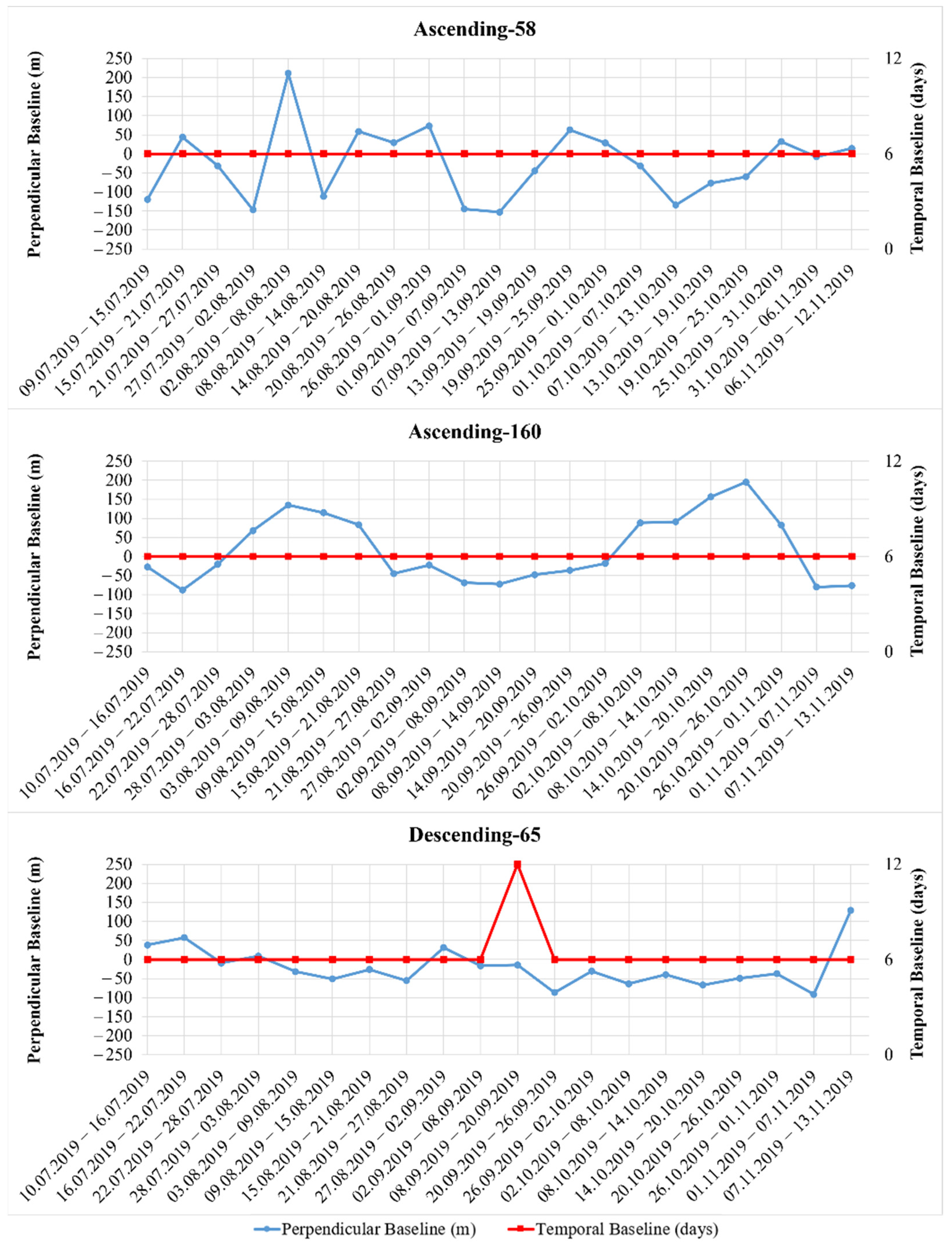
2.2.1. Sentinel-1 SAR Images

All Sentinel-1 (Sentinel-1A and Sentinel-1B) images covering the study area (a total of 65 images) acquired from three different orbits in ascending and descending orbital directions between 9 July and 13 November 2019 were used in the study. For accelerating downloading process, two data hubs, Copernicus Open Access Hub (https://scihub.copernicus.eu/dhus/#/home (accessed on 3 December 2020)) and ASF Data Search Vertex (https://search.asf.alaska.edu/#/ (accessed on 3 December 2020)), which store the same datasets, were used. The images used were Level-1 Single Look Complex (SLC) products with dual polarization (VV and VH), which contain amplitude and phase information and were acquired in the Interferometric Wide Swath (IW) mode, which is the default imaging mode over the land surface. Figure 2 depicts the footprints (coverage areas) of the satellite images used, while Table 1 lists their characteristics and Table 2 lists their acquisition dates.

2.2.2. Sentinel-2 Optical Images

All Sentinel-2 (Sentinel-2A and Sentinel-2B) images (a total of 25 images) covering the study area and acquired between 9 July and 13 November 2019 were used in the study. Sentinel-2 images were downloaded from Copernicus Open Access Hub (https://scihub.copernicus.eu/dhus/#/home (accessed on 17 June 2020)). The images used are Level-2A products, which are orthorectified to the UTM/WGS84 projection, radiometrically, geometrically, and atmospherically corrected, and contain Bottom-of-Atmosphere (BOA) reflection values. Table 3 lists the characteristics of the satellite images used and Table 4 lists their acquisition dates.

2.3. In Situ Data

Plant heights were measured with a 3 m steel tape measure in the field on 11 different dates simultaneously with satellite images. The Magellan eXplorist 610 handheld GPS was used to determine the coordinates of the points where the plant height was measured. Plant height measurements were taken at 20 different points with 10 m intervals on a single row and 16 different points at 50 m intervals in the interior of the study area; 36 different points in total were selected randomly not based on a specific methodology to reflect the general condition of the study area. The average plant height was calculated for each date the plant height measurements were taken. Figure 3 depicts average maize heights measured in the field.

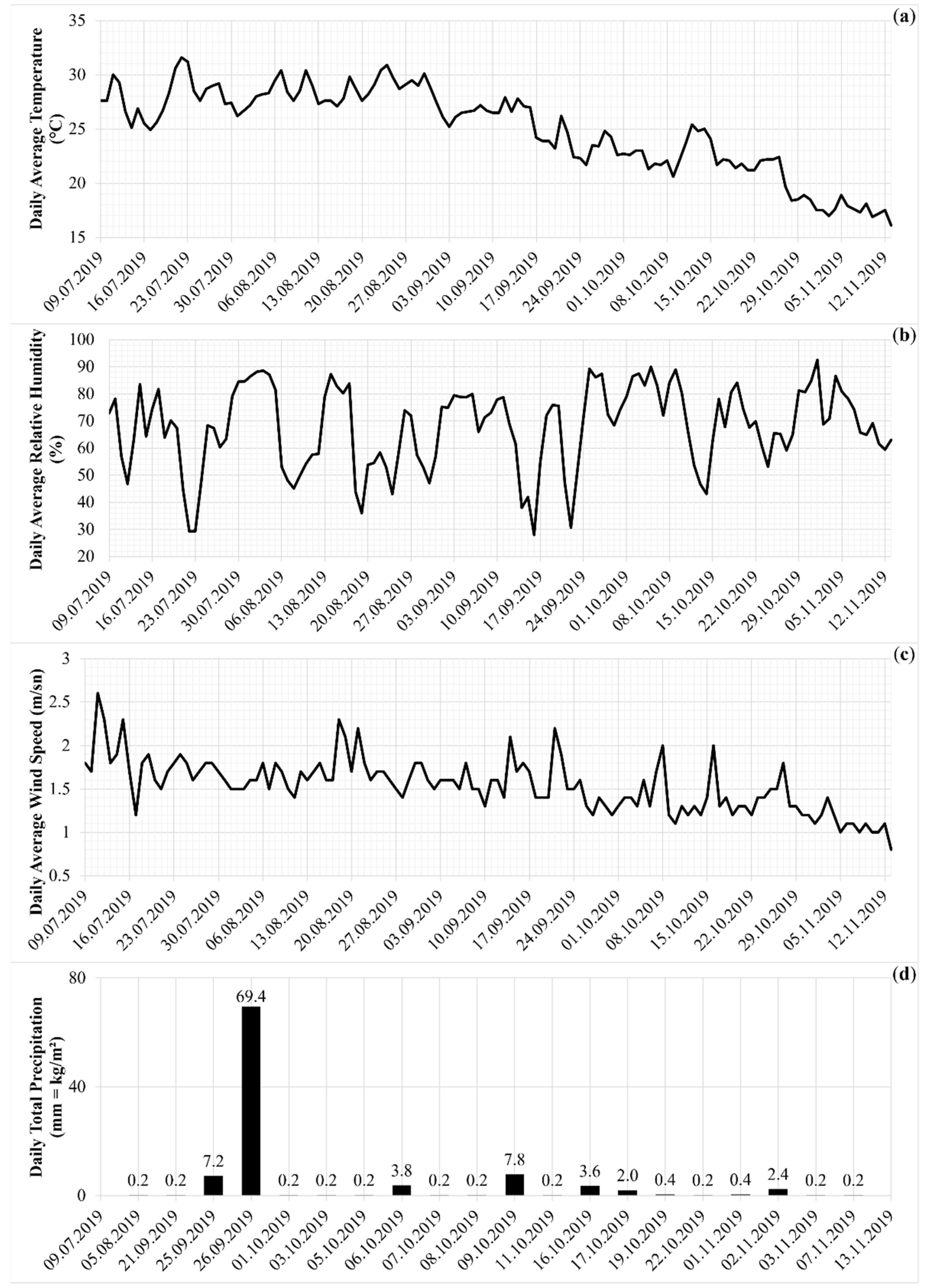
2.4. Meteorological Data

The study used meteorological data from Aksu/Boztepe TİGEM (General Directorate of Agricultural Enterprises) Station 17895, which is the closest observation network to the study area (approximately 2.5 km away from the study area), between 9 July and 13 November 2019, to better evaluate the values obtained from satellite images. Figure 4 depicts the meteorological data used.

2.5. Satellite Images Processing

A Lenovo Legion 5 15IMH05H laptop computer was used for the processing of satellite images. The computer used has an Intel Core i7-10750H CPU 2.60 GHz processor, 16 GB DDR4 RAM, NVIDIA GeForce GTX 1660 Ti 6GB GDDR6 graphics card, and 500 + 500 GB SSD memory.

2.5.1. Sentinel-1 SAR Images Processing

Sentinel-1 images were processed in three different ways in this study, as shown in Figure 5’s flowchart, to calculate backscatter values, interferometric coherence values, and plant heights. Sentinel-1 images were processed using the Sentinel Application Platform (SNAP) software’s Sentinel-1 Toolbox (version 8.0.4). SNAP is an open-source software for the exploitation of Earth Observation satellite images [56] and it is available to download from the Science Toolbox Exploitation Platform (STEP) (https://step.esa.int/main/download/snap-download/ (accessed on 31 July 2021)). To accelerate the process, the SNAP software’s Graph Builder and Batch Processing tools were used.
To calculate backscatter values, the images were processed applying these steps: (1) split; (2) apply orbit file; (3) thermal noise removal; (4) radiometric calibration; (5) deburst; (6) multilooking (the number of looks applied to images acquired from Ascending-58 and Descending-65 orbits was four × one, and to images acquired from Ascending-160 orbit was three × one); (7) Range-Doppler Terrain Correction [57,58] (Shuttle Radar Topography Mission (SRTM) 1 arc-second Height (1Sec HGT) Digital Elevation Model (DEM) data with a spatial resolution of 30 m were used and the images were orthorectified to the UTM/WGS84 projection and the pixel spacings of the final products were 13.96 m); (8) subset; (9) converting backscatter values from linear scale to logarithmic scale (σ0dB = 10 × log10 σ0); (10) calculating VH/VV ratio in dB (σ0VH/VV = σ0VH − σ0VV) [59]; and (11) extraction of median backscatter (σ0VV, σ0VH, and σ0VH/VV) values for the study area.
Because temporal decorrelation is one of the most important sources of decorrelation in areas covered with vegetation [60,61], interferometric coherence values were calculated using consecutively acquired Sentinel-1 image pairs to avoid temporal decorrelation. Figure 6 depicts the interferometric properties of satellite image pairs used in the study.
To calculate interferometric coherence values, the images were processed applying these steps: (1) split (in this processing step, the VV and VH polarizations were chosen separately to apply the InSAR technique and the following steps were performed separately for both polarizations); (2) apply orbit file; (3) coregistration of image pairs (SRTM 1 Sec HGT DEM data were used); (4) calculating coherence values; (5) deburst; (6) multilooking; (7) Range-Doppler Terrain Correction (SRTM 1 Sec HGT DEM data were used and the images were orthorectified to the UTM/WGS84 projection and the pixel spacings of the final products were 13.96 m); and (8) extraction of median interferometric coherence (γVV and γVH) values for the study area.
The perpendicular baseline between satellite image pairs affects sensitivity to topography [62]. Height of ambiguity (HoA) (height information for 1 phase cycle) decreases as the perpendicular baseline increases [63] and smaller HoA more precisely describes the topographic features of the terrain [64]. As a result, smaller HoA and larger perpendicular baselines provide greater precision when calculating plant heights [2,65]. However, as shown in Figure 6, the perpendicular baseline between consecutive Sentinel-1 image pairs was very small. The smaller the perpendicular baseline the less accurate the topography estimate is [66]. Nonetheless, two Sentinel-1 image pairs (shown in Table 5) were selected to calculate plant heights in this study. Among the image pairs used in the study, these had the largest perpendicular baseline and the lowest HoA.
To calculate plant heights, the images were processed applying these steps: (1) split (in this processing step, the VV polarization with higher interferometric coherence values was chosen); (2) apply orbit file; (3) coregistration of image pairs (SRTM 1 Sec HGT DEM data were used); (4) interferogram formation (by subtracting flat-earth phase); (5) deburst; (6) multilooking (in this processing step, phase and intensity bands were not selected to avoid errors while performing this process in the SNAP software; intensity and phase bands were produced from complex I and Q bands after performing the multilook); (7) Goldstein Phase Filtering [67]; (8) subset; (9) phase unwrapping with SNAPHU Unwrapping plug-in (version 2.0.4) in SNAP software (while the phase image was exported to SNAPHU, TOPO for Statistical-cost mode, MCF for Initial method, 1 for Number of Tile Rows and Number of Tile Columns was selected) [68]; (10) DEM generation; (11) Range-Doppler Terrain Correction (SRTM 1 Sec HGT DEM data were used, the images were orthorectified to the UTM/WGS84 projection, and the pixel spacings of the final products were 13.96 m); (12) DEMs were stacked in the same file (the DEM generated from the first image pair (2 and 8 August) represents the stage where the average plant heights are 0.33 m and this DEM is assumed as Digital Terrain Model (DTM). The DEM generated from the second image pair (20 and 26 October) represents the stage where the average plant heights are 2.80 m and this DEM is assumed as Digital Surface Model (DSM) (Table 5)); and (13) calculation of plant heights for the study area by subtracting the DTM from the DSM [2].

2.5.2. Sentinel-2 Optical Image Processing

Sentinel-2 images were processed as shown in the flowchart in Figure 7 to calculate NDVI and other biophysical variables (LAI, fCover, and CW) values. Sentinel-2 images were processed using the SNAP software’s Sentinel-2 Toolbox (version 8.0.4) (https://step.esa.int/main/download/snap-download/ (accessed on 31 July 2021)). To accelerate the process, the SNAP software’s Graph Builder and Batch Processing tools were used.
To calculate NDVI and other biophysical variables (LAI, fCover, and CW) values, the images were processed by applying these steps: (1) all bands resampled to 10 m; (2) subset; (3) calculation of NDVI, LAI, fCover, and CW values (NDVI values were calculated using Equation (1) [69], while LAI, fCover, and CW values were calculated using Biophysical Processor in the SNAP software. NDVI, LAI, and fCover images had a resolution of 10 m and CW images had a resolution of 20 m); and (4) extraction of median NDVI, LAI, fCover, and CW values for the study area.
NDVI   = NIR RED NIR + RED

3. Results and Discussion

3.1. Sensitivity of Backscatter Values to Maize Growth

Some studies have reported that polarization ratios were shown to be less responsive to changes in soil moisture [13,23,70,71], less affected by precipitation events [59], and more sensitive to maize growth [71,72,73]. Therefore, in addition to σ0VV and σ0VH values, σ0VH/VV values were also investigated in this study. Figure 8 depicts the median backscatter values (σ0VV, σ0VH, and σ0VH/VV) of Sentinel-1 satellite images acquired from three different orbits for the study area.
Prior to planting, the backscatter values of images acquired from three different orbits were low. After planting, a decrease was observed in σ0VV and σ0VH values of images acquired from three different orbits on 21 and 22 July, although the radar’s look direction is nearly perpendicular to the row direction in images acquired from Ascending-58 and Ascending-160 orbits (see Figure 2) and even though backscatter values are expected to increase due to increasing soil roughness [39,74,75]. The sparse soil after planting may have contributed to the deeper penetration of radar signals and this decrease in backscatter values. Similar decreases were observed in some studies [10,13]. On the other hand, the σ0VH value of the image acquired from the Ascending-160 orbit on 22 July remained nearly constant. This can be explained by the fact that lower incidence angles are less sensitive to surface roughness [76] and the cross-polarization is less affected by the row direction [9,23]. The findings of this study contradict those of Formaggio et al. [22] and Mascolo et al. [77].
After being low for a while, the backscatter values of images acquired from three different orbits began to respond to maize growth, and backscatter values increased as maize grew [10,19,30,31,42,72,78,79,80,81], as expected for broadleaf crops [27,82,83]. The backscatter values of images acquired from the Ascending-58 orbit with a larger incidence angle gave the earliest response to maize growth as of 2 August (after the average maize height exceeded 25 cm). Therefore, it was discovered that images acquired with large incidence angles can be effective in monitoring the early growth stages of maize. Contrary to McNairn et al. [29,34], the backscatter values of images acquired from three different orbits continued to increase until 19 September (until the average maize height exceeded 250 cm [13]), at which point they reached saturation [10,32,59,70,77,84,85,86,87], which is a well-known effect for crops with higher biomass [8,42]. Before harvest, a slight decrease was observed in σ0VV and σ0VH values of images acquired from three different orbits on 14, 25, and 26 October (when the average maize height was 275–280 cm). The decreases in backscatter values could indicate that the canopy water content has begun to decline and that it is time to harvest the silage maize.
The backscatter values of images acquired from three different orbits differed after harvest. In general, the backscatter values of the first images acquired after harvest either remained nearly constant or decreased slightly and the backscatter values of the second images acquired after harvest either continued to decrease gradually or decreased sharply. This is most likely due to the green residues that remained in the field and dried out gradually after harvest [13]. Previous studies have also found that backscatter values decrease after maize harvesting [10,13,32,40,70,81,84].
On the other hand, a clear trend was not observed in σ0VH/VV values of images acquired from three different orbits. The σ0VH/VV values of images acquired from the Ascending-58 orbit with a larger incidence angle gave the best response to maize growth. The σ0VH/VV values of images acquired from this orbit increased from 2 August (after the average maize height exceeded 25 cm) to 19 September (until the average maize height exceeded 250 cm) and then reached saturation, similar to σ0VV and σ0VH values of images acquired from this orbit. Before harvest, an increase in σ0VH/VV value was observed due to a slight decrease in σ0VV on 25 October (when the average maize height was 280 cm). This increase may be due to the decrease in canopy water content before harvest [40]. The σ0VH/VV value of the first image acquired from this orbit after harvest showed a slight decrease and the σ0VH/VV value of the second image acquired from this orbit after harvest showed a sharp decrease. However, the σ0VH/VV values of images acquired from the Ascending-160 orbit did not give a significant response to maize growth. This indicates that using the σ0VH/VV values of images acquired with lower incidence angles is not useful for monitoring maize growth. Furthermore, it is quite difficult to determine the date of harvest using the σ0VH/VV values of images acquired from the Descending-65 orbit [59].

3.1.1. The Effects of Irrigation, Chiseling, and Inter-Row Hoeing Operations on Backscatter Values

Irrigation operations in the study area were carried out using the furrow irrigation method (also known as the flood or surface irrigation method). Each irrigation operation lasted 10 h. Since there is no possibility of splashing water on the plant leaves as a result of the irrigation operation with this method, the effect of the water droplets remaining on the plant leaves after the irrigation operations on the backscatter values was not evaluated.
After irrigations, it is an expected situation that the dielectric constant of the soil increases due to the increased soil moisture and thus the backscatter values increase [39,75]. After irrigation on 22 August, an increase was observed in σ0VV and σ0VH values of images acquired from three different orbits on 26 and 27 August (when the average maize height was 104–105 cm) due to increased soil moisture. In addition, the σ0VV and σ0VH values of images acquired from Ascending-160 and Descending-65 orbits on 2 September (when the average maize height was 128 cm) were also high due to the soil still being moist. This is most likely due to greater penetration of the radar signals into the maize canopy at a lower incidence angle.
After irrigations between 9 and 13 September, an increase was also observed in σ0VV and σ0VH values of images acquired from Ascending-58 and Ascending-160 orbits on 13 and 14 September (when the average maize height was 233–237 cm). This indicates that the effect of soil moisture on radar signal should not be ignored even for well-developed crops [88] since there was no precipitation event in this date range. It was also observed by other researchers that backscatter values were sensitive to soil moisture when the maize canopy was at the highest biomass [89,90] even at large incidence angles [90]. The sensitivity of backscatter values to soil moisture is due to scattering along the soil–vegetation pathway, which also includes contributions from soil moisture [89,90] due to the 70 cm large row spacing of maize [40,91]. The results obtained from this study disprove Sun et al. [92], who reported that C-band cannot penetrate soil through vegetation and that data obtained from the Sentinel-1 SAR satellite are sensitive to vegetation. On the other hand, due to the absence of an image acquired from the Descending-65 orbit on 14 September, the effect of irrigation between 9 and 13 September could not be clearly observed in the backscatter values of images acquired from this orbit.
Contrary to Paloscia [93], it was observed that increased soil roughness under sparse vegetation after chiseling and inter-row hoeing did not have much effect on the backscatter values of images acquired from three different orbits on 15 August (when the average maize height was 61 cm), 20 August (when the average maize height was 73 cm), and 21 August (when the average maize height was 78 cm). In addition, it was observed that the σ0VH/VV values of images acquired from Ascending-58 and Descending-65 orbits (particularly Descending-65 orbit) were not affected much by soil roughness after planting, chiseling, and inter-row hoeing, and increased soil moisture after irrigation [13,23,70,71].

3.1.2. The Effect of Precipitation on Backscatter Values

Although clouds have little or no effect on SAR signals depending on the wavelength used, precipitation [94,95] and water droplets on the canopy [95,96] have a significant impact on SAR backscatter.
After precipitation events of 7.2 mm on 25 September and 69.4 mm on 26 September, an increase was observed in σ0VV and σ0VH values of images acquired from three different orbits on 25 and 26 September (when the average maize height was 257–258 cm), contrary to Selvaraj et al. [97]. Other studies have also reported that the backscatter values increase after precipitation [59,70,96]. In addition, some of the backscatter values of images acquired from three different orbits on 1, 2, and 8 October (when the average maize height was 264–271 cm) were also high. This is most likely due to water droplets that remained on the plant leaves after light precipitations or because the radar signals penetrated the maize canopy and became sensitive to soil moisture. The latter is more likely, as images from the Ascending-160 orbit were more sensitive to precipitation events. A similar finding was found by El Hajj et al. [89].
In addition, an increase was observed in σ0VV and σ0VH values of the image acquired from the Descending-65 orbit on 20 October (when the average maize height was 280 cm). Given that water droplets on the canopy affect backscatter values [95,96] and that water droplets on the canopy increase backscatter values [74], this increase in backscatter values of images acquired at 06:59 a.m. local time (UTC+03:00) from Descending-65 orbit is most likely due to water droplets on plant leaves due to early morning dew.
Furthermore, an increase was observed in σ0VV values of images acquired from the Ascending-160 orbit after harvest on 1 November. Given that the radar’s look direction in images acquired from this orbit is nearly perpendicular to the row direction, this is most likely due to double-bounce scattering between maize residues and the soil surface [98] after the precipitation event. On the other hand, it was observed that the σ0VH/VV values of images acquired from Ascending-58 and Descending-65 orbits were not affected much by precipitation [59].

3.2. Sensitivity of Interferometric Coherence Values to Maize Growth

Figure 9 depicts the median interferometric coherence values (γVV and γVH) of Sentinel-1 satellite image pairs acquired from three different orbits for the study area.
The interferometric coherence values of image pairs acquired from Ascending-58 and Descending-65 orbits with larger incidence angles were largely similar to each other. Prior to planting, the γVV values of image pairs acquired from both orbits were high [10], as expected, since there is no temporal decorrelation in bare soils [61]. The planting operation between the two consecutive images caused the γVV values of these image pairs to drop sharply because of the change in soil roughness [99]. Therefore, a sudden decrease observed in interferometric coherence values may be an indication of the beginning of agricultural activity in bare soils [46].
On the other hand, the interferometric coherence values of image pairs acquired from the Ascending-160 orbit with a lower incidence angle were found to be quite different. The interferometric coherence values of image pairs acquired from this orbit were found to be quite low, particularly before the planting.
The γVV values of the next image pairs acquired from three different orbits after planting were high [10,99] as there was no significant plant growth during this time. The γVV values started to decrease as the maize grew [10,46,99,100], since the plants develop dynamically during the time period when image pairs are acquired [61]. The γVV values of image pairs acquired from Ascending-58 and Descending-65 orbits reached the lowest levels after the average maize height exceeded 60 cm and remained low throughout the growing season until harvest [10,43]. On the other hand, the γVH values of image pairs acquired from these orbits remained low throughout the entire growing season [10].
The γVV values of image pairs acquired from three different orbits differed after harvest. In general, the γVV values of the second image pairs acquired after harvest were quite high. This is most likely the result of the green residues left in the field after harvest completely dried out. Similar findings have been reported by Amherdt et al. [43]. Other researchers also noticed that the interferometric coherence values were high after harvest [10,70,100,101], which is a useful indicator for harvesting [70].

3.2.1. The Effects of Irrigation, Chiseling, and Inter-Row Hoeing Operations on Interferometric Coherence Values

It was observed that increased soil roughness under sparse vegetation after chiseling and inter-row hoeing, and increased soil moisture after irrigations did not have much effect on the interferometric coherence values of image pairs acquired from Ascending-58 and Descending-65 orbits with larger incidence angles. Blaes and Defourny [99] also found that interferometric coherence values were less sensitive to soil moisture than backscattering coefficients.
On the other hand, the sharp decrease in the γVV value of the image pair acquired on 9 and 15 August from the Ascending-160 orbit with a lower incidence angle could be due to increased soil roughness after chiseling just before the image acquisition on 15 August. Furthermore, the high γVV value of the image pair acquired from this orbit, particularly on 27 August and 2 September, may be due to increased soil moisture after irrigation on 22 August. Similarly, the irrigation between 9 and 13 September may have caused a high γVV value of the image pair acquired from this orbit on 14 and 20 September. This indicates that the interferometric coherence values of image pairs acquired with lower incidence angles may be sensitive to increased soil roughness in sparse vegetation and increased soil moisture even in dense vegetation.

3.2.2. The Effect of Precipitation on Interferometric Coherence Values

Some increases were observed in γVV and γVH values of image pairs acquired from Ascending-58 and Descending-65 orbits. These increases, observed when the average maize height was in the range of 260 to 275 cm, were likely due to precipitation events [10]. Furthermore, it was discovered that precipitation events had a greater impact on the interferometric coherence values of image pairs acquired from the Ascending-160 orbit with lower incidence angles. The fact that both γVV and γVH values of image pairs acquired from this orbit were so high, particularly after the 69.4 mm heavy precipitation event on 26 September, suggests that the plant geometry may have changed because of the heavy precipitation [102] and, as a result, scattering from moist soil may have dominated the backscattered signal by penetrating the maize canopy of radar signals. Considering that γVH values, which are low throughout the growing season, were higher after precipitation events, it was discovered that high γVH values can provide information about regional precipitation. The findings of this study contradict the findings of Santoro et al. [103], who reported that precipitation decreased interferometric coherence values.

3.3. Sensitivity of NDVI and Other Biophysical Variables (LAI, fCover, and CW) to Maize Growth

NDVI is one of the most widely used vegetation indices [15,18]. The main reason for using NDVI values in this study is that these values have been investigated many times before to monitor crop growth; interpretation of these values is quite well. On the other hand, backscatter values were compared with NDVI [13,23,32], LAI [36], and fCover (or FVC) [38,104] values in some previous studies. In addition to NDVI, LAI, and fCover values, CW values are also included in this study since SAR data are known to be highly sensitive to changes in canopy water content. All these values were compared with plant heights in this study since no local samples were collected regarding these values.
Cloud cover, fog, and smoke hinder passive optical sensors from getting information about the earth’s surface [24], therefore values derived from images acquired on dates when cloud cover and/or fog were present over the study area and specified in Table 4 were not evaluated. Figure 10 depicts the median NDVI, LAI, fCover, and CW values derived from Sentinel-2 satellite images.
NDVI, LAI, fCover, and CW values that were very low before planting also remained very low for a long time after planting [85]. After being low for a while, NDVI, LAI, fCover, and CW values began to respond to maize growth and these values increased as the maize grew. NDVI gave the earliest response to maize growth as of 10 August (after the average maize height exceeded 50 cm). NDVI, LAI, fCover, and CW values continued to increase until 29 September (until the average maize height exceeded 260 cm), at which point they reached saturation, which is a well-known effect for densely vegetated areas. Similar findings have been reported in previous studies for NDVI [13,15,16,17,23,26,32,84,105,106,107,108] and LAI [17,19,85] values.
Before harvest, NDVI, LAI, fCover, and CW values all dropped slightly, particularly on 29 October (when the average maize height was 280 cm). These decreases in NDVI, LAI, fCover, and CW values could indicate that the canopy water content has begun to decline and that it is time to harvest the silage maize. After harvest, NDVI, LAI, fCover, and CW values all decreased sharply [13,16,107].
It was observed that increased soil roughness after planting and under sparse vegetation after chiseling and inter-row hoeing and increased soil moisture after irrigations did not affect NDVI, LAI, fCover, and CW values. Ameline et al. [84] also reported that changes in soil moisture did not affect NDVI values.
On the other hand, some differences were observed in NDVI, LAI, fCover, and CW values, which did not reflect the true trend (e.g., the difference on 4 September for all values). There was cloud cover and/or fog near the study area on the dates when these differences were observed. Therefore, it was determined that cloud cover and/or fog near the study area, even if they were not directly above the study area, influenced these values. Cloud cover and/or fog near the study area had the least impact on NDVI, while cloud cover and/or fog had the most impact on CW.

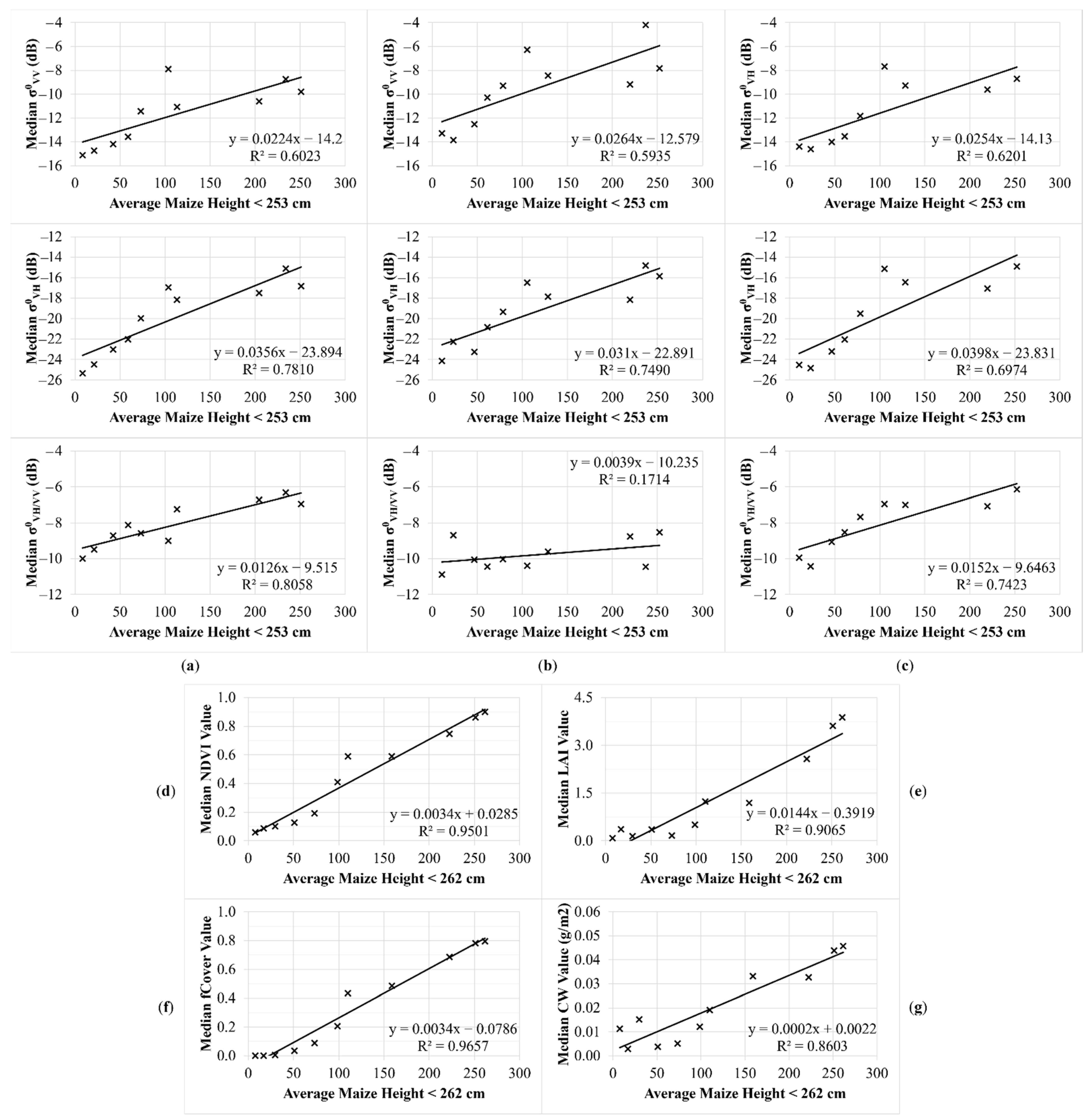
3.4. Sensitivity Analysis of Backscatter, NDVI, LAI, fCover, and CW Values to Maize Height

Figure 11 depicts the coefficient of determination (R2) between Sentinel-derived values (backscatter, NDVI, LAI, fCover, and CW) and measured maize height.
Contrary to other studies [29,33,34,38,104], backscatter values derived from Sentinel-1 images were sensitive to changes in crop growth until the average maize height exceeded 250 cm, while NDVI, LAI, fCover, and CW values derived from Sentinel-2 images were sensitive to changes in crop growth until the average maize height exceeded 260 cm. Since backscatter values reached saturation after maize height exceeded 253 cm and Sentinel-2-derived values reached saturation after maize height exceeded 262 cm, these values then remained insensitive to minor changes in maize height.
Among the backscatter values derived from Sentinel-1, the σ0VH/VV values of images acquired from the Ascending-58 orbit with the largest incidence angle showed the best correlation with maize height (R2 = 0.81), while the σ0VH/VV values of images acquired from the Ascending-160 orbit with the lowest incidence angle showed the worst (R2 = 0.17). Among the values derived from Sentinel-2, fCover values showed the best correlation with maize height (R2 = 0.97), while CW values showed the worst (R2 = 0.86). Furthermore, it was determined that the values derived from Sentinel-2 were more sensitive to maize height. This is most likely due to Sentinel-1-derived backscatter values being sensitive to soil moisture and precipitation events.

3.5. Maize Heights Calculated Using Sentinel-1 Satellite Images

Figure 12 depicts the DEMs generated using Sentinel-1 satellite image pairs for the study area and Figure 13 depicts the maize heights calculated by subtracting DTM from DSM. As previously stated in Section 2.5.1, the average maize height was 0.33 m in the date range when the first image pair was acquired (2 and 8 September) and 2.80 m in the date range when the second image pair was acquired (20 and 26 October). In other words, maize heights grew by an average of 2.47 m between the dates when Sentinel-1 image pairs used to calculate plant heights were gathered. The average plant height calculated using Sentinel-1 images, on the other hand, was 2.95 m (Table 6). This analysis finds that by using Sentinel-1 image pairs acquired in monostatic repeat-pass mode the average maize height was calculated with an inaccuracy of roughly 50 cm. However, Figure 12 and Figure 13 indicate that the height value range is very wide and that the height values fluctuate greatly from pixel to pixel. Table 6 shows those plant heights calculated using Sentinel-1 image pairs range between −3.20 m and +8.35 m, with a large standard deviation. This is most likely due to erroneous phase unwrapping caused by some pixels’ poor interferometric coherence values. As a result, it was discovered that the average plant height value obtained using Sentinel-1 images was near to the real plant height value by coincidence. Sentinel-1 image pairs with large perpendicular baseline are difficult to find [64] and thus Sentinel-1 images are not suitable enough for DEM generation [66], therefore using satellite image pairs with larger perpendicular baseline acquired in bistatic single-pass mode can help to obtain more precise plant heights.

4. Conclusions

In this study, SAR and optical satellite images were used to monitor silage maize throughout the entire growing season and plant heights were calculated using Sentinel-1 image pairs acquired in monostatic repeat-pass mode. The study was conducted on a field scale in Turkey between 9 July and 13 November 2019. The sensitivity of Sentinel-derived values to maize growth, tillage practices (planting, harvest, irrigation, etc.,), precipitation events, and maize height was investigated.
This study demonstrated that combining SAR and optical satellite images can give crucial information for monitoring maize growth. The main conclusions are summarized as follows:
(1)
Before planting, backscatter and Sentinel-2-derived values were low, while interferometric coherence values were generally high. After planting, σ0VV, σ0VH, and γVV values of images acquired, especially with larger incidence angles, responded to planting operations. While NDVI, LAI, fCover, and CW values are low, the decreases observed in backscatter and interferometric coherence values can be used as an indicator of the beginning of agricultural activity in the maize fields.
(2)
Among all Sentinel-derived values, the earliest response to maize growth was given by backscatter values of images acquired from Ascending-58 orbit with a larger incidence angle after average maize height exceeded 25 cm. As the σ0VV, σ0VH, and σ0VH/VV values increased, the γVV values decreased. Therefore, SAR data acquired at larger incidence angles can be used to identify and monitor the early growth stages of maize.
(3)
Backscatter values increased after irrigation operations. Therefore, observed increases in backscatter values can be used to monitor irrigation operations. In addition, backscatter values were sensitive to irrigation operations even when the average maize height was about 235 cm. This demonstrated that Sentinel-1’s C-band sensor was able to penetrate dense vegetation. Therefore, it should not be ignored that the radar signals may become sensitive to soil moisture, especially in maize fields with wide row spacing.
(4)
Backscatter and interferometric coherence values of images acquired with lower incidence angles were more affected by precipitation events. γVH values, which were low throughout the growing season, became significantly higher after precipitation events. Therefore, high values of γVH can provide information about regional precipitation.
(5)
Among all Sentinel-derived values, fCover derived from Sentinel-2 was the most sensitive to maize height (R2 = 0.97). The value derived from Sentinel-1 that is the most sensitive to maize height was the σ0VH/VV value of images acquired from the Ascending-58 orbit with larger incidence angles (R2 = 0.81). Using these values in combination with the γVV values of image pairs acquired with large incidence angles (as they are less affected by irrigation operations and precipitation events) can provide more reliable information for monitoring maize growth.
(6)
A slight decrease in backscatter, NDVI, LAI, fCover, and CW values was observed before harvest. These decreases can be considered as an indication that the canopy water content of silage maize has started to decrease and it is time to harvest. In addition, these decreases can also be considered as an indication that the grain maize has passed through the final growth stages. In addition, since backscatter and interferometric coherence values were sensitive to crop residues left in the field after harvest and precipitation can make it difficult to determine the harvest date, values derived from Sentinel-2 that show a drastic decline after harvest can help determine the harvest date more precisely.
(7)
On the other hand, calculation of plant heights may be an alternative to overcome the saturation effects observed in values derived from SAR and optical images. In this study, using Sentinel-1 image pairs acquired in monostatic repeat-pass mode, plant heights were calculated with an error of about 50 cm. However, it was determined that these values were close to the actual plant height value by coincidence. In future studies, plant heights can be calculated more precisely using image pairs acquired in bistatic single-pass mode with a larger perpendicular baseline and a lower HoA.

Author Contributions

Conceptualization, M.T., İ.A. and N.D.; methodology, M.T., İ.A. and N.D.; software, İ.A. and N.D.; validation, İ.A. and M.T.; formal analysis, İ.A.; investigation, İ.A.; resources, M.T.; data curation, İ.A. and M.T.; writing—original draft preparation, İ.A.; writing—review and editing, İ.A. and N.D.; visualization, İ.A.; supervision, M.T. and N.D. All authors have read and agreed to the published version of the manuscript.

Funding

This research received no external funding.

Institutional Review Board Statement

Not applicable.

Data Availability Statement

Available upon request.

Acknowledgments

Authors acknowledge Burcin Donmez for language editing, Sami Canbolat from Faculty of Agriculture, Research and Application Farm for supporting field work, and Meteorological Department of Antalya for providing the weather datasets. We appreciate anonymous reviewers for their constructive comments to help us to improve the paper.

Conflicts of Interest

The authors declare no conflict of interest.

References

  1. Serna-Saldivar, S.O. Preface. In Corn: Chemistry and Technology, 3rd ed.; Serna-Saldivar, S.O., Ed.; Woodhead Publishing: Duxford, UK; AACC International Press: Washington, DC, USA, 2019; pp. xv–xvi. ISBN 9780128118863. [Google Scholar]
  2. Hütt, C.; Tilly, N.; Schiedung, H.; Bareth, G. Potential of multitemporal TanDEM-X derived crop surface models for maize growth monitoring. Int. Arch. Photogramm. Remote Sens. Spat. Inf. Sci. 2016, XLI-B7, 803–808. [Google Scholar] [CrossRef] [Green Version]
  3. Tian, F.; Wu, B.; Zeng, H.; Zhang, X.; Xu, J. Efficient identification of corn cultivation area with multitemporal synthetic aperture radar and optical images in the Google Earth Engine Cloud Platform. Remote Sens. 2019, 11, 629. [Google Scholar] [CrossRef] [Green Version]
  4. Su, W.; Sun, Z.; Chen, W.-h; Zhang, X.; Yao, C.; Wu, J.; Huang, J.; Zhu, D. Joint retrieval of growing season corn canopy LAI and leaf chlorophyll content by fusing Sentinel-2 and MODIS images. Remote Sens. 2019, 11, 2409. [Google Scholar] [CrossRef] [Green Version]
  5. Serna-Saldivar, S.O.; Perez Carrillo, E. Food uses of whole corn and dry-milled fractions. In Corn: Chemistry and Technology, 3rd ed.; Serna-Saldivar, S.O., Ed.; Woodhead Publishing: Duxford, UK; AACC International Press: Washington, DC, USA, 2019; pp. 435–467. ISBN 9780128118863. [Google Scholar]
  6. Martinez, E.L.; Fernandez, F.J.B. Economics of production, marketing and utilization. In Corn: Chemistry and Technology, 3rd ed.; Serna-Saldivar, S.O., Ed.; Woodhead Publishing: Duxford, UK; AACC International Press: Washington, DC, USA, 2019; pp. 87–107. ISBN 9780128118863. [Google Scholar]
  7. Turkish Statistical Institute (TURKSTAT). Bitkisel Ürün Denge Tabloları, 2020–2021. Available online: https://data.tuik.gov.tr/Bulten/Index?p=Bitkisel-Urun-Denge-Tablolari-2020-2021-45505 (accessed on 12 April 2022).
  8. Soria-Ruiz, J.; Fernandez-Ordonez, Y.; McNairm, H.; Bugden-Storie, J. Corn Monitoring and Crop Yield Using Optical and RADARSAT-2 Images. In Proceedings of the 2007 IEEE International Geoscience and Remote Sensing Symposium (IGARSS), Barcelona, Spain, 23–28 July 2007; pp. 3655–3658. [Google Scholar]
  9. McNairn, H.; Brisco, B. The application of C-band polarimetric SAR for agriculture: A review. Can. J. Remote Sens. 2004, 30, 525–542. [Google Scholar] [CrossRef]
  10. Nasirzadehdizaji, R.; Cakir, Z.; Balik Sanli, F.; Abdikan, S.; Pepe, A.; Calò, F. Sentinel-1 interferometric coherence and backscattering analysis for crop monitoring. Comput. Electron. Agric. 2021, 185, 106118. [Google Scholar] [CrossRef]
  11. Meroni, M.; d’Andrimont, R.; Vrieling, A.; Fasbender, D.; Lemoine, G.; Rembold, F.; Seguini, L.; Verhegghen, A. Comparing land surface phenology of major European crops as derived from SAR and multispectral data of Sentinel-1 and -2. Remote Sens. Environ. 2021, 253, 112232. [Google Scholar] [CrossRef]
  12. Alvino, F.C.G.; Aleman, C.C.; Filgueiras, R.; Althoff, D.; da Cunha, F.F. Vegetation indices for irrigated corn monitoring. Eng. Agric. 2020, 40, 322–333. [Google Scholar] [CrossRef]
  13. Veloso, A.; Mermoz, S.; Bouvet, A.; Le Toan, T.; Planells, M.; Dejoux, J.-F.; Ceschia, E. Understanding the temporal behavior of crops using Sentinel-1 and Sentinel-2-like data for agricultural applications. Remote Sens. Environ. 2017, 199, 415–426. [Google Scholar] [CrossRef]
  14. Liu, C.-a.; Chen, Z.-x.; Shao, Y.; Chen, J.-s.; Hasi, T.; Pan, H.-z. Research advances of SAR remote sensing for agriculture applications: A review. J. Integr. Agric. 2019, 18, 506–525. [Google Scholar] [CrossRef] [Green Version]
  15. Nandibewoor, A.; Hebbal, S.B.; Hegadi, R. Remote monitoring of maize crop through satellite multispectral imagery. Procedia Comput. Sci. 2015, 45, 344–353. [Google Scholar] [CrossRef] [Green Version]
  16. Tunca, E. Evaluation of Using Vegetation Indices and Evapotranspiration Data Obtained from Satellite Data for Yield Estimation of Silage Corn. Master’s Thesis, Ondokuz Mayıs University, Samsun, Turkey, 7 August 2015. [Google Scholar]
  17. Zhang, F.; Zhou, G.; Nilsson, C. Remote estimation of the fraction of absorbed imagesynthetically active radiation for a maize canopy in Northeast China. J. Plant Ecol. 2015, 8, 429–435. [Google Scholar] [CrossRef] [Green Version]
  18. Bhandari, A.K.; Kumar, A.; Singh, G.K. Feature extraction using Normalized Difference Vegetation Index (NDVI): A case study of Jabalpur City. Procedia Technol. 2012, 6, 612–621. [Google Scholar] [CrossRef] [Green Version]
  19. Bahrami, H.; Homayouni, S.; Safari, A.; Mirzaei, S.; Mahdianpari, M.; Reisi-Gahrouei, O. Deep learning-based estimation of crop biophysical parameters using multi-source and multi-temporal remote sensing observations. Agronomy 2021, 11, 1363. [Google Scholar] [CrossRef]
  20. Chaves, M.E.D.; Picoli, M.C.A.; Sanches, I.D. Recent applications of Landsat 8/OLI and Sentinel-2/MSI for land use and land cover mapping: A systematic review. Remote Sens. 2020, 12, 3062. [Google Scholar] [CrossRef]
  21. Chaves, M.E.D.; Soares, A.R.; Sanches, I.D.; Fronza, J.G. CBERS data cubes for land use and land cover mapping in the Brazilian Cerrado agricultural belt. Int. J. Remote Sens. 2021, 42, 8398–8432. [Google Scholar] [CrossRef]
  22. Formaggio, A.R.; Epiphanio, J.C.N.; dos Santos Simões, M. Radarsat backscattering from an agricultural scene. Pesqui. Agropecu. Bras. 2001, 36, 823–830. [Google Scholar] [CrossRef] [Green Version]
  23. Holtgrave, A.-K.; Röder, N.; Ackermann, A.; Erasmi, S.; Kleinschmit, B. Comparing Sentinel-1 and -2 data and indices for agricultural land use monitoring. Remote Sens. 2020, 12, 2919. [Google Scholar] [CrossRef]
  24. Brosinsky, A.; Kuester, T.; Foerster, S.; Kaufmann, H.; Segl, K.; Guanter, L. Principles of Imaging Spectroscopy: Electromagnetic Radiation and Its Interactions with Earth Surface Materials. Available online: https://eo-college.org/resource/principles-of-imaging-spectroscopy/ (accessed on 17 April 2021).
  25. King, M.D.; Platnick, S.; Menzel, W.P.; Ackerman, S.A.; Hubanks, P.A. Spatial and temporal distribution of clouds observed by MODIS onboard the Terra and Aqua satellites. IEEE Trans. Geosci. Remote Sens. 2013, 51, 3826–3852. [Google Scholar] [CrossRef]
  26. Ajadi, O.A.; Barr, J.; Liang, S.-Z.; Ferreira, R.; Kumpatla, S.P.; Patel, R.; Swatantran, A. Large-scale crop type and crop area mapping across Brazil using synthetic aperture radar and optical imagery. Int. J. Appl. Earth Obs. Geoinf. 2021, 97, 102294. [Google Scholar] [CrossRef]
  27. Soria-Ruiz, J.; Fernandez-Ordonez, Y.; McNairn, H. Corn monitoring and crop yield using optical and microwave remote sensing. In Geoscience and Remote Sensing; Ho, P.-G.P., Ed.; InTechOpen: London, UK, 2009; pp. 405–420. ISBN 978-953-51-4900-2. [Google Scholar]
  28. Jagdhuber, T.; Hajnsek, I.; Papathanassiou, K.P. SAR Polarimetry. Available online: https://eo-college.org/resource/polsar/ (accessed on 27 November 2021).
  29. McNairn, H.; van der Sanden, J.J.; Brown, R.J.; Ellis, J. The Potential of RADARSAT-2 for Crop Mapping and Assessing Crop Condition. In Proceedings of the Second International Conference on Geospatial Information in Agriculture and Forestry, Lake Buena Vista, FL, USA, 10–12 January 2000; pp. 81–88. [Google Scholar]
  30. Kumaraperumal, R.; Shama, M.; Ragunath, B.K.K.P.; Jagadeeswaran, R. Sentinel 1A SAR backscattering signature of maize and cotton crops. Madras Agric. J. 2017, 104, 54–57. [Google Scholar] [CrossRef]
  31. Li, L.; Kong, Q.; Wang, P.; Xun, L.; Wang, L.; Xu, L.; Zhao, Z. Precise identification of maize in the North China Plain based on Sentinel-1A SAR time series data. Int. J. Remote Sens. 2019, 40, 1996–2013. [Google Scholar] [CrossRef]
  32. Moran, M.S.; Alonso, L.; Moreno, J.F.; Cendrero Mateo, M.P.; de la Cruz, D.F.; Montoro, A. A RADARSAT-2 quad-polarized time series for monitoring crop and soil conditions in Barrax, Spain. IEEE Trans. Geosci. Remote Sens. 2012, 50, 1057–1070. [Google Scholar] [CrossRef]
  33. Abdikan, S.; Sekertekin, A.; Ustunern, M.; Balik Sanli, F.; Nasirzadehdizaji, R. Backscatter analysis using multi-temporal Sentinel-1 SAR data for crop growth of maize in Konya Basin, Turkey. Int. Arch. Photogramm. Remote Sens. Spat. Inf. Sci. 2018, XLII–3, 9–13. [Google Scholar] [CrossRef] [Green Version]
  34. McNairn, H.; Ellis, J.; van der Sanden, J.J.; Hirose, T.; Brown, R.J. Providing crop information using RADARSAT-1 and satellite optical imagery. Int. J. Remote Sens. 2002, 23, 851–870. [Google Scholar] [CrossRef]
  35. Sukawattanavijit, C.; Chen, J.; Zhang, H. GA-SVM algorithm for improving land-cover classification using SAR and optical remote sensing data. IEEE Geosci. Remote Sens. Lett. 2017, 14, 284–288. [Google Scholar] [CrossRef]
  36. Jiao, X.; McNairn, H.; Shang, J.; Liu, J. The Sensitivity of Multi-Frequency (X, C and L-Band) Radar Backscatter Signatures to Bio-Physical Variables (LAI) Over Corn and Soybean Fields. In Proceedings of the ISPRS Technical Commission VII Symposium—100 Years ISPRS, Vienna, Austria, 5–7 July 2010; pp. 317–321. [Google Scholar]
  37. Riedel, T.; Eckardt, R. Biosphere—Agricultural Applications with SAR Data. Available online: https://eo-college.org/resource/agriculture/ (accessed on 27 November 2021).
  38. Nasirzadehdizaji, R.; Balik Sanli, F.; Abdikan, S.; Cakir, Z.; Sekertekin, A.; Ustuner, M. Sensitivity analysis of multi-temporal Sentinel-1 SAR parameters to crop height and canopy coverage. Appl. Sci. 2019, 9, 655. [Google Scholar] [CrossRef] [Green Version]
  39. Moran, M.S.; Hymer, D.C.; Qi, J.; Kerr, Y. Comparison of ERS-2 SAR and Landsat TM imagery for monitoring agricultural crop and soil conditions. Remote Sens. Environ. 2002, 79, 243–252. [Google Scholar] [CrossRef]
  40. Vreugdenhil, M.; Wagner, W.; Bauer-Marschallinger, B.; Pfeil, I.; Teubner, I.; Rüdiger, C.; Strauss, P. Sensitivity of Sentinel-1 backscatter to vegetation dynamics: An Austrian case study. Remote Sens. 2018, 10, 1396. [Google Scholar] [CrossRef] [Green Version]
  41. Chen, Y.; Hou, J.; Huang, C.; Zhang, Y.; Li, X. Mapping maize area in heterogeneous agricultural landscape with multi-temporal Sentinel-1 and Sentinel-2 images based on random forest. Remote Sens. 2021, 13, 2988. [Google Scholar] [CrossRef]
  42. Steele-Dunne, S.C.; McNairn, H.; Monsivais-Huertero, A.; Judge, J.; Liu, P.-W.; Papathanassiou, K. Radar remote sensing of agricultural canopies: A review. IEEE J. Sel. Top. Appl. Earth Obs. Remote Sens. 2017, 10, 2249–2273. [Google Scholar] [CrossRef] [Green Version]
  43. Amherdt, S.; Di Leo, N.C.; Balbarani, S.; Pereira, A.; Cornero, C.; Pacino, M.C. Exploiting Sentinel-1 data time-series for crop classification and harvest date detection. Int. J. Remote Sens. 2021, 42, 7313–7331. [Google Scholar] [CrossRef]
  44. Xie, Q.; Wang, J.; Lopez-Sanchez, J.M.; Peng, X.; Liao, C.; Shang, J.; Zhu, J.; Fu, H.; Ballester-Berman, J.D. Crop height estimation of corn from multi-year RADARSAT-2 polarimetric observables using machine learning. Remote Sens. 2021, 13, 392. [Google Scholar] [CrossRef]
  45. Santoro, M.; Wegmüller, U.; Askne, J.I.H. Signatures of ERS–Envisat interferometric SAR coherence and phase of short vegetation: An analysis in the case of maize fields. IEEE Trans. Geosci. Remote Sens. 2010, 48, 1702–1713. [Google Scholar] [CrossRef]
  46. Kemp, J.; Burns, J. Agricultural Monitoring Using Pursuit Monostatic TanDEM-X Coherence in the Western Cape, South Africa. In Proceedings of the EUSAR 2016: 11th European Conference on Synthetic Aperture Radar, Hamburg, Germany, 6–9 June 2016; pp. 643–646. [Google Scholar]
  47. Arslan, İ. Monitoring the Development of Maize Vegetation Period with Radar and Multispectral Satellite Images. Master’s Thesis, Akdeniz University, Antalya, Turkey, 17 January 2022. Available online: https://tez.yok.gov.tr/UlusalTezMerkezi/TezGoster?key=RjZwH00oMG4iNa5Sgvlgg0KcpUA2PfW4SQQf3X_DlLkRGZxAFt0j5AeSP12WBFKr (accessed on 23 May 2022).
  48. ESA. Copernicus Satellite Imagery under Open Licence. Available online: https://open.esa.int/copernicus-sentinel-satellite-imagery-under-open-licence/ (accessed on 25 May 2022).
  49. ESA. What Is Copernicus? Available online: https://www.copernicus.eu/sites/default/files/Brochure_Copernicus_2019%20updated_0.pdf (accessed on 19 May 2022).
  50. ESA. Introducing Sentinel-1. Available online: https://www.esa.int/Applications/Observing_the_Earth/Copernicus/Sentinel-1/Introducing_Sentinel-1 (accessed on 19 May 2022).
  51. ESA. Sentinel-1. Available online: https://sentinel.esa.int/web/sentinel/missions/sentinel-1 (accessed on 19 May 2022).
  52. ESA. Introducing Sentinel-2. Available online: https://www.esa.int/Applications/Observing_the_Earth/Copernicus/Sentinel-2/Introducing_Sentinel-2 (accessed on 19 May 2022).
  53. ESA. Sentinel-2. Available online: https://sentinel.esa.int/web/sentinel/missions/sentinel-2 (accessed on 19 May 2022).
  54. ESA. Level-1 Interferometric Wide Swath SLC Products. Available online: https://sentinel.esa.int/web/sentinel/technical-guides/sentinel-1-sar/products-algorithms/level-1/single-look-complex/interferometric-wide-swath (accessed on 19 May 2022).
  55. ESA. Resolution and Swath. Available online: https://sentinel.esa.int/web/sentinel/missions/sentinel-2/instrument-payload/resolution-and-swath (accessed on 19 May 2022).
  56. STEP. Frequently Asked Questions About the SNAP Platform. Available online: http://step.esa.int/main/toolboxes/snap/snap-faq/ (accessed on 25 May 2022).
  57. Small, D.; Schubert, A. Guide to ASAR Geocoding. Available online: https://www.geo.uzh.ch/microsite/rsl-documents/research/publications/other-sci-communications/2008_RSL-ASAR-GC-AD-v101-0335607552/2008_RSL-ASAR-GC-AD-v101.pdf (accessed on 8 November 2021).
  58. Small, D.; Schubert, A. Guide to Sentinel-1 Geocoding. Available online: https://sentinel.esa.int/documents/247904/1653442/Guide-to-Sentinel-1-Geocoding.pdf (accessed on 8 November 2021).
  59. Pandžić, M.; Ljubičić, N.; Mimić, G.; Pandžić, J.; Pejak, B.; Crnojević, V. A case study of monitoring maize dynamics in Serbia by utilizing Sentinel-1 data and growing degree days. ISPRS Ann. Photogramm. Remote Sens. Spat. Inf. Sci. 2020, V-3–2020, 117–124. [Google Scholar] [CrossRef]
  60. Engdahl, M.E.; Borgeaud, M.; Rast, M. The use of ERS-1/2 tandem interferometric coherence in the estimation of agricultural crop heights. IEEE Trans. Geosci. Remote Sens. 2001, 39, 1799–1806. [Google Scholar] [CrossRef]
  61. Mestre-Quereda, A.; Lopez-Sanchez, J.M.; Vicente-Guijalba, F.; Jacob, A.W.; Engdahl, M.E. Time-series of Sentinel-1 interferometric coherence and backscatter for crop-type mapping. IEEE J. Sel. Top. Appl. Earth Obs. Remote Sens. 2020, 13, 4070–4084. [Google Scholar] [CrossRef]
  62. Grunfeld Brook, N.A. Introduction to SAR Interferometry—Generating a Digital Elevation Model (DEM). Available online: https://appliedsciences.nasa.gov/sites/default/files/SAR%20Disasters%20Part%203_0.pdf (accessed on 10 November 2021).
  63. Eineder, M.; Bamler, R. SAR Interferometry Error Sources. Available online: https://eo-college.org/resource/insar_errors/ (accessed on 9 November 2021).
  64. Braun, A. Retrieval of digital elevation models from Sentinel-1 radar data-open applications, techniques, and limitations. Open Geosci. 2021, 13, 532–569. [Google Scholar] [CrossRef]
  65. Erten, E.; Lopez-Sanchez, J.M.; Yuzugullu, O.; Hajnsek, I. Retrieval of agricultural crop height from space: A comparison of SAR techniques. Remote Sens. Environ. 2016, 187, 130–144. [Google Scholar] [CrossRef] [Green Version]
  66. Kovács, I.P.; Bugya, T.; Czigány, S.; Defilippi, M.; Lóczy, D.; Riccardi, P.; Ronczyk, L.; Pasquali, P. How to avoid false interpretations of Sentinel-1A TOPSAR interferometric data in landslide mapping? A case study: Recent landslides in Transdanubia, Hungary. Nat. Hazards 2019, 96, 693–712. [Google Scholar] [CrossRef] [Green Version]
  67. Goldstein, R.M.; Werner, C.L. Radar interferogram filtering for geophysical applications. Geophys. Res. Lett. 1998, 25, 4035–4038. [Google Scholar] [CrossRef] [Green Version]
  68. Chen, C.W.; Zebker, H.A. Phase unwrapping for large SAR interferograms: Statistical segmentation and generalized network models. IEEE Trans. Geosci. Remote Sens. 2002, 40, 1709–1719. [Google Scholar] [CrossRef] [Green Version]
  69. Rouse, J.W., Jr.; Haas, R.H.; Schell, J.A.; Deering, D.W. Monitoring Vegetation Systems in the Great Plains with ERTS. In Third Earth Resources Technology Satellite-1 Symposium; NASA: Washington, DC, USA, 1974; Volume 1, pp. 309–317. [Google Scholar]
  70. Khabbazan, S.; Vermunt, P.; Steele-Dunne, S.; Ratering Arntz, L.; Marinetti, C.; van der Valk, D.; Iannini, L.; Molijn, R.; Westerdijk, K.; van der Sande, C. Crop monitoring using Sentinel-1 data: A case study from the Netherlands. Remote Sens. 2019, 11, 1887. [Google Scholar] [CrossRef] [Green Version]
  71. Blaes, X.; Defourny, P.; Wegmüller, U.; Della Vecchia, A.; Guerriero, L.; Ferrazzoli, P. C-band polarimetric indexes for maize monitoring based on a validated radiative transfer model. IEEE Trans. Geosci. Remote Sens. 2006, 44, 791–800. [Google Scholar] [CrossRef]
  72. Arias, M.; Campo-Bescós, M.Á.; Álvarez-Mozos, J. Crop classification based on temporal signatures of Sentinel-1 observations over Navarre Province, Spain. Remote Sens. 2020, 12, 278. [Google Scholar] [CrossRef] [Green Version]
  73. Arias, M.; Campo-Bescós, M.A.; Álvarez-Mozos, J. Crop Type Mapping Based on Sentinel-1 Backscatter Time Series. In Proceedings of the IGARSS 2018–2018 IEEE International Geoscience and Remote Sensing Symposium, Valencia, Spain, 22–27 July 2018; pp. 6623–6626. [Google Scholar]
  74. McNairn, H.; Jiao, X. SAR for Mapping Soils and Crops. Available online: https://appliedsciences.nasa.gov/sites/default/files/session3-final.pdf (accessed on 26 November 2021).
  75. Pathe, C. Hydrosphere—Soil Moisture. Available online: https://eo-college.org/resource/soil_moisture/ (accessed on 27 November 2021).
  76. Iyyappan, M.; Ramakrishnan, S.S.; Srinivasa Raju, K. Study of discrimination between plantation and dense scrub based on backscattering behavior of C band SAR data. Int. Arch. Photogramm. Remote Sens. Spatial Inf. Sci. 2014, XL–8, 755–760. [Google Scholar] [CrossRef] [Green Version]
  77. Mascolo, L.; Lopez-Sanchez, J.M.; Vicente-Guijalba, F.; Nunziata, F.; Migliaccio, M.; Mazzarella, G. A complete procedure for crop phenology estimation with PolSAR data based on the complex Wishart classifier. IEEE Trans. Geosci. Remote Sens. 2016, 54, 6505–6515. [Google Scholar] [CrossRef] [Green Version]
  78. Sonobe, R.; Yamaya, Y.; Tani, H.; Wang, X.; Kobayashi, N.; Mochizuki, K.-i. Assessing the suitability of data from Sentinel-1A and 2A for crop classification. GISci. Remote Sens. 2017, 54, 918–938. [Google Scholar] [CrossRef]
  79. Ashmitha Nihar, M.; Mohammed Ahamed, J.; Pazhanivelan, S.; Kumaraperumal, R.; Ganesha Raj, K. Estimation of cotton and maize crop area in Perambalur District of Tamil Nadu using multi-date Sentinel-1A SAR data. Int. Arch. Photogramm. Remote Sens. Spat. Inf. Sci. 2019, XLII-3/W6, 67–71. [Google Scholar] [CrossRef] [Green Version]
  80. Venkatesan, M.; Pazhanivelan, S.; Sudarmanian, N.S. Multi-temporal feature extraction for precise maize area mapping using time-series Sentinel 1A SAR data. Int. Arch. Photogramm. Remote Sens. Spat. Inf. Sci. 2019, XLII-3/W6, 169–173. [Google Scholar] [CrossRef] [Green Version]
  81. Xu, L.; Zhang, H.; Wang, C.; Zhang, B.; Liu, M. Crop classification based on temporal information using Sentinel-1 SAR time-series data. Remote Sens. 2019, 11, 53. [Google Scholar] [CrossRef] [Green Version]
  82. Verma, A.; Kumar, A.; Lal, K. Kharif crop characterization using combination of SAR and MSI optical Sentinel satellite datasets. J. Earth Syst. Sci. 2019, 128, 230. [Google Scholar] [CrossRef] [Green Version]
  83. Alonso-González, A.; López-Martínez, C.; Papathanassiou, K.P.; Hajnsek, I. Polarimetric SAR time series change analysis over agricultural areas. IEEE Trans. Geosci. Remote Sens. 2020, 58, 7317–7330. [Google Scholar] [CrossRef]
  84. Ameline, M.; Fieuzal, R.; Betbeder, J.; Berthoumieu, J.-F.; Baup, F. Estimation of corn yield by assimilating SAR and optical time series into a simplified agro-meteorological model: From diagnostic to forecast. IEEE J. Sel. Top. Appl. Earth Obs. Remote Sens. 2018, 11, 4747–4760. [Google Scholar] [CrossRef]
  85. Liu, C.; Shang, J.; Vachon, P.W.; McNairn, H. Multiyear crop monitoring using polarimetric RADARSAT-2 data. IEEE Trans. Geosci. Remote Sens. 2013, 51, 2227–2240. [Google Scholar] [CrossRef]
  86. Ferrazzoli, P.; Paloscia, S.; Pampaloni, P.; Schiavon, G.; Solimini, D.; Coppo, P. Sensitivity of microwave measurements to vegetation biomass and soil moisture content: A case study. IEEE Trans. Geosci. Remote Sens. 1992, 30, 750–756. [Google Scholar] [CrossRef]
  87. Wiseman, G.; McNairn, H.; Homayouni, S.; Shang, J. RADARSAT-2 polarimetric SAR response to crop biomass for agricultural production monitoring. IEEE J. Sel. Top. Appl. Earth Obs. Remote Sens. 2014, 7, 4461–4471. [Google Scholar] [CrossRef]
  88. Macelloni, G.; Paloscia, S.; Pampaloni, P.; Marliani, F.; Gai, M. The relationship between the backscattering coefficient and the biomass of narrow and broad leaf crops. IEEE Trans. Geosci. Remote Sens. 2001, 39, 873–884. [Google Scholar] [CrossRef]
  89. El Hajj, M.; Baghdadi, N.; Bazzi, H.; Zribi, M. Penetration analysis of SAR signals in the C and L bands for wheat, maize, and grasslands. Remote Sens. 2019, 11, 31. [Google Scholar] [CrossRef] [Green Version]
  90. Joseph, A.T.; van der Velde, R.; O’Neill, P.E.; Lang, R.; Gish, T. Effects of corn on C- and L-band radar backscatter: A correction method for soil moisture retrieval. Remote Sens. Environ. 2010, 114, 2417–2430. [Google Scholar] [CrossRef]
  91. Ghazaryan, G.; Dubovyk, O.; Graw, V.; Kussul, N.; Schellberg, J. Local-scale agricultural drought monitoring with satellite-based multi-sensor time-series. GISci. Remote Sens. 2020, 57, 704–718. [Google Scholar] [CrossRef]
  92. Sun, L.; Chen, J.; Guo, S.; Deng, X.; Han, Y. Integration of time series Sentinel-1 and Sentinel-2 imagery for crop type mapping over oasis agricultural areas. Remote Sens. 2020, 12, 158. [Google Scholar] [CrossRef] [Green Version]
  93. Paloscia, S. An empirical approach to estimating leaf area index from multifrequency SAR data. Int. J. Remote Sens. 1998, 19, 359–364. [Google Scholar] [CrossRef]
  94. Gao, S.; Niu, Z.; Huang, N.; Hou, X. Estimating the Leaf Area Index, height and biomass of maize using HJ-1 and RADARSAT-2. Int. J. Appl. Earth Obs. Geoinf. 2013, 24, 1–8. [Google Scholar] [CrossRef]
  95. Beriaux, E.; Jago, A.; Lucau-Danila, C.; Planchon, V.; Defourny, P. Sentinel-1 time series for crop identification in the framework of the future CAP monitoring. Remote Sens. 2021, 13, 2785. [Google Scholar] [CrossRef]
  96. Khabbazan, S.; Steele-Dunne, S.C.; Vermunt, P.; Judge, J.; Vreugdenhil, M.; Gao, G. The influence of surface canopy water on the relationship between L-band backscatter and biophysical variables in agricultural monitoring. Remote Sens. Environ. 2022, 268, 112789. [Google Scholar] [CrossRef]
  97. Selvaraj, S.; Haldar, D.; Danodia, A. Time Series Sentinel-1A Profile Analysis for Heterogeneous Kharif Crops Discrimination in North India. In Proceedings of the URSI AP-RASC 2019, New Delhi, India, 9–15 March 2019; pp. 1–4. [Google Scholar]
  98. McNairn, H.; Duguay, C.; Boisvert, J.; Huffman, E.; Brisco, B. Defining the sensitivity of multi-frequency and multi-polarized radar backscatter to post-harvest crop residue. Can. J. Remote Sens. 2001, 27, 247–263. [Google Scholar] [CrossRef]
  99. Blaes, X.; Defourny, P. Retrieving crop parameters based on tandem ERS 1/2 interferometric coherence images. Remote Sens. Environ. 2003, 88, 374–385. [Google Scholar] [CrossRef]
  100. Wegmüller, U.; Werner, C. Retrieval of vegetation parameters with SAR interferometry. IEEE Trans. Geosci. Remote Sens. 1997, 35, 18–24. [Google Scholar] [CrossRef]
  101. Bai, Z.; Fang, S.; Gao, J.; Zhang, Y.; Jin, G.; Wang, S.; Zhu, Y.; Xu, J. Could vegetation index be derive from synthetic aperture radar?—The linear relationship between interferometric coherence and NDVI. Sci. Rep. 2020, 10, 6749. [Google Scholar] [CrossRef] [Green Version]
  102. Ulaby, F.; Bush, T.; Batlivala, P. Radar response to vegetation II: 8-18 GHz band. IEEE Trans. Antennas Propag. 1975, 23, 608–618. [Google Scholar] [CrossRef]
  103. Santoro, M.; Askne, J.; Smith, G.; Fransson, J.E.S. Stem volume retrieval in boreal forests from ERS-1/2 interferometry. Remote Sens. Environ. 2002, 81, 19–35. [Google Scholar] [CrossRef]
  104. Liao, C.; Wang, J.; Shang, J.; Huang, X.; Liu, J.; Huffman, T. Sensitivity study of Radarsat-2 polarimetric SAR to crop height and fractional vegetation cover of corn and wheat. Int. J. Remote Sens. 2018, 39, 1475–1490. [Google Scholar] [CrossRef]
  105. Eminoğlu, M.A. Estimating Biomass of Corn Using Unmanned Air Vehicle-Based RGB and NDVI Cameras. Master’s Thesis, Harran University, Şanlıurfa, Turkey, 24 June 2019. [Google Scholar]
  106. Venancio, L.P.; Filgueiras, R.; da Cunha, F.F.; dos Santos Silva, F.C.; Argolo dos Santos, R.; Mantovani, E.C. Mapping of corn phenological stages using NDVI from OLI and MODIS sensors. Semina Ciênc. Agrár. 2020, 41, 1517–1534. [Google Scholar] [CrossRef]
  107. Bazezew, M.N.; Belay, A.T.; Guda, S.T.; Kleinn, C. Developing maize yield predictive models from Sentinel-2 MSI derived vegetation indices: An approach to an early warning system on yield fluctuation and food security. PFG J. Photogramm. Remote Sens. Geoinf. Sci. 2021, 89, 535–548. [Google Scholar] [CrossRef]
  108. Chen, P.-Y.; Fedosejevs, G.; Tiscareño-López, M.; Arnold, J.G. Assessment of MODIS-EVI, MODIS-NDVI and VEGETATION-NDVI composite data using agricultural measurements: An example at corn fields in Western Mexico. Environ. Monit. Assess. 2006, 119, 69–82. [Google Scholar] [CrossRef]
Figure 1. Location map and Google Earth image of the study area.
Agriculture 12 00800 g001
Figure 2. The footprints (coverage areas) of Sentinel-1 satellite images acquired from three different orbits used in the study (overlaid on Google Earth image) and the planting row direction of maize in the study area. Satellite images acquired from ascending orbit pass and relative orbit number 58 were called Ascending-58, satellite images acquired from ascending orbit pass and relative orbit number 160 were called Ascending-160, and satellite images acquired from descending orbit pass and relative orbit number 65 were called Descending-65.
Agriculture 12 00800 g002
Figure 3. Average maize heights measured in the field.
Agriculture 12 00800 g003
Figure 4. Meteorological data: (a) daily average temperature (°C); (b) daily average relative humidity (%); (c) daily average wind speed (m/s); (d) daily total precipitation (mm = kg/m2).
Agriculture 12 00800 g004
Figure 5. Flowchart for processing Sentinel-1 satellite images.
Agriculture 12 00800 g005
Figure 6. Interferometric properties of Sentinel-1 satellite image pairs used in the study.
Agriculture 12 00800 g006
Figure 7. Flowchart for processing Sentinel-2 satellite images.
Agriculture 12 00800 g007
Figure 8. Median backscatter values (σ0VV, σ0VH, and σ0VH/VV) of Sentinel-1 satellite images acquired from (a) Ascending-58 orbit, (b) Ascending-160 orbit, and (c) Descending-65 orbit for the study area.
Agriculture 12 00800 g008
Figure 9. Median interferometric coherence values (γVV and γVH) of Sentinel-1 satellite image pairs acquired from (a) Ascending-58 orbit, (b) Ascending-160 orbit, and (c) Descending-65 orbit for the study area.
Agriculture 12 00800 g009
Figure 10. Median (a) NDVI, (b) LAI, (c) fCover, and (d) CW values derived from Sentinel-2 satellite images for the study area.
Agriculture 12 00800 g010
Figure 11. Coefficient of determination (R2) between backscatter values (σ0VV, σ0VH, and σ0VH/VV) obtained from (a) Ascending-58 orbit, (b) Ascending-160 orbit, (c) Descending-65 orbit and maize height; and coefficient of determination (R2) between (d) NDVI, (e) LAI, (f) fCover, (g) CW values and maize height.
Agriculture 12 00800 g011
Figure 12. DEMs generated using Sentinel-1 satellite image pairs for the study area: (a) DTM generated using the first satellite image pair acquired on 2 and 8 August; (b) DSM generated using the second satellite image pair acquired on 20 and 26 October.
Agriculture 12 00800 g012
Figure 13. Maize heights calculated by subtracting DTM from DSM.
Agriculture 12 00800 g013
Table 1. Characteristics of Sentinel-1 satellite images used in the study [54].
Acquisition ModeProduct LevelPolarizationOrbit PassRelative Orbit NumberSub-Swath Where the Study Area Is LocatedIncidence AngleSpatial Resolution rg × az
(m)
Pixel Spacing rg × az
(m)
Number of Looks
rg × az
IWLevel-1 SLCDual
Polarization
(VV and VH)
Ascending58IW343.1°3.5 × 22.62.3 × 14.11 × 1
Ascending160IW132.9°2.7 × 22.5
Descending65IW238.3°3.1 × 22.7
Table 2. Acquisition dates of Sentinel-1 satellite images used in the study.
OrbitAcquisition Date (2019)Acquisition Time (UTC *)
JulyAugustSeptemberOctoberNovember
Ascending-589, 15, 21, 272, 8, 14, 20, 261, 7, 13, 19, 251, 7, 13, 19, 25, 316, 1215:58
Ascending-16010, 16, 22, 283, 9, 15, 21, 272, 8, 14, 20, 262, 8, 14, 20, 261, 7, 1315:50
Descending-6510, 16, 22, 283, 9, 15, 21, 272, 8, 20, 262, 8, 14, 20, 261, 7, 1303:59
* The acquisition times of satellite images are given in Coordinated Universal Time (UTC). A total of 3 h are added to convert the acquisition times of satellite images to Turkey time.
Table 3. Characteristics of Sentinel-2 satellite images used in the study [55].
Band NumberSentinel-2ASentinel-2BSpatial
Resolution
(m)
Central
Wavelength (nm)
Bandwidth (nm)Central
Wavelength (nm)
Bandwidth (nm)
2492.466492.16610
3559.836559.036
4664.631664.931
8832.8106832.9106
5704.115703.81620
6740.515739.115
7782.820779.720
8a864.721864.022
111613.7911610.494
122202.41752185.7185
1442.721442.22160
9945.120943.221
101373.5311376.930
Table 4. Acquisition dates of Sentinel-2 satellite images used in the study.
Acquisition Date (2019)
MonthDay
July11, 16, 21, 26, 31
August5, 10, 15 *, 20, 25, 30
September4, 9, 14 *, 19, 29
October4, 9, 14, 19, 24, 29
November3, 8, 13 *
* Since there was cloud cover and/or fog over the study area on these dates, the values derived from the satellite images acquired on these dates were not evaluated.
Table 5. Sentinel-1 satellite image pairs used for calculating plant heights.
OrbitAcquisition Dates of
Satellite Image Pairs
Temporal Baseline (Days)Perpendicular Baseline
(m)
Height of Ambiguity (HoA)
(m)
Average Maize
Height Measured
in the Field
(m)
Generated DEM
First ImageSecond Image
Ascending-582 August 20198 August 20196210.91−75.640.33DTM
Ascending-16020 October 201926 October 20196195.50−81.522.80DSM
Table 6. Minimum, maximum, and average plant height calculated using Sentinel-1 satellite image pairs and standard deviation.
Minimum Plant Height
(m)
Maximum Plant Height
(m)
Average Plant Height
(m)
Standard Deviation (m)
−3.20+8.352.952.22
Publisher’s Note: MDPI stays neutral with regard to jurisdictional claims in published maps and institutional affiliations.

