Calibration Spiking of MIR-DRIFTS Soil Spectra for Carbon Predictions Using PLSR Extensions and Log-Ratio Transformations

Abstract

There is a need to minimize the usage of traditional laboratory reference methods in favor of spectroscopy for routine soil carbon monitoring, with potential cost savings existing especially for labile pools. Mid-infrared spectroscopy has been associated with accurate soil carbon predictions, but the method has not been researched extensively in connection to C lability. More studies are also needed on reducing the numbers of samples and on how to account for the compositional nature of C pools. This study compares performance of two classes of partial least squares regression models to predict soil carbon in a global (models trained to data from a spectral library), local (models trained to data from a target area), and calibration-spiking (spectral library augmented with target-area spectra) scheme. Topsoil samples were+ scanned with a Fourier-transform infrared spectrometer, total and hot-water extractable carbon determined, and isometric log-ratio coordinates derived from the latter measurements. The best RMSEP was estimated as 0.38 and 0.23 percentage points $\mathrm{TC}$ for the district and field scale, respectively—values sufficiently low to make only qualitative predictions according to the RPD and RPIQ criteria. Models estimating soil carbon lability performed unsatisfactorily, presumably due to low labile pool concentration. Traditional weighing of spiking samples by including multiple copies thereof in training data yielded better results than canonical partial least squares regression modeling with embedded weighing. Although local modeling was associated with the most accurate predictions, calibration spiking addressed better the trade-off between data acquisition costs and model quality. Calibration spiking with compositional data analysis is, therefore, recommended for routine monitoring.

1. Introduction

SC is a primary indicator of soil quality [1,2], and in recent years, estimation of atmospheric CO₂ sequestration has boosted interest in SC monitoring [3,4,5,6]. In addition to SC quantity, its fractional composition can be of interest in evaluating soil status. Research has been devoted to the labile fraction, which can give insight into SC turnover processes [7]. Labile C determines the rate of nitrogen release from soil organic matter, a factor to be accounted for while fertilizing the soil [8,9], and it can also inform about the long-term stability of sequestered carbon [10].

Changes in SC content occur over long time frames [5,11]—in certain conditions also on arable land despite higher risk of depletion by mineralization [1,12]. Although it suffices to sample soil every ten years for monitoring [3,5], SC can exhibit high spatial variability [3,4], which increases the necessary sampling effort [13]. Additional collection campaigns are needed to capture the dynamics of SC labile pools, which, on arable land, are readily influenced by fertilizer and soil amendment inputs, crop residue management, and soil tillage [11,14,15]. Traditional analysis of samples collected for this purpose is costly and time consuming due to the laboriousness of laboratory SC fractionation [16,17,18,19]. Environmental concerns have also been raised [20,21].

Higher throughput and economical viability can be attained with soil spectroscopy [4,22]. Here, MIR-DRIFTS is one of the methods considered suitable for chemical soil analysis [13,20,23] owing to fundamental vibrations of soil molecules arising in the MIR spectral region [6,13,24]. In particular, it can give accurate estimates of SC content [13,22,25,26], and according to Reeves III [25], this high performance may extend to SC fraction assessments. However, the modest number of publications devoted to SC lability [27] is in contrast with the extensive literature on total C (TC) or the large organic C (OC) pool estimation with MIR-DRIFTS.

Quantitative assessment of soil properties from spectral measurements requires a predictive model trained to a reference dataset, in which spectra are paired with reference laboratory data [4,28]. Bellon-Maurel and McBratney [26] and Gholizadeh et al. [29] stress an importance of a large calibration library for satisfactory accuracy. In particular, the number of samples corresponding to soil properties similar to those in the target area should be sufficient to avoid a prediction bias with the trained model [13,30,31]. Applications of libraries have been limited in MIR spectroscopy [32], and although large collections are increasingly available [16,32,33,34], many regions remain not represented. An important prerequisite is to follow the sample collection and analysis methodology that was employed for building the library [25,28,35]. This is problematic given the fact that even different units of one spectrometer model can yield MIR scans that do not match [29].

For scenarios with an insufficient library size or coverage, calibration spiking can be employed [6,36]. The library is augmented with a limited number of samples collected at the target site prior to the training of a predictive model [37,38]. Samples for calibration spiking can be picked according to leverage selection to minimize their number or spiking intensity [28]. This process preserves the representativeness of the resulting subset by taking into account spectral similarities of the samples in the available pool [37]. According to Guerrero et al. [39], a reference library does not need to be large to obtain satisfactory predictions with calibration spiking. However, even with a modestly sized reference dataset, there is going to be a disproportion between the number of spiking and library samples. One way of addressing this problem is to use a subset of the latter [38]. As an alternative, which does not incur information loss, local samples can be given bigger weight relative to the samples in the library. Such weighing is typically performed by multiplying the local sample occurrences in a model training dataset [36,39,40]. However, another approach is also possible, where a model allowing for specification of case weights is employed instead [41].

Partial least squares regression (PLSR) continues to be the most common approach for analyzing soil spectra and predictive model calibration [3,13], including MIR-DRIFTS SC studies [22,26]. When estimating multiple properties, accuracy can be improved by accounting for their correlations [42], and utility of multiresponse PLSR (PLSR2) models in pedology has been demonstrated before [43,44,45,46]. Indahl et al. [47] proposed combining PLSR with canonical correlation analysis and developed the canonical PLSR (CPLSR) class of models. Like PLSR2, this method permits a multivariate response variable, but in addition to that, it offers a possibility to weigh the individual observations.

Baumann et al. [34] hypothesized that library samples “would stabilize and reduce the errors” associated with spike samples. However, spiking a reference library that does not match the target calibration domain can lead to less satisfactory results than the training of a model to local samples only [37,41]. Guerrero et al. [38] and Wetterlind and Stenberg [48] questioned the necessity of a reference library at all by pointing to superior model calibrations obtained with samples from the vicinity of a target area, exclusively.

The aim of this study is to investigate the influence of calibration spiking and local modeling on SC content and lability prediction performance of PLSR2 and CPLSR models trained to MIR-DRIFTS spectra corresponding to crop farming localities with different soil and climatic conditions. We hypothesized that the spiking of a library with observations from several long-term experiments would reduce the number of samples subjected to traditional laboratory analysis compared to relying only on target-site spectra. Furthermore, CPLSR models with embedded sample weighing were expected to perform better than weighing by multiplication followed with PLSR2 modeling. The study also explores the influence of spectra pre-processing schemes and leverage sampling algorithms on the model predictions.

2. Materials and Methods

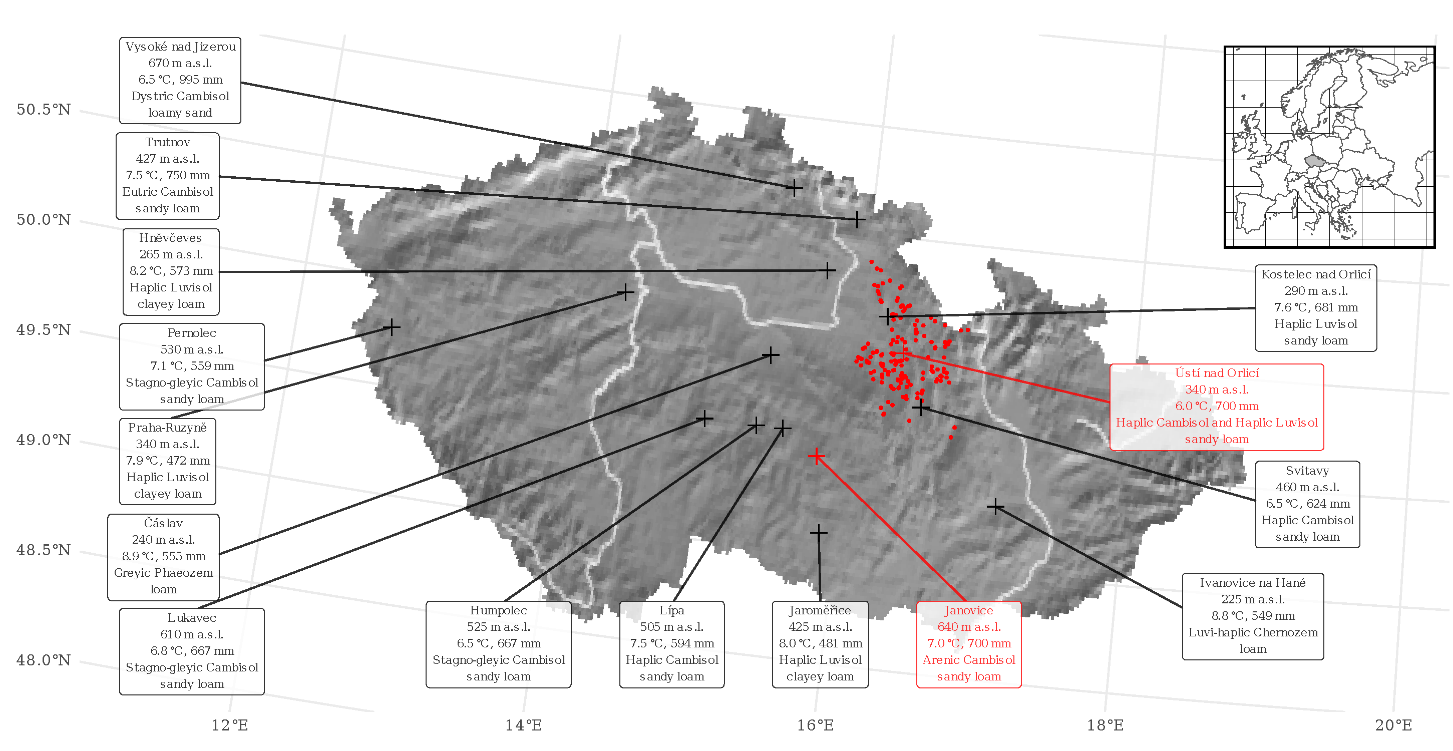
2.1. Site Description and Data Collection

Two groups of soil samples were collected at the territory of the Czech Republic: (1) time series of archived samples obtained from long-term crop trials, which served as a reference library, and (2) samples from two commercial sites, Ústí nad Orlicí and Janovice, as prediction targets of interest (Figure 1). The long-term experiments were maintained by the Crop Research Institute Praha-Ruzyně (CRI) and the Central Institute for Supervising and Testing in Agriculture; their primary focus was fertilization. A brief description can be found in

Table 1. Characteristics of the long-term field experiments.

Experiment a	Est.	Layout b	Crop Rotation c	Reference
CRE	1956	1b × 3t	various (25%)–(WW or TR)–(POT or SB or SM)–(SBA or WW)	[49]
CRT	1984	5b × 1t	WW and SBA (50–100%) complemented with CL, O, PEA, SB, SM	unpublished
FE	1958	1b × 7t	fallow	[50]
FFFE	1979	1b × 6t	(AL or CL)–WW–SM–WW–SBA–(SB or POT)–SBA	[51]
IOSDV	1983	1b × 4t	(SB or POT)–SBA–WBA	[52]
OaMNFE(dc)	2011	1b × 5t	POT–WW–SM–SBA–OSR–WW	[53]
OaMNFE(sf)	1965	1b × 6t	WW–POT–SBA–LCM–WW–POT–O–CL	[54]
RFE	1955	2b × 8t	SW–SB or AL–AL–WW–SB–SBA–POT–WW–SB–SBA	[55]

^a CRE—Crop Rotation Experiment, CRT—Crop Rotation Trial, FE—Fallow Experiment, FFFE—Fraction Factorial Fertilization Experiment, IOSDV—International Long-Term Organic Nitrogen Nutrition Experiments, OaMNFE(dc)—Organic (digestate, compost) and Mineral N Fertilization Experiment, OaMNFE(sf)—Organic (straw, farmyard manure) and Mineral N Fertilization Experiment, RFE—Ruzynĕ Fertilizer Experiment; ^b The number of blocks and treatments per block at each site; ^c AL—alfalfa (Medicago sativa L.), CL—red clover (Trifolium pratense L.), LCM—legume–cereal mixture, O—oat (Avena sativa L.), OSR—winter oilseed rape (Brassica napus L.), PEA—cultivated pea (Pisum sativum subsp. sativum L.), POT—potato (Solanum tuberosum L.), SB—sugar beet (Beta vulgaris subsp. vulgaris L.), SBA—spring barley (Hordeum vulgare conv. distichon (L.) Alef.), SM—maize for silage (Zea mays subsp. mays L.), SW—spring wheat (Triticum aestivum L.), TR—triticale (× Triticosecale Wittm. ex A. Camus.), WBA—winter barley (Hordeum vulgare conv. vulgare L.), WW—winter wheat (Triticum aestivum L.).

. As seen in Table S1, the library was unbalanced with respect to the sample, year, and experimental treatment counts. Topsoil samples from the upper 20 cm were collected using a field shovel following a uniform protocol. The soil was collected from three spots of each plot, and the partial samples were combined into approximately 2 kg lots and homogenized.

Ústí nad Orlicí comprises multiple localities scattered over one district (Figure 1), making it a heterogeneous site. The fields were managed with conventional tillage and sown with winter wheat, winter and spring barley, silage maize, and oilseed rape. The heterogeneity was additionally augmented by an extended timing of the soil sample collection, which took place every spring and fall between 2012 and 2015. About 40 topsoil samples from fields with winter wheat and winter barley were collected by the farmers or their designated persons during each campaign, yielding a total of 335 samples. The commercial site Janovice denotes a single conventionally tilled field, with a crop rotation of silage maize, winter wheat, potatoes, and clover–grass mixture. It contributed 45 topsoil (0–20 cm) samples collected by CRI employees in fall 2017, after the sowing of winter wheat. The sampling points were delimited every 120 m in a way to obtain roughly uniform coverage of the field. There were six partial samples per composite sample of approximately 0.5 kg, which was then homogenized.

The soil samples were dried, sieved through 2 mm mesh, and milled. MIR-DRIFTS spectra were measured using a Thermo Nicolet Avatar 320 FTIR spectrometer with a Ge beam splitter and a TGS detector, equipped with a Smart Diffuse Reflectance accessory (Nicolet, Madison, WI, USA) in a homogeneous mixture of 300 mg bulk soil and 900 mg FTIR grade KBr (Sigma-Aldrich, Darmstadt, Germany) prepared by hand in an agate mortar. Each sample was transferred to a 12 mm diameter diffuse reflectance cup and levelled with a microscope glass slide in a way to avoid compressing mechanically the mixture. Three scans comprising 1869 equidistant bands in the 4002–399 cm⁻¹ wavenumber range were performed, each spectrum was corrected against pure KBr as a background spectrum, and the obtained apparent absorbance (hereafter, absorbance) values averaged to obtain a spectrum with reduced noise [35]. TC content was determined by dry combustion using Vario/CNS analyzer (Elementar Analysensysteme GmbH, Langenselbold, Germany), and hot-water extractable carbon (HWC) content was determined according to Körschens et al. [8] as a measure of SC lability [27,56].

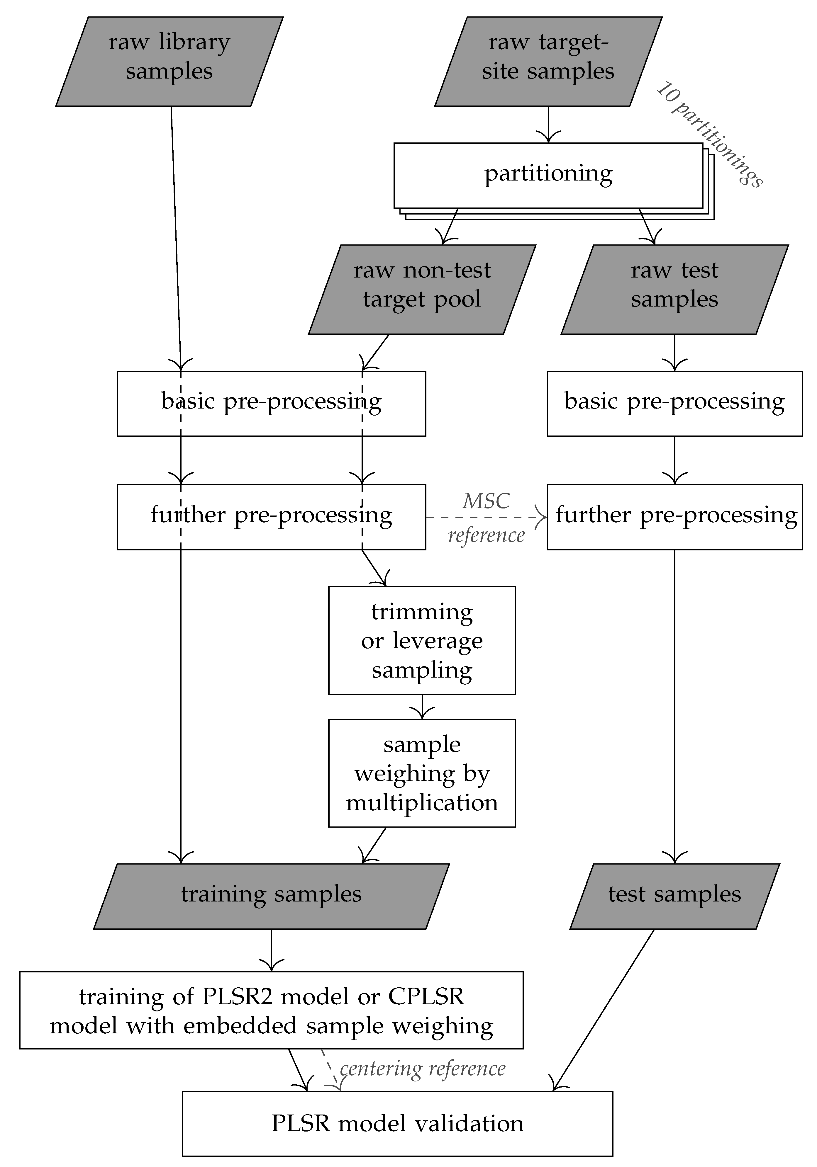
2.2. Data Partitioning and Pre-Processing of MIR-DRIFTS Spectra

The collected data were subjected to a number of pre-processing and subsetting operations, the character of which was differentiated according to the study questions; depending on the scenario, one or more operations could also be omitted. PLSR models for predicting TC and HWC contents from MIR-DRIFTS spectra were then trained, tuned, and validated using the derived datasets. Figure 2 depicts the data processing workflow.

The samples in the library part of the dataset served as the calibration samples in the global (library only) modeling scenario (Figure 3a), equivalent to removal of the “raw non-test target pool”–“sample weighing by multiplication” workflow branch in Figure 2. For each commercial site, 10 independent sets of 12 samples were picked randomly for testing of predictive model quality. The target-site spectra not included in a testing partition made a pool from which samples were picked for model training in other scenarios (Figure 3b,c). The order of samples within these pools was randomized.

Spectral pre-processing was performed before the selection of target-site training samples from the training pools. Noisy bands up to 600 cm⁻¹ [17] and CO₂-affected measurements in the 2268–2389 cm⁻¹ wavenumber range [32] were discarded. For additional signal recovery, the spectra were processed using a moving-average filter with an 11-band window.

In addition to analyzing the resulting spectra, hereafter “raw spectra”, we tested five further pre-processing schemes [57], with each scheme comprising two phases. In the first phase, the moving-average smoothing was either followed with multiplicative scatter correction (MSC) or left unchanged. In the second phase, (1) standard normal variate (SNV), (2) derivative transformation using the Savitzky–Golay filter with third-order polynomial smoothing applied over a moving window of 11 bands, or (3) no transformations were applied to the result. No change to the spectra in both phases was equivalent to removal of the “further pre-processing” box in Figure 2. Initially, continuum removal by dividing the spectrum by its convex hull was also attempted, but it had to be abandoned as extreme outliers were generated. Unlike the remaining transformations, MSC employs information from multiple spectra to derive a common reference spectrum. We were careful to perform this operation using the data in the training spectra pools, exclusively [6,58].

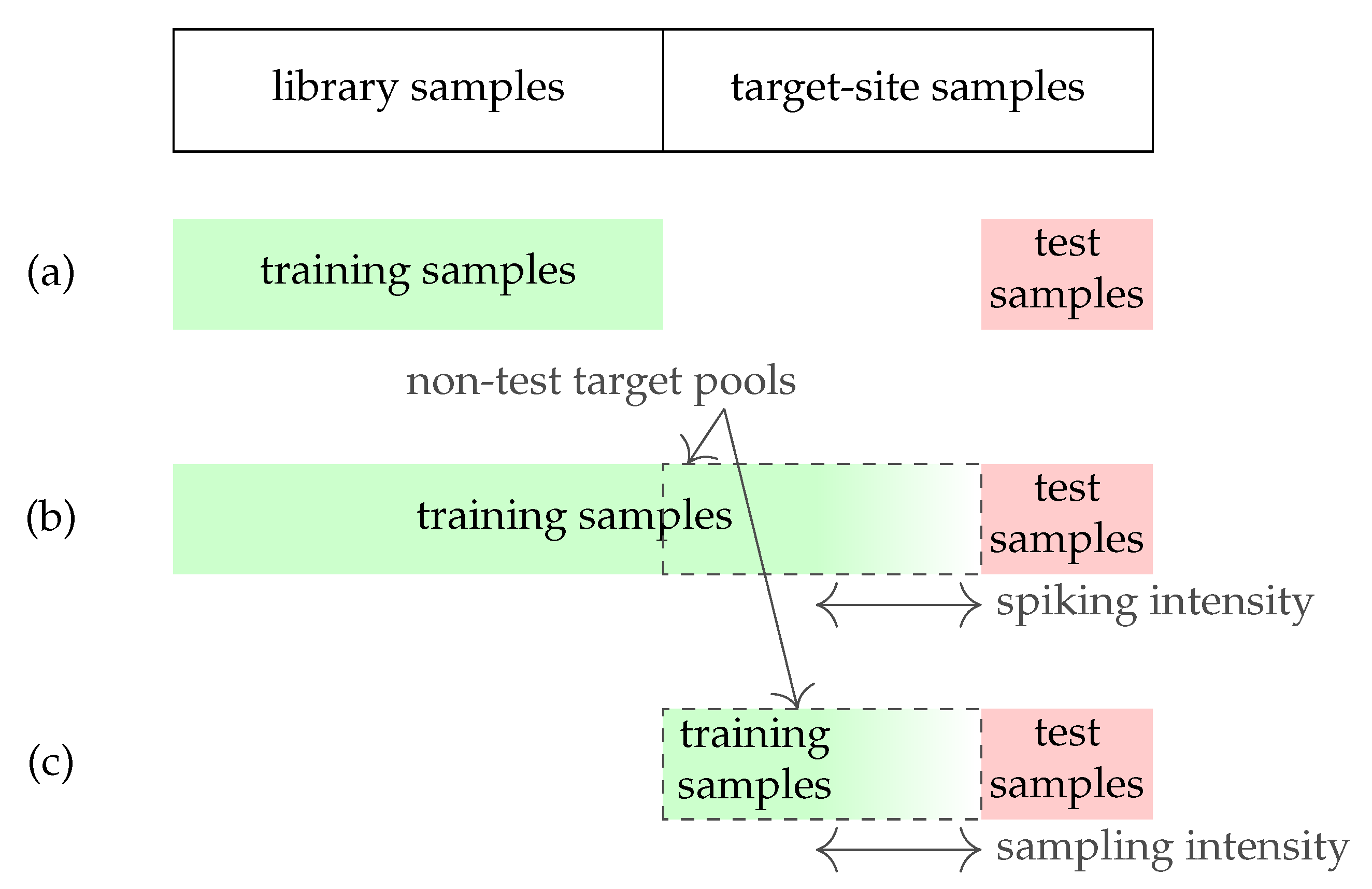
2.3. Calibration Spiking

Calibration spiking was introduced, based on increasing spiking sample counts to the level of 16 samples with a step of 4 samples (Figure 3b). The pre-randomized calibration sample pools were trimmed while preserving the sample orders. In addition to this random scheme, two leverage sampling approaches were assessed: the Kennard–Stone algorithm [59] and conditioned Latin hypercube [60]. The spectra were subjected to PCA prior to the Kennard–Stone algorithm application to reduce the number of dimensions below the sample pool size level.

In order to test for the possibility of a local modeling superiority with respect to models trained both to global and spiked datasets, additional scenarios mirroring the calibration-spiking scenarios but without samples from the long-term experiments were included (Figure 3c). This was equivalent to omitting the “library samples” branch in Figure 2. The training sample selection followed the same three schemes as for calibration spiking, with the same sampling intensity levels.

2.4. Reference Laboratory Data Pre-Processing

TC content cannot exceed a certain level of SC saturation [61,62], whereas HWC cannot be larger than TC. While applying statistical methods to measurements of sample constituents’ concentrations, such as TC and HWC, it is recommended to follow the principles of compositional data analysis. Otherwise, models can yield nonphysical predictions, such as those of negative concentrations, a problem encountered by Baldock et al. [16] and Janik et al. [63], or component sizes the sum of which exceeds 100 %.

Classical statistical tools can be employed to compositional data after subjecting them to log-ratio transformations. Accordingly, three components summing up to the whole soil sample were derived from the TC and HWC measurements: (1) HWC, (2) the part of TC resistant to hot-water extraction (nHWC), and (3) the non-TC part of a sample ($1-\mathrm{TC}$). In the next step, the component values were transformed into two isometric log-ratio (ilr) coordinates according to the formulas [64]:

$${\mathrm{ilr}}_{\mathrm{TC}}=\sqrt{\frac{2}{3}}log\frac{\phantom{{}^{\frac{1}{2}}}{\left(\mathrm{HWC}·\mathrm{nHWC}\right)}^{\frac{1}{2}}}{1-\mathrm{TC}},$$

(1)

$${\mathrm{ilr}}_{\mathrm{HWC}}=\sqrt{\frac{1}{2}}log\frac{\mathrm{HWC}}{\mathrm{nHWC}}.$$

(2)

The ilr_TC coordinate is closely related to TC but accounts for the finite size of a sample, while ilr_HWC can be interpreted as transformed C lability [65]. The latter formulation not only respects the compositional character of the reference data but also avoids confounding lability with TC, thus facilitating their independent analysis. This is unlike raw HWC, the value of which can be affected by both factors [9].

2.5. PLSR Modeling with Unweighed and Weighed Training Samples

The relationship between ilr values and MIR-DRIFTS spectral patterns was modeled using PLSR. Two multiresponse PLSR extensions were trained to both coordinates to account for multivariate character of compositional data [66]. For data partitionings that included both reference-library and target-area samples, the influence of spiking sample weighing was examined by introducing models with 5-fold and 25-fold weighted local observations, in addition to unweighted models. The weighing was performed either in the standard way by data row multiplication—in which case a PLSR2 model [42] was used—or by exploiting the internal weighing capability of the CPLSR model family [47] as a proposed approach. The latter case detoured the “sample weighing by multiplication” Figure 2 workflow step. Obviously, the weighing was restricted to the calibration-spiking scenarios, as the remainder, that is library-only and local-only scenarios, involved only single sources of samples.

Centered values of ilr coordinates were the dependent variables (responses) and centered MIR-DRIFTS intensity values were the independent variables (features) in these models. Like for MSC, the centering was based on information in the training data only. The numbers of PLSR components were tuned using leave-one-out cross-validation with values between 1 and 12 considered. The number of components to keep was determined using one standard error heuristics [67] applied separately to ilr_TC and ilr_HWC RMSECV. In this way, 12,240 bivariate models were calibrated and twice as many tuned models obtained.

The performance of each model was evaluated using test data partitions in terms of R², prediction bias, and RMSEP, followed with RPD_P and RPIQ_P statistics:

$${\mathrm{R}}^2=\frac{V_{Res}\left(0\right)-{\mathrm{RMSEP}}^2}{V_{Res}\left(0\right)},$$

(3)

$$\mathrm{bias}=\frac{{\sum }_{i=1}^n({\widehat{y}}_i-y_i)}{n},$$

(4)

$$\mathrm{RMSEP}=\sqrt{\frac{{\sum }_{i=1}^n{({\widehat{y}}_i-y_i)}^2}{n}},$$

(5)

$${\mathrm{RPD}}_{\mathrm{P}}=\frac{s_{\mathrm{P}}}{\mathrm{SEP}},$$

(6)

$${\mathrm{RPIQ}}_{\mathrm{P}}=\frac{{\mathrm{IQR}}_{\mathrm{P}}}{\mathrm{SEP}},$$

(7)

where $V_{Res}\left(0\right)$—mean square ground truth value, ${\widehat{y}}_i$—predicted ith value, $y_i$—ith ground truth value, n—test sample count, $s_{\mathrm{P}}$—standard deviation of ground-truth values, ${\mathrm{IQR}}_{\mathrm{P}}$—interquartile range of ground-truth values, and $\mathrm{SEP}$—standard error of prediction, which was defined as:

$$\mathrm{SEP}=\sqrt{\frac{{\sum }_{i=1}^n{(\widehat{y_i}-y_i-\mathrm{bias})}^2}{n-1}}.$$

(8)

These were summarized, and the relative influence of the experimental factors on the model performance measures was also examined visually after plotting the relationships.

2.6. Reproducing the Study

The analysis was coded using the R language and executed in the 3.6.2 version of the interpreter [68]. The package vegan (version 2.5.6) [69] was used for PCA, prospectr (0.1.3) [70] and pls (2.7.2) [71] for spectra pre-processing, prospectr and clhs (0.7.2) [72] for leverage sampling, compositions (1.40.3) [73] for ilr transformations, and pls for PLSR modeling. GNU Make [74] was employed for workflow control, and GNU Guix functional package management and containerization capabilities [75] were exploited to obtain reproducible results. The data and code are available from a Zenodo repository (doi:10.5281/zenodo.6337394). Reproduction of the study is going to require the availability of HPC infrastructure. It took approximately three weeks of operation of a 16-CPU virtual machine to complete a full computation cycle and obtain the results.

3. Results

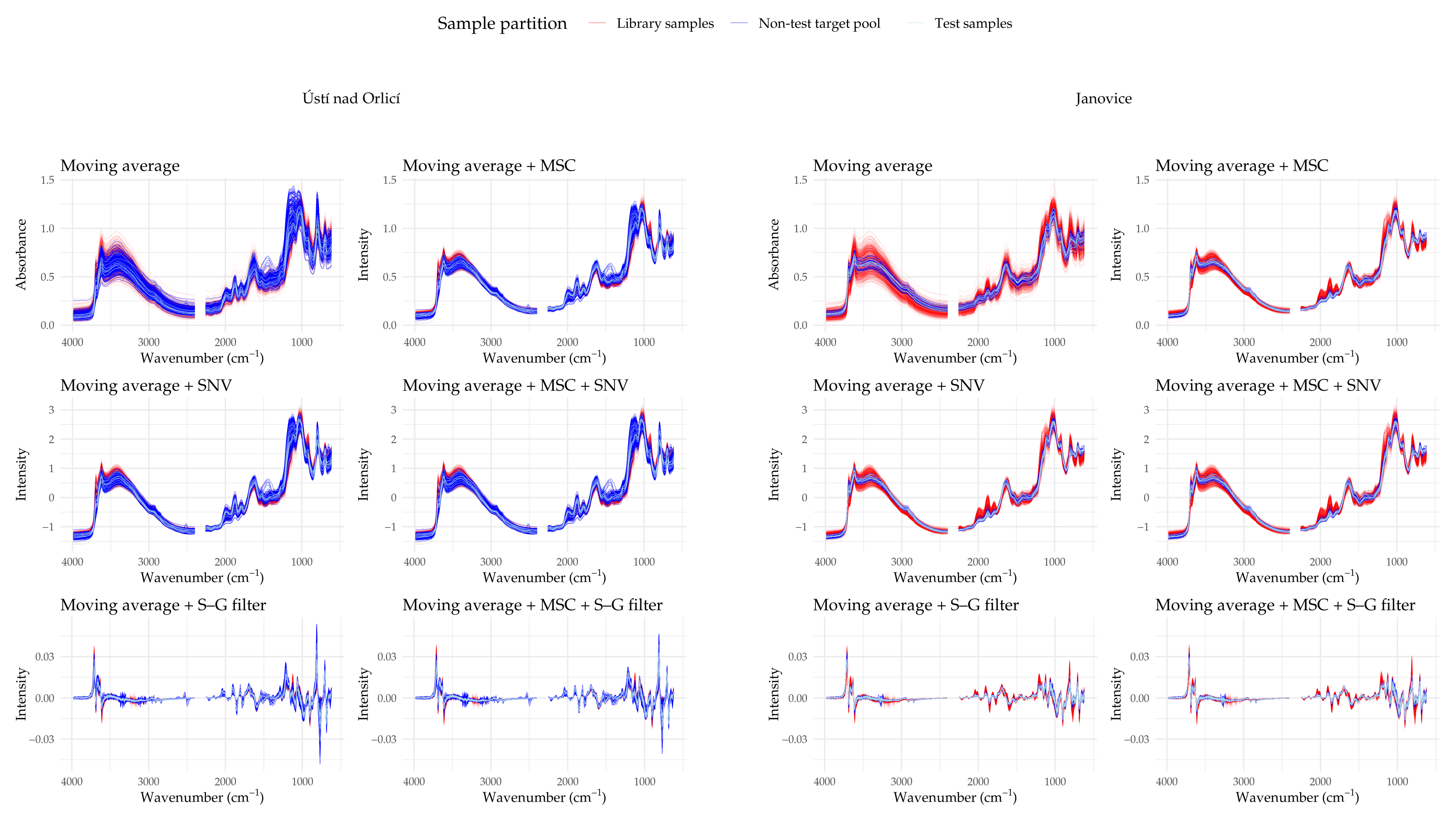
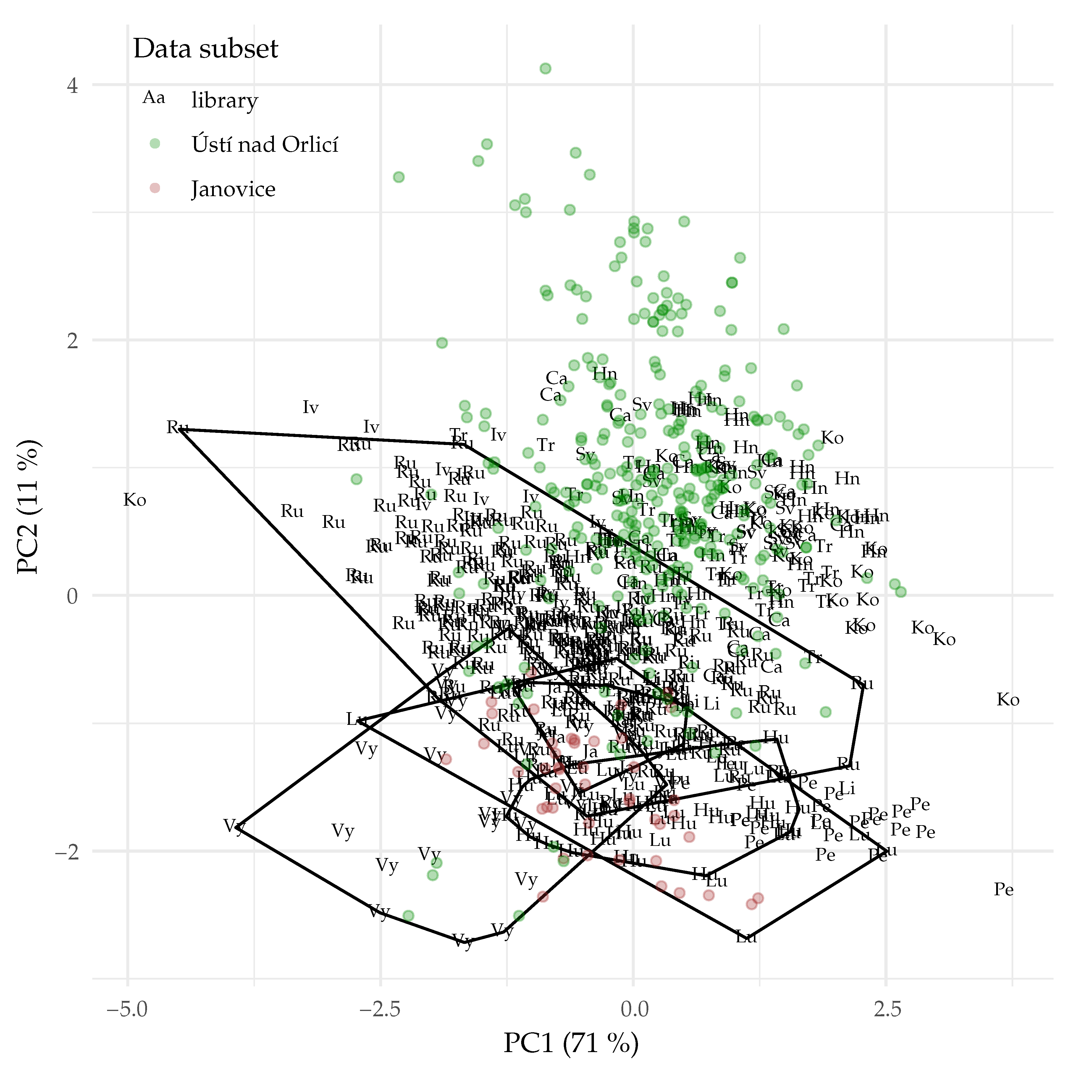
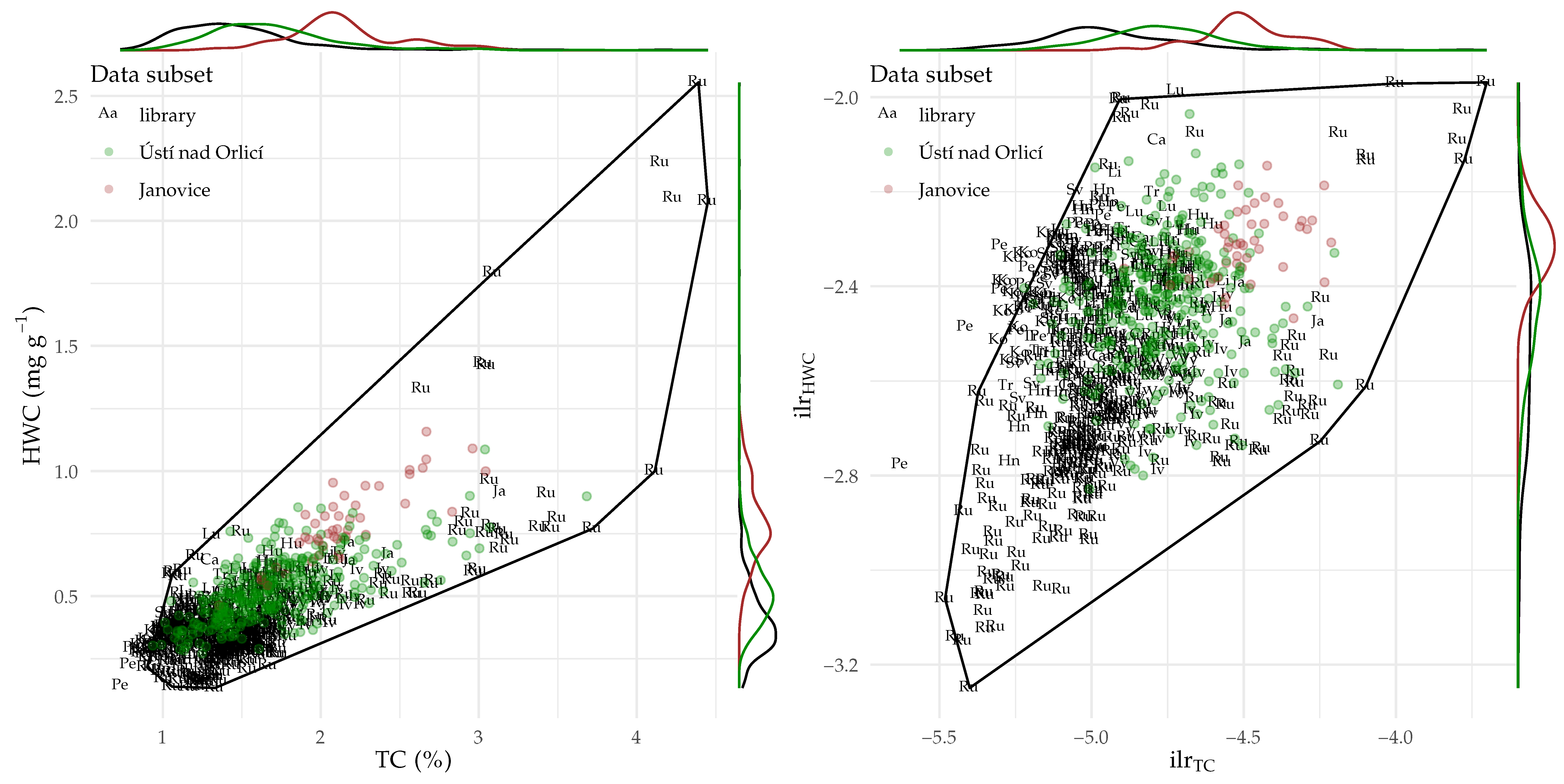
3.1. Patterns in the Raw and Pre-Processed Data

Ústí nad Orlicí spectral signatures were highly varied and, in certain regions, extended beyond the envelope of the library samples regardless of pre-processing (Figure 4 and S3). The scans were subjected to PCA to obtain more insight into the spectral dissimilarity [39]. According to the first two principal component scores, there is substantial overlap between the reference library spectra and Ústí nad Orlicí soil samples, but a significant fraction of the observations occupy the area of the PCA space devoid of library data points due to high PC2 scores (Figure 5). As could be expected, the bulk of high-PC2 library observations represent experimental stations located close to the discussed district, namely Hněvčeves, Svitavy, Čáslav, and Kostelec nad Orlicí (Figure 1). Notable are the large ranges of Ústí nad Orlicí PCA scores, comparable to those of the long-term experiments. In contrast to that pattern, Janovice spectra were enveloped by the library spectra (Figure 4), and the data points form a compact cluster in Figure 5, similar in extent to several individual library sites, as shown using convex-hull polygons.

In addition, the C measurement variation was high in Ústí nad Orlicí and not much smaller than that of the library samples despite the different geographical scales (

Table 2. Location and scale statistics describing the distributions of soil carbon (SC) measurements before and after isometric log-ratio (ilr) transformations.

Statistics	Sample Partition	C Measurement
		Raw		ilr-Transformed
		TC	HWC	ilrTC	ilrHWC
range		(%)	(mg g−1)
	library	0.73–4.45	0.13–2.55	−5.63–−3.70	−3.25–−1.97
	Ústí nad Orlicí	0.94–3.68	0.27–1.09	−5.22–−4.19	−2.83–−2.04
	Janovice	1.35–3.04	0.46–1.16	−4.89–−4.21	−2.47–−2.15
median		(%)	(mg g−1)
	library	1.41	0.38	−4.98	−2.54
	Ústí nad Orlicí	1.65	0.51	−4.77	−2.43
	Janovice	2.10	0.77	−4.51	−2.31
IQR		(pp)	(mg g−1)
	library	0.45	0.16	0.27	0.29
	Ústí nad Orlicí	0.46	0.17	0.23	0.17
	Janovice	0.32	0.16	0.14	0.09
n	library	603
	Ústí nad Orlicí	335
	Janovice	45

and left-hand plot in Figure 6). Both TC and HWC are somewhat shifted upwards relative to the bulk of the reference library. Unlike the PCA scores, the mismatch between target-site C measurements and reference library measurements is more apparent for Janovice. Both TC and HWC are high here, and the only library samples with similar characteristics are a group of Praha-Ruzyně Fallow Experiment experimental plots. A closer examination revealed that those had been assigned to compost fertilization treatments.

Regardless of the data subset, the raw measurements were skewed towards lower values (left-hand plot in Figure 6). The skew, and to a degree high kurtosis, were reduced after the ilr transformations (right-hand plot in Figure 6 and Table S2). Figure 7 depicts the relationships between the raw component values and ilr coordinates. While the TC–ilr_TC relationship is smooth and close to linear, a broken stick pattern was obtained for HWC–ilr_HWC. The outlying samples with HWC in excess of 1.2 mg g⁻¹ all came from Praha-Ruzyně Fallow Experiment plots where compost was applied. Although ilr_TC and ilr_HWC are not simple transformations of, respectively, TC and HWC, as additional components were accounted for in their derivation (Equations (1) and (2)), the relationships are strong enough to permit comparing our results with those reported by authors who had not considered the compositional nature of SC pools.

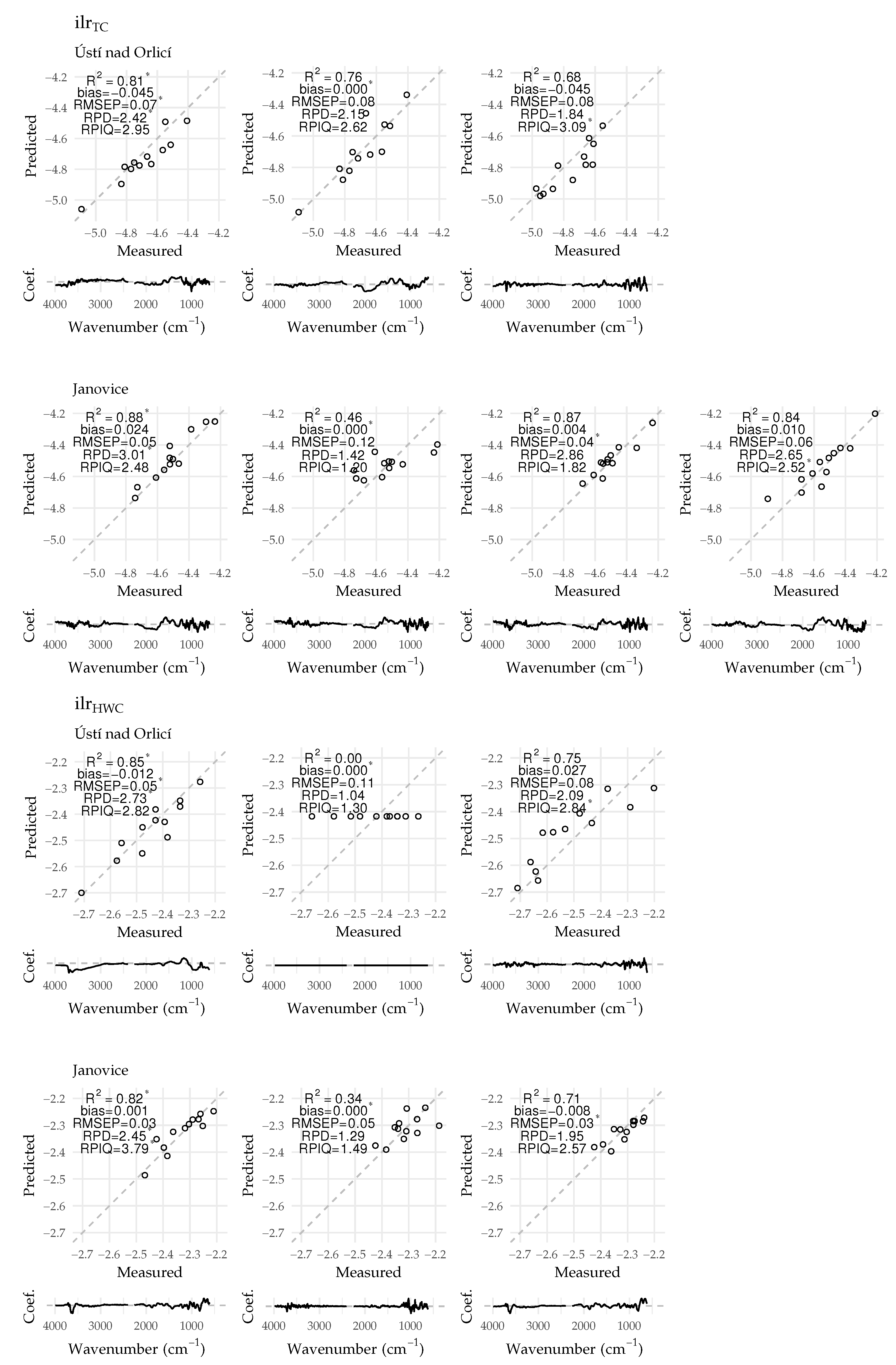
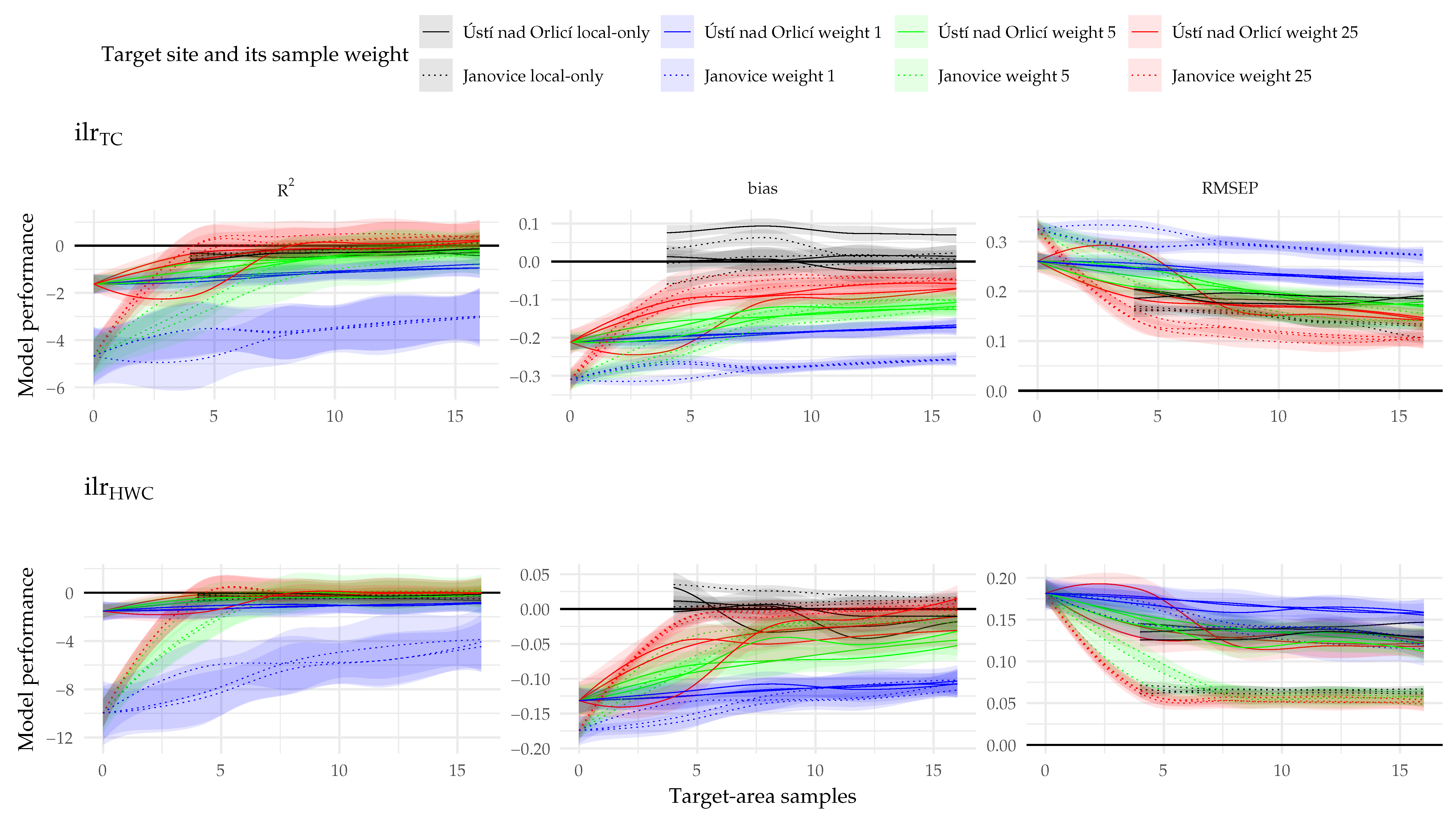
3.2. Accuracy and Precision of the PLSR Models

The predictive performance of the PLSR models varied substantially, as illustrated by the R² statistics (

Table 3. Ranges of PLSR model performance measures according to the dependent variable and the target site. The values outside and inside the brackets correspond to performances obtained for individual data partitionings and performances that were median aggregated across the partitionings, respectively.

Performance Measure	ilrTC		ilrHWC
	Ústí nad Orlicí	Janovice	Ústí nad Orlicí	Janovice
R2	−9.10  [−3.97,  0.33]  0.81	−18.79  [−8.76,  0.57]  0.88	−6.90  [−1.36,  0.18]  0.85	−37.43  [−18.98,  0.35]  0.82
bias	−0.42  [−0.30,  0.16]  0.32	−0.49  [−0.47,  0.07]  0.21	−0.19  [−0.13,  0.07]  0.14	−0.28  [−0.24,  0.04]  0.09
RMSEP	0.07  [0.13,  0.35]  0.51	0.04  [0.08,  0.48]  0.51	0.05  [0.11,  0.19]  0.24	0.03  [0.04,  0.26]  0.29
RPD	0.33  [0.47,  1.27]  2.42	0.23  [0.33,  1.60]  3.01	0.37  [0.68,  1.15]  2.73	0.17  [0.23,  1.29]  2.45
RPIQ	0.30  [0.62,  1.70]  3.09	0.13  [0.26,  1.45]  2.52	0.38  [0.69,  1.26]  2.84	0.18  [0.30,  1.59]  3.79

). Although negative values were obtained for the worst models, models corresponding to R² in excess of 0.80 could be found for each ilr coordinate and target site combination, which is a high quality result according to Janik et al. [20]. However, after aggregating the values across all data partitionings, R² exceeded 0.50, still an unsatisfactory value, only for Janovice while predicting ilr_TC, whereas both ilr_HWC and Ústí nad Orlicí scenarios gave poor results.

The worst negative biases and RMSEP values were comparable, amounting to 0.4–0.5 for ilr_TC and 0.2–0.3 for ilr_HWC. In terms of raw component values, these correspond to approximately 1.30 TC percentage points and 0.09–2.79 mg g⁻¹ HWC, depending on the baseline HWC value (Figure 7). The best models had RMSEP of only 0.04 for ilr_TC (approximately 0.12 pp TC) and 0.03 for ilr_HWC (0.34 mg g⁻¹ HWC for high value range and less for low value range). More conservative estimates, based on partitioning medians, suggested a possibility of predicting ilr_TC with an error of 0.13 (0.38 pp TC) and 0.08 (0.23 pp TC) in Ústí nad Orlicí and Janovice, respectively, while for ilr_HWC, the corresponding values were 0.11 and 0.04 (0.04–1.23 and 0.01–0.45 mg g⁻¹ HWC).

Models with RPD_P or RPIQ_P above 2.5 or even 3.0 were obtained in some scenarios and test data partitions, described in literature as good and excellent predictions [76]. However, typically one should not expect the performance to be higher than 1.7, that is, barely sufficient to estimate the values even as high or low. Unlike for the other measures, Janovice models did not yield consistently superior RPD_P and RPIQ_P relative to Ústí nad Orlicí.

There is an agreement between PLSR regression coefficients of the best Janovice models for predicting ilr_TC regardless of the performance measure in which a model excelled (Figure 8). The pattern is similar to that presented for Baldock et al. [16] square-root transformed TC model, including the presence of aliphatic C−H (at approximately 2890 cm⁻¹), C=O (1740 cm⁻¹), and negative carbonate (1810 cm⁻¹) peaks. In contrast, the coefficients for Ústí nad Orlicí disagree and the pattern is malformed, which may suggest model overfitting. Regression coefficient values are comparable among two of the best-performing Janovice ilr_HWC models. Their patterns do not resemble those published by Zimmermann et al. [17] for labile OC, but these authors modeled raw component sizes, rather than lability, and presented individual PLSR loadings, rather than regression coefficients. There is a major negative peak in the 3700–3600 cm⁻¹ wavenumber range, which corresponds to O−H stretching of clay minerals [77,78]. Other peaks occur at approximately 1000 cm⁻¹ and below. Here, notable is the positive 1050 cm⁻¹ peak, assigned to quartz reflectance [19]. However, according to Nocita et al. [28], the interpretation for the <1000 cm⁻¹ region is challenging due to mineral species vibrations interfering with those of organic molecules. These include iron compounds [13] and carbonates [79]. The peaks do not include 2930 cm⁻¹ and 1620 cm⁻¹ wavenumbers proposed by Demyan et al. [80] for lability assessment. The model minimizing bias behaved differently, and for Ústí nad Orlicí, the smallest-bias model happened to be insensitive to input data variation, which indicates that models should not be selected according to the bias criterion. As with ilr_TC, the pattern is unstable for this latter target site.

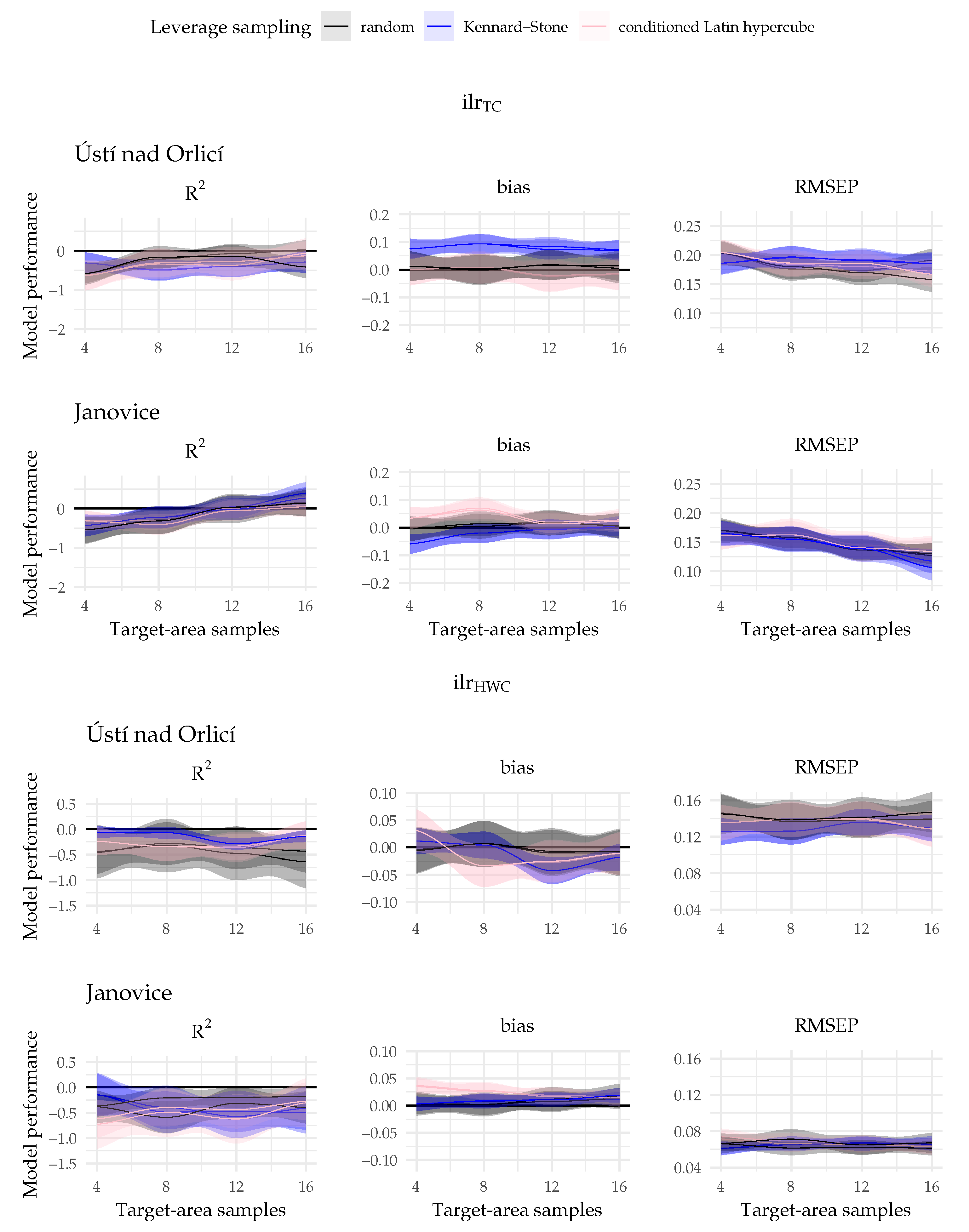
3.3. Factors Affecting PLSR Model Performance

The relationships between the modeling approaches and performance measure values were visualized to identify factors contributing to prediction quality. We present a selection that illustrates the most clear patterns, which, with the exception of the final comparison, is restricted to the models trained to the raw spectra, as the effect of spectra pre-processing was limited. The complete set of visualizations along with input data points can be found in Figure S2.

PLSR models trained to the spectral library, that is, with zero target-site samples, performed poorly, especially for Janovice, as can be seen at the left edge of all plots in Figure 9. Note that this and subsequent figures for legibility depict confidence intervals, whereas ranges are referred to in this section. The R² statistic was negative with the exception of Ústí nad Orlicí ilr_HWC models, in the case of which it ranged between −6.24 and 0.47. The generated predictions were negatively biased, while their imprecision measured by RMSEP exceeded 0.17 units for ilr_TC (about 0.49 pp TC) and 0.08 units for ilr_HWC (0.03–0.89 mg g⁻¹ HWC).

Training of PLSR models to a selection of target-site samples only, while excluding the spectral library, had a clearly positive effect on all measures even with only four training samples, as illustrated by the black lines in Figure 9. However, R² was still negative at this sampling intensity level. Here, predictions for Janovice appear superior to those obtained for Ústí nad Orlicí, especially in terms of RMSEP. Further additions of samples led to more accurate ilr_TC predictions in Janovice, as depicted in more detail in Figure 10. In particular, R² exhibited an increasing trend, with positive values up to 0.88, obtained in a number of scenarios with 16 samples. Prediction improvement of ilr_TC with higher sampling intensity is not so clear for Ústí nad Orlicí. Instead, a pattern of Kennard–Stone leverage sampling inferiority could be discerned, especially in terms of high bias, up to 0.32 units (0.92 pp TC).

RMSEP of ilr_HWC was hardly affected by increasing sampling intensity. On the other hand, a trend towards increased bias can be discerned for Janovice under the random sampling and Kennard–Stone leverage sampling scenarios, but these strategies still do not appear consistently inferior to conditioned Latin hypercube. Positive R² was attained by few and apparently random Janovice models and almost no Ústí nad Orlicí models even at maximum sampling intensity, suggesting a general unsuitability of the local approach to estimating this ilr coordinate.

In Janovice scenarios with PLSR2 models, augmenting the library samples with spike samples yielded results competitive with the local approach when the target-site training samples were given a weight of 25, as shown using red lines in Figure 9. R² up to 0.71 could be attained with only four spiking samples for ilr_TC—in contrast to R² of corresponding local-only models, which was always negative. A notable exception was prediction bias, in the case of which about 85% of the models still underestimated the value of this coordinate. Models with the weight of five (green lines) were competitive with local-only models only in predicting ilr_HWC and only in terms of R² and RMSEP. More spiking samples were required to obtain a desirable effect than with 25-fold spiking sample weighing. The superiority of global Ústí nad Orlicí models relative to Janovice vanished or became inversed as spike samples were added to training datasets. The performance remained better only in scenarios without spike sample weighing (blue lines), but here the prediction quality was poor for both target sites, making this class of scenarios not interesting.

Leverage sampling had little effect on the quality of models that involved spiked library spectra, but the performance measures responded to the choice between PLSR2 and CPLSR family (Figure S3). The application of the CPLSR method was clearly detrimental for the prediction quality of both ilr_TC and ilr_HWC in Janovice samples compared to the standard approach. In the case of Ústí nad Orlicí, the effect of replacing PLSR2 with CPLSR was not so strong, but it still appears negative. The limited sensitivity of model performance to spectra pre-processing can be illustrated by two favorable combinations of spectra selection and weighing strategies. As depicted in Figure S4, systematic prediction quality differences are hard to discern except for the uninteresting library-only scenario, where all models failed.

4. Discussion

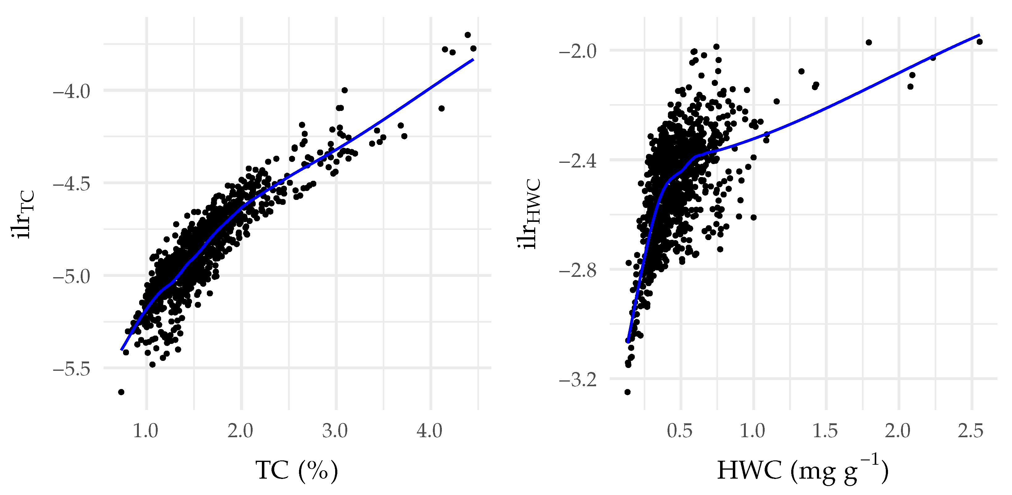
4.1. Distributional Data Properties and the Effect of Log-Ratio Transformation

The high scatter of observations in PCA (Figure 5) and SC (Figure 6) measurements, comparable in extents to those of long-term experiments, indicates high spatial heterogeneity of Ústí nad Orlicí district soils. This pattern corroborates the need for dense soil sampling to map and monitor SC in the conditions of the Czech Republic and, arguably, beyond [3,4], from which the need to develop cost-effective assessment methods follows [4]. However, in addition to the variability of soil properties, non-uniform sampling techniques might have also been a contributing factor, as unlike in the remaining campaigns, the task was relegated to farmers. In contrast to that, the relative compactness of the Janovice PCA cluster corresponds to the fact that the data collection was constrained to a single field. The high TC and HWC contents encountered at this locality might have been related to long-term organic fertilization of this field.

High performance of a PLSR model can be attained when the predicted variable has a Gaussian distribution, and in chemometric studies, it is common to transform target measurements [13]. Stenberg et al. [6] highlighted skewness of organic matter concentrations in cropland soil samples towards low values, a common pattern that can contribute to prediction bias [34]. Normalization of such data can be attained by applying a square-root [16,20,39] or a logarithmic [81,82,83] transformation. However, while these bound the predictions to be above zero [16], the maximum values remain unbounded.

A log-ratio affects the shape of data distribution like the above transformations, but in addition to that, back-transformed predictions correspond to physical reality for compositional components [64]. The present study demonstrates improved skewness and kurtosis of ilr coordinates relative to raw component concentrations (Figure 6) and provides evidence of compatibility of log-ratios with PLSR predictive modeling. The proposed data analysis approach could be refined in the future by accounting for carbon saturation limits [61,62] in the ilr transformation. Another potential extension would be to consider also the spectral measurements as compositional [84].

4.2. Absolute Performance of the Predictive Models

The top R² conservative estimate of only 0.57 when predicting ilr_TC and low RPD_P and RPIQ_P evaluations (Table 3) do not corroborate the purported potential of MIR-DRIFTS to become a cost-effective yet reliable laboratory method for SC assessment [13,25,35]. The agreement between the PLSR regression coefficient patterns obtained in the present study (Figure 8) and reported in literature [16,33,81] rules out major errors during both reference data collection and sample scanning and subsequent data analysis. Barra et al. [22] and Bellon-Maurel and McBratney [26] summarized model quality estimates for predicting OC and TC from MIR spectra. Although high-performing models prevail in reported research, a number of SC studies suffer from methodological issues that arguably bias the results towards higher accuracy. For example, Zimmermann et al. [17] employed a systematic rather than random validation sample and, moreover, included the validation data in PLSR model tuning dataset. More recently, Zhang et al. [18] erroneously [23] considered optimistic bias of model cross-validation results as an advantage and did not present the obtained independent validation statistics. It can be presumed that the models performed not so satisfactorily on the test datasets. Deiss et al. [31] contrasted the performance of PLSR and support vector machine models to predict OC in soil samples from two sites. Despite testing multiple combinations of spectral pre-processing and modeling scenarios, the authors presented only the performance measures of their best models. Those happened to be comparable to our top-rated results. In addition, their selection was based on full-validation statistics, which draws an over-optimistic picture of MIR-DRIFTS potential for real-life applications, where only few or even no validation samples would be available.

Methodological issues aside, not all models have been reported to perform well. The Bellon-Maurel and McBratney [26] review includes formulations that resulted in modest RPD_P values, similar to those obtained in the present study. In the more recent Page et al. [10] work, MIR-DRIFTS substantially underestimated OC loss over time in a long-term experiment, similar to our negative ilr_TC biases. Moreover, the estimated effect of evaluated management treatments contradicted that which was inferred using traditional OC determination. Calderón et al. [85] predicted OC in several crop experiments using PLSR and obtained RMSEP of 0.67–0.80 pp; that is beyond our upper RMSEP conservative bracket for TC. More research, preferably based on cooperation between multiple spectroscopy laboratories, is needed to determine to what degree different prediction performance results across studies can be attributed to the training samples at hand [29], sample preparation and scanning process differences [13,25,29], reference laboratory effect [13,29], or predictive model family and calibration workflow [13,25].

The fragility of MIR-DRIFTS to assess SC is further illustrated by C lability prediction performance. The negative 3650–3600 cm⁻¹ and positive 1050 cm⁻¹ Janovice PLSR regression coefficient peaks (Figure 8) can be related to the protective function of clay minerals with respect to soil organic matter [7,62]. However, with the majority of the remaining major peaks located in the <1000 cm⁻¹ region, the predictions are prone to noise introduced by variation in soil mineralogy [28]. Also in the area of lability assessment, studies with over-optimistic results can be found. Our best ilr_HWC calibrations performed similarly in terms of R² and RPD_P to the PLSR models developed by Zhang et al. [27] for predicting raw HWC. Like Deiss et al. [31], these authors presented only their top-performing models for each investigated scenario, and in addition to that, they did not employ an independent test dataset, reporting only cross-validation statistics. Yang et al. [86] adopted a similar approach for the prediction of particulate organic carbon (POC), with comparable outcomes. Zimmermann et al. [17] attempted to predict two labile pools and reported RPD_P of only 2.0 for dissolved OC. Although the correlation between predicted and measured values was satisfactory and particulate organic matter was predicted with high accuracy, there was an information leak from the validation dataset while training of their models. A similar error was made by Calderón et al. [85] while tuning PLSR models for permanganate oxidizable carbon (POXC) predictions in a study that reported a high R² of about 0.8.

One factor contributing to prediction performance deterioration of all of the present study’s models was probably the noise introduced to the spectra by grinding the soil samples by hand. Stumpe et al. [87] demonstrated that long grinding can reduce undesirable MIR spectra random variability. However, uniform grinding, a condition not attainable with a manual operation, turned out to be even more important for OC prediction quality. The importance of controlled grinding in a MIR spectroscopy workflow is acknowledged also by other authors [13,16,33]. Particle size differences, a problem related to soil sample grinding [26,87], generate undesirable baseline shifts [88]. Many workers [80,85,86], including those reporting highly accurate predictions [16,27,32,63], routinely apply baseline correction to their measurements. Although we tested several combinations of spectral pre-processing workflows, this step was not included in the present study, which might have contributed to scanning artifacts remaining in the data. However, methods such as MSC and Savitzky–Golay derivation also address baseline variations [58], yet we were unable to associate them with systematic prediction improvement (Figure S4). According to Du and Zhou [24], moving average can diminish information in absorbance features, so perhaps we should have avoided it as a routine pre-processing step to remove noise.

The attempt to predict total, rather than organic, C probably also impaired the obtained results. In addition to OC, TC includes carbonates as a major C source, which have a different spectral profile, potentially interfering with the OC signal [17,25,88]. In the present study, the Praha-Ruzyně is a site with moderate carbonate content. Although average topsoil pH does not exceed seven, carbonates are visible by eye in a deeper soil layer. Moreover, the locality included experimental plots with compost amendments, which were associated with atypical C patterns (Figure 6). A compost fertilization experiment disrupted PLSR prediction quality also in the Calderón et al. [85] study. The authors reported an improvement after removing the problematic site from the dataset, and it is possible that a similar effect would be obtained in the present study. Perhaps, with OC being modeled instead of TC, PLSR regression coefficient peaks would have avoided the <1000 cm⁻¹ region, hypothesized to interfere with ilr_HWC predictions (Figure 8).

Some errors might have been related to insufficient sample dilution with KBr [89], especially for Ústí nad Orlicí spectra, which lied outside of the long-term experiments envelope primarily in the high-absorbance zone (Figure 4). This region coincided with the 1280–1070 cm⁻¹ wavelength range associated with the silicate inversion feature that can interfere with carbonates signal below a certain dilution level [88]. However, Demyan et al. [80] did not confirm this effect and, instead, associated strong dilutions with the absence of certain absorption features. The traditional view on the need to mix soil samples with KBr for MIR-DRIFTS has been put into question also by Reeves III [25], and according to Tinti et al. [89] and Reeves [90], it can even have a negative effect. Perhaps, then, it would have been preferable to use neat samples in the present experiment.

Inferior ilr_HWC fit relative to ilr_TC might have been related to low HWC concentrations in the soil samples. Measurements of such minute pools tend to be more affected by external conditions than those of major components [17,27]. Although HWC appears in both ilr formulas, one can argue that a ratio, as employed for ilr_HWC (Equation (2)), is more sensitive to error than a geometric mean in the ilr_TC formula (Equation (1)).

4.3. Model Performance with Individual Training Data Subsets

In addition to the Praha-Ruzyně issue, the obtained poor performance of global scenarios can be attributed to the calibration domain mismatch between the library samples collected from long-term experiments and those collected at the target sites (Figure 5 and Figure 6). Especially in the case of Janovice, notable are the high TC and HWC contents, which explain the strong negative bias in the predictions [26]. The negative influence of OC mismatch across datasets on its predictions was demonstrated by Seidel et al. [30] with VisNIR and by Guerrero et al. [39] with NIR spectroscopy.

The reference spectra in the experiment comprise long time series of observations but represent a limited number of locations. Similarly, Zhang et al. [27] obtained their samples from a limited number of long-term experiments, and their reported results are similar to ours. Various authors stress an importance of long-term experiments for studying SC, especially in the context of the low rates of its quantitative changes [3,5,11]. Nevertheless, maximizing the geographical extent of the reference data should apparently be prioritized for predicting a factor with a high spatial variability, as it is the case for SC and its fractions [3,4,5]. A number of studies that adopted this strategy [16,20,33,35,82] demonstrate that high-quality predictive models can be developed in this way.

These issues do not apply to the local-only models, which do not involve any library spectra and a possibility of calibration domain mismatch is largely eliminated. Superior predictions characterizing locally calibrated PLSR models in the present study can be in part linked to the absence of Praha-Ruzyně samples in the training dataset, analogously to the effect observed by Calderón et al. [85] after training a model without an atypical site found in their data. This strategy largely removed ilr_TC prediction bias in our study (Figure 9), corroborating the calibration domain mismatch problem related to the reference library. However, the model quality was still unsatisfactory, especially for ilr_HWC, perhaps due to the limited sizes of the training data. The importance of a sufficient sample size was demonstrated by Guerrero et al. [39] in a NIR study and by Brown [91] in a VisNIR study, where the obtained performance approached that of calibration-spiking models only when large numbers of training samples were available. The costs and uncertain results involved in such a scenario make the advantage of spectroscopic estimation over standard oxidation methods questionable. According to Soriano-Disla et al. [13], local models are particularly suitable at small spatial scales with homogeneous sites. This condition may explain why the predictions for Janovice were superior and responded better to sampling intensity increase (Figure 10) relative to Ústí nad Orlicí. In particular, it might have been related to the smaller range of C measurements from this more homogeneous target site. After accounting for this effect, the prediction quality superiority was not apparent, anymore, as illustrated by the RPD_P and RPIQ_P statistics.

Calibration spiking avoids an excessive reduction of training dataset sizes, and some of the best models in the present study could be associated with this strategy. A generally consistent positive relationship between the sampling and spiking intensity and PLSR model performance was obtained across the scenarios. It is similar to the OC prediction pattern with NIR spectroscopy obtained by Guerrero et al. [39] while increasing the number of target samples from 8 to 16 and 32. Analogously to the ilr_HWC pattern in the present study, Janik et al. [20] reported improved POC prediction quality with both calibration-spiking and local post-hoc models relative to unsatisfactory library-only predictions. The weaker effect of spiking on the performance of Ústí nad Orlicí models than for Janovice can, again, be explained by the high spectral variation of the geographically scattered samples, a situation described by Cezar et al. [36] in an experiment with ASD Fieldspec measurements.

An interest in calibration spiking is motivated by economical and environmental reasons [36]. Accordingly, satisfactory results should be expected even with a modest number of spiking samples [38]. The prediction improvement equivalent to maximizing the spiking intensity, but obtained by mere introduction of additional copies of the target-site data points, as observed for Janovice, is encouraging in this regard. It is also in line with our hypothesis on the potential of calibration spiking to reduce the number of samples for which laboratory reference data need to be obtained. Similarly, Guerrero et al. [39] reported that, for some target sites and a baseline spiking intensity of 8 samples, 25-fold weighing had a stronger positive effect on OC prediction quality than increasing the spiking sample number to 16 or 32. Perhaps further improvement would have been obtained with even heavier weights. However, Stork and Kowalski [40] tested weights up to 70 and determined an optimal number of spike sample copies as 24 in one scenario and less in the remainder, according to the Hotelling’s T² statistics. In recent years, possibilities of predicting SC from MIR spectra collected in field rather than laboratory conditions without sample pretreatment have been explored [92]. Studies are needed to find out whether the positive influence of calibration spiking replicates in this more challenging setting.

4.4. The Effect of Leverage Sampling and Evidence against the CPLSR Internal Weighing Superiority Hypothesis

Clairotte et al. [33] and D’acqui et al. [81] reported OC prediction improvement with MIR-DRIFTS spectroscopy when leverage sampling was employed. In the present study, no apparent systematic differences were obtained with respect to the prediction performance among the random spiking and the spiking spectra selection based on conditioned Latin hypercube. The Kennard–Stone algorithm, on the other hand, was associated with biased ilr_TC predictions in Ústí nad Orlicí scenarios. This leverage sampling scheme tends to pick distant observations, located at the edges of a hyperspace (Figure S5). It also operates incrementally, as opposed to conditioned Latin hypercube, in the case of which the spectra are picked at once and can be more representative of a dataset [83]. Kennard–Stone application to the heterogeneous Ústí nad Orlicí dataset might have yielded outlier spiking samples, perhaps corresponding to soils with atypical textures [87] or mineralogy [85]. Ng et al. [83] obtained unstable calibrations involving this scheme except for large training samples. This apparent unreliability of the Kennard–Stone algorithm for small sample sizes relative to the size and heterogeneity of a target area puts in question its usability in campaigns aimed at minimizing reference data collection effort to obtain cost-effective predictions.

Internal weighing capability of the CPLSR extension of PLSR [47] was tested as an alternative to the spiking set augmentation by data point copies. Contrary to our hypothesis, the obtained models performed poorly, especially for Janovice. Sankey et al. [41] attempted to predict SC from VisNIR spectral data using boosted regression trees for different levels of local sample weights relative to the weights of the samples in the reference library. The authors expressed skepticism with respect to their results, in which the model performance decreased substantially for one target site, and while a positive relationship was observed for another, the obtained improvement was modest. Still, given the limited number of studies devoted to the topic so far, it seems worthwhile to further explore effects of embedded weighing with other data and other classes of predictive models [31,63].

5. Conclusions

Log-ratio transformation of laboratory reference measurements is recommended to avoid non-physical predictions, separate confounding factors, and improve data distributional properties. Accounting for carbon saturation limits and treating spectral measurements as compositional are potential further refinements of this approach.

Conservative estimates of PLSR model performances were lower than the values typically reported for MIR-DRIFTS SC predictions. This discrepancy could be attributed to the noise in the data introduced by manual sample grinding, their inadequate dilution with KBr, presence of an atypical site with carbonate soil and compost fertilization in the spectral library, the library’s insufficient geographical coverage, and calibration domain mismatch relative to the validation samples. It was also in part explained by optimistic bias encountered in the literature due to preference of cross-validation over independent model validation, information leaks from training to testing datasets, and presenting only top-performing validated models by certain authors. There is a need for international cooperation to identify leverage points that could improve reliability of MIR-DRIFTS SC assessments, standardize data collection and treatment workflows, harmonize spectral libraries, and facilitate their use.

Target-site comparison revealed differences in sample heterogeneity related to uneven geographical extents and, possibly, varied soil sampling protocols where farmers were involved. Not enough representative training data were available to satisfactorily predict soil C properties in the more geographically extensive district-scale dataset. Here, spectral and reference laboratory data variation was similar to that of the data from more scattered long-term experiments, corroborating a need for a dense sampling grid to monitor soil C and concerns about potential costs involved.

Predicting soil properties at a field scale removed the issues related to the reference library. Although some models performed very well, the quality was unstable with respect to the choice of validation data even with an application of leverage selection algorithms. C lability predictions were especially fragile, presumably due to the small size of the hot-water extractable pool. The quality of field-scale models responded positively to increasing sampling intensity in local-only scenarios, but further additions of samples in an attempt to obtain more representative training datasets would have been incompatible with the aim of reducing reference laboratory analysis expenses.

Calibration spiking combined with PLSR2 modeling was associated with a steep increase of model quality as additional target-site calibration samples were added, especially in combination with heavy weighing. It, therefore, appears to be a promising cost-effective and environmentally friendly SC monitoring solution but only under the assumption that the available spectral library accounts to a sufficient degree for soil variability. A similar effect could not be obtained with CPLSR models and embedded weighing enabled by this PLSR extension. Although prediction performance was poor in the present study, the internal weighing approach may still be worth testing with other multivariate model families. A training-sample size constraint was encountered while applying Kennard–Stone leverage sampling to the heterogeneous district-scale dataset, and it appears that application of this algorithm is not compatible with the aim of reducing costs of SC assessments.

References

1. Reeves, D. The role of soil organic matter in maintaining soil quality in continuous cropping systems. Soil Tillage Res. 1997, 43, 131–167. [Google Scholar] [CrossRef]
2. Bünemann, E.K.; Bongiorno, G.; Bai, Z.; Creamer, R.E.; De Deyn, G.; De Goede, R.; Fleskens, L.; Geissen, V.; Kuyper, T.W.; Mäder, P.; et al. Soil quality—A critical review. Soil Biol. Biochem. 2018, 120, 105–125. [Google Scholar] [CrossRef]
3. Smith, P.; Soussana, J.F.; Angers, D.; Schipper, L.; Chenu, C.; Rasse, D.P.; Batjes, N.H.; Van Egmond, F.; McNeill, S.; Kuhnert, M.; et al. How to measure, report and verify soil carbon change to realize the potential of soil carbon sequestration for atmospheric greenhouse gas removal. Glob. Chang. Biol. 2019, 26, 219–241. [Google Scholar] [CrossRef] [PubMed] [Green Version]
4. Paustian, K.; Collier, S.; Baldock, J.; Burgess, R.; Creque, J.; DeLonge, M.; Dungait, J.; Ellert, B.; Frank, S.; Goddard, T.; et al. Quantifying carbon for agricultural soil management: From the current status toward a global soil information system. Carbon Manag. 2019, 10, 567–587. [Google Scholar] [CrossRef] [Green Version]
5. Batjes, N.H.; Van Wesemael, B. Chapter Measuring and Monitoring Soil Carbon. In Soil Carbon: Science, Management and Policy for Multiple Benefits; Banwart, S.A., Noellemeyer, E., Milne, E., Eds.; CAB International: Wallingford, UK, 2015; Volume 71, pp. 188–201. [Google Scholar]
6. Stenberg, B.; Rossel, R.A.V.; Mouazen, A.M.; Wetterlind, J. Visible and Near Infrared Spectroscopy in Soil Science. In Advances in Agronomy; Elsevier: Amsterdam, The Netherlands, 2010; Volume 107, pp. 163–215. [Google Scholar] [CrossRef] [Green Version]
7. Kan, Z.R.; Liu, W.X.; Liu, W.S.; Lal, R.; Dang, Y.P.; Zhao, X.; Zhang, H.L. Mechanisms of soil organic carbon stability and its response to no-till: A global synthesis and perspective. Glob. Chang. Biol. 2021, 28, 693–710. [Google Scholar] [CrossRef]
8. Körschens, M.; Schulz, E.; Behm, R. Heißwasserlöslicher C und N im Boden als Kriterium für das N-Nachlieferungsvermögen. Zentralblatt Für Mikrobiol. 1990, 145, 305–311. [Google Scholar] [CrossRef]
9. Thomas, B.W.; Whalen, J.K.; Sharifi, M.; Chantigny, M.; Zebarth, B.J. Labile organic matter fractions as early-season nitrogen supply indicators in manure-amended soils. J. Plant Nutr. Soil Sci. 2016, 179, 94–103. [Google Scholar] [CrossRef]
10. Page, K.; Dalal, R.; Dang, Y. How useful are MIR predictions of total, particulate, humus, and resistant organic carbon for examining changes in soil carbon stocks in response to different crop management? A case study. Soil Res. 2013, 51, 719–725. [Google Scholar] [CrossRef]
11. Haynes, R. Labile Organic Matter Fractions as Central Components of the Quality of Agricultural soils: An Overview. Adv. Agron. 2005, 85, 221–268. [Google Scholar] [CrossRef]
12. Sanderman, J.; Hengl, T.; Fiske, G.J. Soil carbon debt of 12,000 years of human land use. Proc. Natl. Acad. Sci. USA 2017, 114, 9575–9580. [Google Scholar] [CrossRef] [Green Version]
13. Soriano-Disla, J.M.; Janik, L.J.; Viscarra Rossel, R.A.; Macdonald, L.M.; McLaughlin, M.J. The Performance of Visible, Near-, and Mid-Infrared Reflectance Spectroscopy for Prediction of Soil Physical, Chemical, and Biological Properties. Appl. Spectrosc. Rev. 2014, 49, 139–186. [Google Scholar] [CrossRef]
14. Bongiorno, G.; Bünemann, E.K.; Oguejiofor, C.U.; Meier, J.; Gort, G.; Comans, R.; Mäder, P.; Brussaard, L.; De Goede, R. Sensitivity of labile carbon fractions to tillage and organic matter management and their potential as comprehensive soil quality indicators across pedoclimatic conditions in Europe. Ecol. Indic. 2019, 99, 38–50. [Google Scholar] [CrossRef]
15. Gregorich, E.; Carter, M.; Angers, D.; Monreal, C.; Ellert, B. Towards a minimum data set to assess soil organic matter quality in agricultural soils. Can. J. Soil Sci. 1994, 74, 367–385. [Google Scholar] [CrossRef] [Green Version]
16. Baldock, J.; Hawke, B.; Sanderman, J.; Macdonald, L. Predicting contents of carbon and its component fractions in Australian soils from diffuse reflectance mid-infrared spectra. Soil Res. 2013, 51, 577–595. [Google Scholar] [CrossRef] [Green Version]
17. Zimmermann, M.; Leifeld, J.; Fuhrer, J. Quantifying soil organic carbon fractions by infrared-spectroscopy. Soil Biol. Biochem. 2007, 39, 224–231. [Google Scholar] [CrossRef]
18. Zhang, L.; Yang, X.; Drury, C.; Chantigny, M.; Gregorich, E.; Miller, J.; Bittman, S.; Reynolds, D.; Yang, J. Infrared spectroscopy prediction of organic carbon and total nitrogen in soil and particulate organic matter from diverse Canadian agricultural regions. Can. J. Soil Sci. 2018, 98, 77–90. [Google Scholar] [CrossRef] [Green Version]
19. Calderón, F.J.; Reeves, J.B.; Collins, H.P.; Paul, E.A. Chemical Differences in Soil Organic Matter Fractions Determined by Diffuse-Reflectance Mid-Infrared Spectroscopy. Soil Sci. Soc. Am. J. 2011, 75, 568–579. [Google Scholar] [CrossRef] [Green Version]
20. Janik, L.J.; Skjemstad, J.; Shepherd, K.; Spouncer, L. The prediction of soil carbon fractions using mid-infrared-partial least square analysis. Soil Res. 2007, 45, 73–81. [Google Scholar] [CrossRef] [Green Version]
21. Gredilla, A.; De Vallejuelo, S.F.O.; Elejoste, N.; De Diego, A.; Madariaga, J.M. Non-destructive Spectroscopy combined with chemometrics as a tool for Green Chemical Analysis of environmental samples: A review. TrAC Trends Anal. Chem. 2016, 76, 30–39. [Google Scholar] [CrossRef]
22. Barra, I.; Haefele, S.M.; Sakrabani, R.; Kebede, F. Soil spectroscopy with the use of chemometrics, machine learning and pre-processing techniques in soil diagnosis: Recent advances–A review. TrAC Trends Anal. Chem. 2021, 135, 116166. [Google Scholar] [CrossRef]
23. Armenta, S.; De la Guardia, M. Vibrational spectroscopy in soil and sediment analysis. Trends Environ. Anal. Chem. 2014, 2, 43–52. [Google Scholar] [CrossRef]
24. Du, C.; Zhou, J. Evaluation of Soil Fertility Using Infrared Spectroscopy—A Review. In Climate Change, Intercropping, Pest Control and Beneficial Microorganisms; Springer: Dordrecht, The Netherlands, 2009; pp. 453–483. [Google Scholar] [CrossRef]
25. Reeves III, J.B. Near- versus mid-infrared diffuse reflectance spectroscopy for soil analysis emphasizing carbon and laboratory versus on-site analysis: Where are we and what needs to be done? Geoderma 2010, 158, 3–14. [Google Scholar] [CrossRef]
26. Bellon-Maurel, V.; McBratney, A. Near-infrared (NIR) and mid-infrared (MIR) spectroscopic techniques for assessing the amount of carbon stock in soils—Critical review and research perspectives. Soil Biol. Biochem. 2011, 43, 1398–1410. [Google Scholar] [CrossRef]
27. Zhang, L.; Yang, X.; Drury, C.; Chantigny, M.; Gregorich, E.; Miller, J.; Bittman, S.; Reynolds, W.D.; Yang, J. Infrared spectroscopy estimation methods for water-dissolved carbon and amino sugars in diverse Canadian agricultural soils. Can. J. Soil Sci. 2018, 98, 484–499. [Google Scholar] [CrossRef]
28. Nocita, M.; Stevens, A.; Van Wesemael, B.; Aitkenhead, M.; Bachmann, M.; Barthès, B.; Dor, E.B.; Brown, D.J.; Clairotte, M.; Csorba, A.; et al. Chapter Four-Soil Spectroscopy: An Alternative to Wet Chemistry for Soil Monitoring. Adv. Agron. 2015, 132, 139–159. [Google Scholar] [CrossRef]
29. Gholizadeh, A.; Borůvka, L.; Saberioon, M.; Vašát, R. Visible, Near-Infrared, and Mid-Infrared Spectroscopy Applications for Soil Assessment with Emphasis on Soil Organic Matter Content and Quality: State-of-the-Art and Key Issues. Appl. Spectrosc. 2013, 67, 1349–1362. [Google Scholar] [CrossRef]
30. Seidel, M.; Hutengs, C.; Ludwig, B.; Thiele-Bruhn, S.; Vohland, M. Strategies for the efficient estimation of soil organic carbon at the field scale with vis-NIR spectroscopy: Spectral libraries and spiking vs. local calibrations. Geoderma 2019, 354, 113856. [Google Scholar] [CrossRef]
31. Deiss, L.; Margenot, A.J.; Culman, S.W.; Demyan, M.S. Tuning support vector machines regression models improves prediction accuracy of soil properties in MIR spectroscopy. Geoderma 2020, 365, 114227. [Google Scholar] [CrossRef]
32. Dangal, S.R.; Sanderman, J.; Wills, S.; Ramirez-Lopez, L. Accurate and Precise Prediction of Soil Properties from a Large Mid-Infrared Spectral Library. Soil Syst. 2019, 3, 11. [Google Scholar] [CrossRef] [Green Version]
33. Clairotte, M.; Grinand, C.; Kouakoua, E.; Thébault, A.; Saby, N.P.; Bernoux, M.; Barthès, B.G. National calibration of soil organic carbon concentration using diffuse infrared reflectance spectroscopy. Geoderma 2016, 276, 41–52. [Google Scholar] [CrossRef]
34. Baumann, P.; Helfenstein, A.; Gubler, A.; Keller, A.; Meuli, R.G.; Wachter, D.; Lee, J.; Viscarra Rossel, R.A.; Six, J. Developing the Swiss mid-infrared soil spectral library for local estimation and monitoring. Soil 2021, 7, 525–546. [Google Scholar] [CrossRef]
35. Seybold, C.A.; Ferguson, R.; Wysocki, D.; Bailey, S.; Anderson, J.; Nester, B.; Schoeneberger, P.; Wills, S.; Libohova, Z.; Hoover, D.; et al. Application of Mid-Infrared Spectroscopy in Soil Survey. Soil Sci. Soc. Am. J. 2019, 83, 1746–1759. [Google Scholar] [CrossRef]
36. Cezar, E.; Nanni, M.R.; Guerrero, C.; Da Silva Junior, C.A.; Cruciol, L.G.T.; Chicati, M.L.; Silva, G.F.C. Organic matter and sand estimates by spectroradiometry: Strategies for the development of models with applicability at a local scale. Geoderma 2019, 340, 224–233. [Google Scholar] [CrossRef]
37. Capron, X.; Walczak, B.; De Noord, O.; Massart, D. Selection and weighting of samples in multivariate regression model updating. Chemom. Intell. Lab. Syst. 2005, 76, 205–214. [Google Scholar] [CrossRef]
38. Guerrero, C.; Zornoza, R.; Gómez, I.; Mataix-Beneyto, J. Spiking of NIR regional models using samples from target sites: Effect of model size on prediction accuracy. Geoderma 2010, 158, 66–77. [Google Scholar] [CrossRef]
39. Guerrero, C.; Stenberg, B.; Wetterlind, J.; Viscarra Rossel, R.; Maestre, F.; Mouazen, A.M.; Zornoza, R.; Ruiz-Sinoga, J.; Kuang, B. Assessment of soil organic carbon at local scale with spiked NIR calibrations: Effects of selection and extra-weighting on the spiking subset. Eur. J. Soil Sci. 2014, 65, 248–263. [Google Scholar] [CrossRef] [Green Version]
40. Stork, C.L.; Kowalski, B.R. Weighting schemes for updating regression models–a theoretical approach. Chemom. Intell. Lab. Syst. 1999, 48, 151–166. [Google Scholar] [CrossRef]
41. Sankey, J.B.; Brown, D.J.; Bernard, M.L.; Lawrence, R.L. Comparing local vs. global visible and near-infrared (VisNIR) diffuse reflectance spectroscopy (DRS) calibrations for the prediction of soil clay, organic C and inorganic C. Geoderma 2008, 148, 149–158. [Google Scholar] [CrossRef] [Green Version]
42. Frank, I.E.; Friedman, J.H. A Statistical View of Some Chemometrics Regression Tools. Technometrics 1993, 35, 109–135. [Google Scholar] [CrossRef]
43. Brown, D.J.; Bricklemyer, R.S.; Miller, P.R. Validation requirements for diffuse reflectance soil characterization models with a case study of VNIR soil C prediction in Montana. Geoderma 2005, 129, 251–267. [Google Scholar] [CrossRef]
44. Jean-Philippe, S.R.; Labbé, N.; Franklin, J.A.; Johnson, A. Detection of mercury and other metals in mercury contaminated soils using mid-infrared spectroscopy. Proc. Int. Acad. Ecol. Environ. Sci. 2012, 2, 139–149. [Google Scholar]
45. Stellacci, A.M.; Castellini, M.; Diacono, M.; Rossi, R.; Gattullo, C.E. Assessment of soil quality under different soil management strategies: Combined use of statistical approaches to select the most informative soil physico-chemical indicators. Appl. Sci. 2021, 11, 5099. [Google Scholar] [CrossRef]
46. Bricklemyer, R.S.; Brown, D.J.; Barefield, J.E.; Clegg, S.M. Intact Soil Core Total, Inorganic, and Organic Carbon measurement Using Laser-Induced Breakdown Spectroscopy. Soil Sci. Soc. Am. J. 2011, 75, 1006–1018. [Google Scholar] [CrossRef]
47. Indahl, U.G.; Liland, K.H.; Næs, T. Canonical partial least squares—a unified PLS approach to classification and regression problems. J. Chemom. 2009, 23, 495–504. [Google Scholar] [CrossRef]
48. Wetterlind, J.; Stenberg, B. Near-infrared spectroscopy for within-field soil characterization: Small local calibrations compared with national libraries spiked with local samples. Eur. J. Soil Sci. 2010, 61, 823–843. [Google Scholar] [CrossRef] [Green Version]
49. Kunzová, E.; Hejcman, M. Yield development of winter wheat over 50 years of FYM, N, P and K fertilizer application on black earth soil in the Czech Republic. Field Crop. Res. 2009, 111, 226–234. [Google Scholar] [CrossRef]
50. Šimon, T. Quantitative and qualitative characterization of soil organic matter in the long-term fallow experiment with different fertilization and tillage. Arch. Agron. Soil Sci. 2007, 53, 241–251. [Google Scholar] [CrossRef]
51. Madaras, M.; Koubova, M.; Lipavský, J. Stabilization of available potassium across soil and climatic conditions of the Czech Republic. Arch. Agron. Soil Sci. 2010, 56, 433–449. [Google Scholar] [CrossRef]
52. Stehlíková, I.; Madaras, M.; Lipavský, J.; Šimon, T. Study on some soil quality changes obtained from long-term experiments. Plant Soil Environ. 2016, 62, 74–79. [Google Scholar] [CrossRef]
53. Smatanová, M.; Vodáková, M. Porovnání účinnosti Digestátů s Různými Typy Hnojiv při Hospodaření ve Zranitelné Oblasti; Technical Report; Ústřední Kontrolní a Zkušební ústav Zemědělský: Brno, Czech Republic, 2020. [Google Scholar]
54. Lipavský, J.; Kubát, J.; Zobač, J. Long-term effects of straw and farmyard manure on crop yields and soil properties. Arch. Agron. Soil Sci. 2008, 54, 369–379. [Google Scholar] [CrossRef]
55. Hejcman, M.; Kunzová, E.; Šrek, P. Sustainability of winter wheat production over 50 years of crop rotation and N, P and K fertilizer application on illimerized luvisol in the Czech Republic. Field Crop. Res. 2012, 139, 30–38. [Google Scholar] [CrossRef]
56. Sparling, G.; Vojvodić-Vuković, M.; Schipper, L. Hot-water-soluble C as a simple measure of labile soil organic matter: The relationship with microbial biomass C. Soil Biol. Biochem. 1998, 30, 1469–1472. [Google Scholar] [CrossRef]
57. Rinnan, Å.; Van den Berg, F.; Engelsen, S.B. Review of the most common pre-processing techniques for near-infrared spectra. TrAC Trends Anal. Chem. 2009, 28, 1201–1222. [Google Scholar] [CrossRef]
58. Peris-Díaz, M.D.; Krężel, A. A guide to good practice in chemometric methods for vibrational spectroscopy, electrochemistry, and hyphenated mass spectrometry. TrAC Trends Anal. Chem. 2021, 135, 116157. [Google Scholar] [CrossRef]
59. Kennard, R.W.; Stone, L.A. Computer Aided Design of Experiments. Technometrics 1969, 11, 137–148. [Google Scholar] [CrossRef]
60. Minasny, B.; McBratney, A.B. A conditioned Latin hypercube method for sampling in the presence of ancillary information. Comput. Geosci. 2006, 32, 1378–1388. [Google Scholar] [CrossRef]
61. Chen, S.; Arrouays, D.; Angers, D.A.; Martin, M.P.; Walter, C. Soil carbon stocks under different land uses and the applicability of the soil carbon saturation concept. Soil Tillage Res. 2019, 188, 53–58. [Google Scholar] [CrossRef]
62. Six, J.; Conant, R.T.; Paul, E.A.; Paustian, K. Stabilization mechanisms of soil organic matter: Implications for C-saturation of soils. Plant Soil 2002, 241, 155–176. [Google Scholar] [CrossRef]
63. Janik, L.; Forrester, S.; Rawson, A. The prediction of soil chemical and physical properties from mid-infrared spectroscopy and combined partial least-squares regression and neural networks (PLS-NN) analysis. Chemom. Intell. Lab. Syst. 2009, 97, 179–188. [Google Scholar] [CrossRef]
64. Kynčlová, P.; Filzmoser, P.; Hron, K. Modeling compositional time series with vector autoregressive models. J. Forecast. 2015, 34, 303–314. [Google Scholar] [CrossRef]
65. Blair, G.J.; Lefroy, R.D.B.; Lisle, L. Soil Carbon Fractions Based on their Degree of Oxidation, and the Development of a Carbon Management Index for Agricultural Systems. Aust. J. Agric. Res. 1995, 46, 1459–1466. [Google Scholar] [CrossRef]
66. Chen, J.; Zhang, X.; Hron, K. Partial least squares regression with compositional response variables and covariates. J. Appl. Stat. 2021, 48, 3130–3149. [Google Scholar] [CrossRef]
67. Hastie, T.; Tibshirani, R.; Friedman, J. Chapter Model Assessment and Selection. In The Elements of Statistical Learning; Springer: New York, NY, USA, 2009; pp. 219–260. [Google Scholar]
68. R Core Team. R: A Language and Environment for Statistical Computing; R Foundation for Statistical Computing: Vienna, Austria, 2019. [Google Scholar]
69. Oksanen, J.; Blanchet, F.G.; Friendly, M.; Kindt, R.; Legendre, P.; McGlinn, D.; Minchin, P.R.; O’Hara, R.B.; Simpson, G.L.; Solymos, P.; et al. Vegan: Community Ecology Package. Available online: https://CRAN.R-project.org/package=vegan (accessed on 19 February 2020).
70. Stevens, A.; Ramirez-Lopez, L. An Introduction to the Prospectr Package. Available online: https://cran.r-project.org/web/packages/prospectr/vignettes/prospectr.html (accessed on 9 May 2022).
71. Mevik, B.H.; Wehrens, R.; Liland, K.H. pls: Partial Least Squares and Principal Component Regression. Available online: https://CRAN.R-project.org/package=pls (accessed on 19 February 2020).
72. Roudier, P. clhs: A R Package for Conditioned Latin Hypercube Sampling. Available online: https://CRAN.R-project.org/package=clhs (accessed on 19 February 2020).
73. Van den Boogaart, K.G.; Tolosana-Delgado, R. “compositions”: A unified R package to analyze compositional data. Comput. Geosci. 2008, 34, 320–338. [Google Scholar] [CrossRef]
74. Stallman, R.M.; McGrath, R.; Smith, P.D. GNU Make. A Program for Directing Recompilation; Free Software Foundation: Boston, MA, USA, 2016. [Google Scholar]
75. Courtès, L.; Wurmus, R. Reproducible and User-Controlled Software Environments in HPC with Guix. In Proceedings of the Euro-Par 2015: Parallel Processing Workshops, Vienna, Austria, 24–25 August 2015; pp. 579–591. [Google Scholar] [CrossRef] [Green Version]
76. Saeys, W.; Mouazen, A.M.; Ramon, H. Potential for Onsite and Online Analysis of Pig Manure Using Visible and Near Infrared Reflectance Spectroscopy. Biosyst. Eng. 2005, 91, 393–402. [Google Scholar] [CrossRef]
77. Farmer, V. Transverse and longitudinal crystal modes associated with OH stretching vibrations in single crystals of kaolinite and dickite. Spectrochim. Acta Part A Mol. Biomol. Spectrosc. 2000, 56, 927–930. [Google Scholar] [CrossRef]
78. Madejová, J.; Kečkéš, J.; Pálková, H.; Komadel, P. Identification of components in smectite/kaolinite mixtures. Clay Miner. 2002, 37, 377–388. [Google Scholar] [CrossRef]
79. Tatzber, M.; Stemmer, M.; Spiegel, H.; Katzlberger, C.; Haberhauer, G.; Gerzabek, M. An alternative method to measure carbonate in soils by FT-IR spectroscopy. Environ. Chem. Lett. 2007, 5, 9–12. [Google Scholar] [CrossRef]
80. Demyan, M.; Rasche, F.; Schulz, E.; Breulmann, M.; Müller, T.; Cadisch, G. Use of specific peaks obtained by diffuse reflectance Fourier transform mid-infrared spectroscopy to study the composition of organic matter in a Haplic Chernozem. Eur. J. Soil Sci. 2012, 63, 189–199. [Google Scholar] [CrossRef]
81. D’acqui, L.; Pucci, A.; Janik, L. Soil properties prediction of western Mediterranean islands with similar climatic environments by means of mid-infrared diffuse reflectance spectroscopy. Eur. J. Soil Sci. 2010, 61, 865–876. [Google Scholar] [CrossRef]
82. Knox, N.; Grunwald, S.; McDowell, M.; Bruland, G.; Myers, D.; Harris, W. Modelling soil carbon fractions with visible near-infrared (VNIR) and mid-infrared (MIR) spectroscopy. Geoderma 2015, 239–240, 229–239. [Google Scholar] [CrossRef]
83. Ng, W.; Minasny, B.; Malone, B.; Filippi, P. In search of an optimum sampling algorithm for prediction of soil properties from infrared spectra. PeerJ 2018, 6, e5722. [Google Scholar] [CrossRef] [PubMed] [Green Version]
84. Hinkle, J.; Rayens, W. Partial least squares and compositional data: Problems and alternatives. Chemom. Intell. Lab. Syst. 1995, 30, 159–172. [Google Scholar] [CrossRef]
85. Calderón, F.J.; Culman, S.; Six, J.; Franzluebbers, A.J.; Schipanski, M.; Beniston, J.; Grandy, S.; Kong, A.Y. Quantification of Soil Permanganate Oxidizable C (POXC) Using Infrared Spectroscopy. Soil Sci. Soc. Am. J. 2017, 81. [Google Scholar] [CrossRef]
86. Yang, X.; Xie, H.; Drury, C.; Reynolds, W.; Yang, J.; Zhang, X. Determination of organic carbon and nitrogen in particulate organic matter and particle size fractions of Brookston clay loam soil using infrared spectroscopy. Eur. J. Soil Sci. 2012, 63, 177–188. [Google Scholar] [CrossRef]
87. Stumpe, B.; Weihermüller, L.; Marschner, B. Sample preparation and selection for qualitative and quantitative analyses of soil organic carbon with mid-infrared reflectance spectroscopy. Eur. J. Soil Sci. 2011, 62, 849–862. [Google Scholar] [CrossRef]
88. Parikh, S.J.; Goyne, K.W.; Margenot, A.J.; Mukome, F.N.; Calderón, F.J. Chapter One - Soil Chemical Insights Provided Through Vibrational Spectroscopy. Adv. Agron. 2014, 126, 1–148. [Google Scholar] [CrossRef] [Green Version]
89. Tinti, A.; Tugnoli, V.; Bonora, S.; Francioso, O. Recent applications of vibrational mid-Infrared (IR) spectroscopy for studying soil components: A review. J. Cent. Eur. Agric. 2015, 16, 1–22. [Google Scholar] [CrossRef]
90. Reeves, J.B. Mid-infrared diffuse reflectance spectroscopy: Is sample dilution with KBr necessary, and if so, when? Am. Lab. 2003, 35, 24–28. [Google Scholar]
91. Brown, D.J. Using a global VNIR soil-spectral library for local soil characterization and landscape modeling in a 2nd-order Uganda watershed. Geoderma 2007, 140, 444–453. [Google Scholar] [CrossRef]
92. Vohland, M.; Ludwig, B.; Seidel, M.; Hutengs, C. Quantification of soil organic carbon at regional scale: Benefits of fusing vis-NIR and MIR diffuse reflectance data are greater for in situ than for laboratory-based modelling approaches. Geoderma 2022, 405, 115426. [Google Scholar] [CrossRef]
Figure 1. Locations, altitudes, mean annual temperatures, and precipitation sums in the years of data collection, and soil types and textures at the experimental sites. The target sites are marked with red color. For Ústí nad Orlicí, individual soil sampling locations are displayed, and their mean altitude is provided.
Agriculture 12 00682 g001
Figure 2. Data processing workflow.
Agriculture 12 00682 g002
Figure 3. The possibilities of data subsetting compared in the study: (a) Library-only partitioning without calibration spiking. (b) The library data are augmented with target samples from a training pool, the number of which is given by the spiking intensity. (c) Local-only models trained exclusively to target-site samples, the number of which is given by the sampling intensity.
Agriculture 12 00682 g003
Figure 4. Pre-processed library and target-site spectra. The reference spectrum for the multiplicative scatter correction (MSC) transformation is based on the first training-pool–test partitioning.
Agriculture 12 00682 g004
Figure 5. Projection of the principal component space derived from MIR-DRIFTS spectra after basic pre-processing. Convex hulls of the library sites similar to Janovice are displayed. The smallest, central polygon represents Jaroměřice. Ca—Čáslav, Hn—Hněvčeves, Hu—Humpolec, Iv—Ivanovice na Hané, Ja—Jaroměřice, Ko—Kostelec nad Orlicí, Li—Lípa, Lu—Lukavec, Pe—Pernolec, Ru—Praha-Ruzyně, Sv—Svitavy, Tr—Trutnov, Vy—Vysoké nad Jizerou.
Agriculture 12 00682 g005
Figure 6. Joint and marginal distributions of SC raw and ilr-transformed measurements. The convex hull depicts the extent of Praha-Ruzyně observations. Ca—Čáslav, Hn—Hněvčeves, Hu—Humpolec, Iv—Ivanovice na Hané, Ja—Jaroměřice, Ko—Kostelec nad Orlicí, Li—Lípa, Lu—Lukavec, Pe—Pernolec, Ru—Praha-Ruzyně, Sv—Svitavy, Tr—Trutnov, Vy—Vysoké nad Jizerou.
Agriculture 12 00682 g006
Figure 7. The relationships between raw SC reference measurements and ilr-transformed values, with overlaid loess smoothers.
Agriculture 12 00682 g007
Figure 8. SC predictions corresponding to the top-performing models. The performance measures according to which individual formulations performed best are marked with asterisks. PLSR regression coefficients are shown for each model on a relative scale due to the coefficient ranges differing by orders of magnitude between the models.
Agriculture 12 00682 g008
Figure 9. The influence of calibration spiking, weighing of the spiking samples, and removal of library spectra from the training dataset on partial least squares 2 regression (PLSR2) model performances. Only scenarios with basic and no further spectra pre-processing are included. Each line represents one combination of levels of the remaining experimental variables: leverage sampling strategy and predictive model family. A mean across 10 test datasets is drawn along with its 95% confidence interval.
Agriculture 12 00682 g009
Figure 10. The influence of sampling intensity and leverage sampling on predictive local-only model performances. Only scenarios with basic and no further spectra pre-processing are included. Each line represents an ensemble of either partial least squares 2 regression (PLSR2) models or canonical partial least squares regression (CPLSR) models with the same level of spike sample weights. A mean across 10 test datasets is drawn along with its 95% confidence interval.
Agriculture 12 00682 g010