A Spatial Feature-Enhanced Attention Neural Network with High-Order Pooling Representation for Application in Pest and Disease Recognition

Abstract

With the development of advanced information and intelligence technologies, precision agriculture has become an effective solution to monitor and prevent crop pests and diseases. However, pest and disease recognition in precision agriculture applications is essentially the fine-grained image classification task, which aims to learn effective discriminative features that can identify the subtle differences among similar visual samples. It is still challenging to solve for existing standard models troubled by oversized parameters and low accuracy performance. Therefore, in this paper, we propose a feature-enhanced attention neural network (Fe-Net) to handle the fine-grained image recognition of crop pests and diseases in innovative agronomy practices. This model is established based on an improved CSP-stage backbone network, which offers massive channel-shuffled features in various dimensions and sizes. Then, a spatial feature-enhanced attention module is added to exploit the spatial interrelationship between different semantic regions. Finally, the proposed Fe-Net employs a higher-order pooling module to mine more highly representative features by computing the square root of the covariance matrix of elements. The whole architecture is efficiently trained in an end-to-end way without additional manipulation. With comparative experiments on the CropDP-181 Dataset, the proposed Fe-Net achieves Top-1 Accuracy up to 85.29% with an average recognition time of only 71 ms, outperforming other existing methods. More experimental evidence demonstrates that our approach obtains a balance between the model’s performance and parameters, which is suitable for its practical deployment in precision agriculture art applications.

1. Introduction

Agriculture plays a vital role in supplying population health, maintaining social stability, and even protecting national security globally. Thus, there is a sustained requirement to continuously develop innovative agricultural technologies and improve agricultural industry efficiency to maximize food production to feed the increasing population [1]. However, crops have become more vulnerable to insect pests and diseases due to a large number of invasive organisms and microorganisms distributed in planting surroundings. Attacks of pests and diseases are seriously threatening agricultural production safety and sustainable food supply. Hence, accurate identification of crop pests and diseases with the effective alert prediction of their outbreak help to prevent agricultural disaster occurrence, as well as ensure farmlands’ quality and productivity [2,3].

Since the precise diagnosis of various crop pests and diseases can result in a “bumper” harvest in agronomy management and food production, many companies and agronomists have paid attention to different kinds of innovative information and intelligent technologies for solving such problems. These advanced techniques include deep learning methods, multi-sensor fusion, Internet of Things (IoT) [4], unmanned robots and drones, cloud computing analysis, etc., which gradually form the novel technique concept named precision agriculture (PA). PA is a general term employed to handle various planting production works, including real-time information perception, quantitative decision making, intelligent process control, and precise personality management, which are widely applied in modern farming and food supplying [5]. The accurate identification of pests and diseases is a pivotal pillar in the technical system, reliable operation, and intelligent management of PA. The data-based learning methods are kinds of iterative computational training algorithms, with the core being the parameter estimation algorithms of the given models from observation data. These model learning algorithms are based on statistical data and the model parameters can be estimated through some identification methods [6,7,8,9] such as recursive algorithms [10,11,12,13] and hierarchical algorithms [14,15,16,17].

In response to current challenges, combining computer vision technology with machine learning methods shows immense potential to solve the recognition problem of crop pests and diseases, achieving success in complicated agricultural environments [18,19]. Mainly, PA contains a wide variety of visible sensors including surveillance cameras, smartphones, robot visual perception units, and other imaging devices to collect image data of various pests and diseases. Indeed, much research has made full use of computer vision to monitor the status of pests and diseases in a precise, rapid, low-cost, and effective manner.

With abundant high-quality image data acquired, many machine-learning methods, including local binary patterns [20], support vector machine [21], fuzzy set, BP neural network [22], etc., have been applied to classify the varieties of pests and diseases. However, those classical methods mainly rely on complex statistical analysis and designed feature engineering to gain a modest performance. This process usually requires many time-consuming manual operations to tweak numerous parameters to reach only a modest level of identification accuracy. Moreover, existing methods are trained on the limited plant datasets collected in controlled laboratory environments, which cannot deal with the practical applications of pest identification in a natural agricultural context.

In recent decades, deep learning technology has made tremendous developments in visual applications, including image classification, object detection, and video captions, which have been promising candidates for practical and generalizable solutions to various agricultural tasks [23,24]. Inspired by the multi-level perception of human vision in the brain structure, deep learning neural networks design a computing model composed of multiple processing layers and nonlinear activation modules. They can automatically learn the higher-dimensional representation from large-scale training samples at a more abstract and general level. Moreover, with the comprehensive guidance of optimization strategies and various learning tricks, deep learning neural networks (DNN) could achieve better performance, surpassing human recognition or traditional methods on different visual recognition aspects [25,26,27]. At present, several deep learning models have been used in the image recognition of pest species, which obtained better or even the best results in different agricultural scenarios. For example, a DNN-based classification framework based on the Convolutional Neural Network (CNN) was implemented to recognize insect pest invasion situations on isolated plant leaves [28,29]. Several deep learning neural networks, such as VGG [19], ResNet [30], and Inception [31], have been applied to classify pest species and achieved considerable performance. These neural network models are often used in image classification tasks such as cat and dog classification, and have achieved satisfactory results in many practical tasks.

Although many studies provide a reference and feasibility for using supervised deep learning neural networks to identify plant insect pests, the efficiency and accuracy for plant pest recognition must be improved since existing deep learning algorithms remain challenging in a natural environment. The main problem is that the identification process of pest species in complex practical scenarios is a fine-grained visual classification (FGVC) problem. As a new research area in computer science and intelligence technology, FGVC is mainly used to identify image samples belonging to multiple sub-level classes by retrieving objects under a meta-level category, which is more complicated than simple coarse-grained identification of traditional image recognition [32,33]. With the remarkable breakthroughs of deep learning techniques, FGVC has enjoyed a wide range of applications in industry and research societies for several decades, such as bird, dog, car, or aircraft types. Nevertheless, it is still a daunting task to realize fine-grained pest identification by using deep learning models at high precision.

There are many difficulties in identifying insect pests in complex agricultural scenarios. As shown in Figure 1, multi-source cameras are applied to collect many pest images, which usually leads to the intraspecific difference phenomenon. In this regard, the same meta-level category contains vast image samples with significantly different viewpoints, illumination, definitions, and positions. This interference influence of data sources and environmental factors means the models easily misjudge different samples from the same meta-category into other categories. Secondly, there are growth period states of different insect pests, leading to apparent differences in the characteristics of different stages of the same kind of pest. Different pests show certain similarities at some times. Moreover, there is another inter-specific similarity problem for coarse-grained DNN to identify insect pests, which is caused by the global appearance of different meta-level classes that may be highly similar, except for several critical local parts. Traditional coarse-grained models lack the effective practical ability to handle this identification puzzle.

Therefore, it is necessary to design a specific algorithm for fine-grained insect pest recognition to infer different agricultural scenarios successively in practical applications. Inspired by attention mechanism theory [34,35], we propose an effective fine-grained recognition algorithm based on an improved CSP-stage backbone network, which mines massive channel-shuffled features in various dimensions and sizes, and simultaneously effectively compresses model training parameters. However, the tentative nature of channel-aware mechanisms tends to omit the spatial and structural information and use averaged logits to represent each channel. To overcome this natural defect, we propose a spatial feature-enhanced attention module with channel shuffling to exploit the structural interrelationship among multiple feature channels and semantic local regions. Moreover, we propose a relation discovery module based on high-order pooling to excavate finer relational attributes from intrinsic network features. Those important characterizations provide high-order spatial enhancement to further distinguish the interspecific similarity and intraspecific difference from massive raw images. With unbiased evaluations on the collected dataset, the experimental results show that our proposed method performs better than other state-of-the-art models. The excellent robustness and usefulness further show that our algorithm is more suitable for fine-grained pest and disease identification. The code project of the proposed method can be viewed on https://github.com/btbuIntelliSense/Fe-net.git (accessed on 30 September 2021).

2. Related Work

Plants infected with diseases or pests usually exhibit visible marks or lesions on their leaves, stems, flowers, and fruits, which generally presents unique visible patterns for intelligent diagnosis. Many researchers apply computer vision and machine learning techniques to recognize pests and diseases by conducting laboratory tests on controllable environmental conditions. In this section, we review and summarize some related work and datasets on modeling visual pests and diseases diagnosis. Afterwards, we also review relevant studies on attention mechanisms and fine-grained recognition methods, also a key issue of our work.

2.1. Pest and Disease Diagnosis Methods and Datasets

In order to guarantee the amount of training data for training complicated deep learning models, many studies have collected public datasets of plant pest categories. Mohanty et al. [36] collected an image dataset named PlantVillage, containing 14 crop types and 26 pest categories with over 50,000 images. Then, AlexNet [37] and GoogleNet models are employed to identify various classifiers with an accuracy rate of 99.35%. AlexNet is an excellent neural network model, and it was the first to apply a convolutional neural network to a deeper and wider neural network model. GoogleNet is a neural network with better performance than AlexNet, and it has a better ability to extract features when the amount of computation is equal to that of other neural network models. Ferentinos et al. [38] also collected 87,848 leaf pest pictures of different fruits and vegetables such as apples and potatoes, and adjusted the fully connected pooling with multiple learning rates to modify the VGGNet’s training. This effectively reduced the number of model parameters and improved the recognition rate up to 99.53%. Similarly, Wu et al. [39] collected over 75,200 images covering 102 types of crop insect pests and framed more than 19,000 photos to solve the problem of target detection.

On this basis, feature extractors such as VGG and ResNet are combined with detector modules such as SSD [40] and YOLOv3 [41] to effectively verify the significant benefits of deep learning technologies in insect pest classification as well as mark the area where the pests located and count the number of them. Among them, SSD and YOLO are the network structures commonly used in target detection in recent years, which can improve the speed and accuracy of target detection tasks. Moreover, some studies have improved the pest recognition model in parameter lightweight and structure compression operations to accommodate the real-time application requirements of automatic robots and IoT devices. Liu Y et al. [42] performed migrating of two lightweight convolutional networks, MobileNet and Inception V3, to realize the pest identification of leaves. MobileNet is a lightweight network with smaller parameters, which is suitable for deployment on mobile devices. Similarly, Picon et al. [43] performed super-pixelization preprocessing and fully connected layer optimization on the ResNet50 [30] network to improve the pest recognition performance of winter wheat in actual scenarios. The recognition time of a single picture is within 2.8 s with an 87% recognition rate, which initially meets the application requirements.

Other competitions also provided public pest and disease datasets, such as AIChallenger 2018, which provided nearly 50,000 photos of plant leaves classified into 61 categories by “species-disease-degree”. The Cassava Leaf Disease Classification competition provided a dataset of 21,367 labeled images of cassava, divided into four disease classes and health states, with a current best performance of 91.32% on the leaderboard. These datasets often contain only disease or pest infestations, fragmenting the actual agricultural environment and making it challenging to solve pest and disease problems in natural agricultural settings.

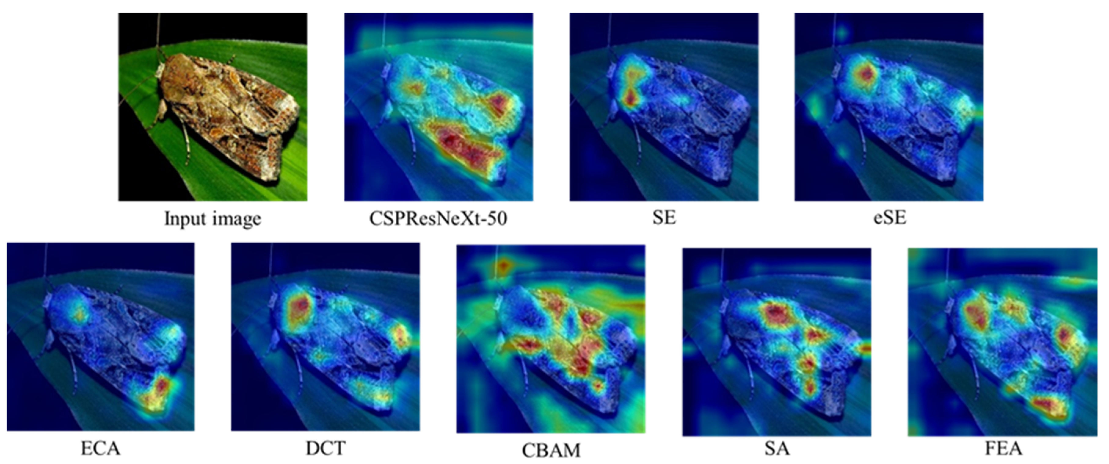
2.2. Visual Attention Mechanism

As an effective information focusing technique, the plug-and-play attention module is an effective means to improve the performance of deep learning models. The Squeeze-and-Excitation module proposed by Squeeze-and-Excitation Networks (SENet) [22] obtains global features by extracting features from the network and performing channel-level compression. Then, the global features are subjected to the excitation operation to learn the relationship between each channel and the weights of different channels, which are finally multiplied with the original feature map to obtain the final features. Since SENet uses a fully connected layer in the squeeze and excitation steps, which introduces many parameters and complex structures, some subsequent researchers have improved it. Lee et al. [44] proposed the An Energy and GPU-Computation Efficient Backbone Network for Real-Time Object Detection (VoVNet) network by replacing two fully connected layers of SENet with a two-dimensional convolution, eliminating the information loss. The hidden problem of information loss is well solved. Similarly, Wang et al. [35] proposed Efficient Channel Attention for Deep Convolutional Neural Networks (ECA-Net) after meticulous comparison experiments, replacing the fully connected layer of SENet with a one-dimensional convolution to further reduce the number of parameters. Woo et al. [45] proposed a CBAM module that combines both spatial and channel attention. From another perspective, Qin et al. [46] proved that the traditional global average pooling is a particular case of feature decomposition in the frequency domain, and proposed Frequency Channel Attention Networks (FcaNet) with multiple feature channels compared to the above approaches that only consider the relationship between channels. Zhang et al. [47] proposed a Shuffle Attention (SA) module that effectively combines spatial attention and channel attention, which first groups different channels into multiple sub-features, and then integrates each sub-module’s complementary channel and spatial attention using the shuffle units.

These attention methods have proven effective in coarse-grained recognition tasks, but are not as effective when applied to pest and disease datasets with complex backgrounds containing fine-grained problems. The fine-grained problem requires finding the most discriminative regions for each sample without losing secondary information, which often contains rich representational ability. For this reason, we propose the Feature Enhanced Attention (FEA) module, which preserves the complete image information by locating and enhancing the target features.

2.3. Fine-Grained Visual Recognition Modeling

Unlike coarse-grained image classification tasks such as object recognition, the goal of fine-grained image recognition is to correctly identify objects in hundreds and thousands of sub-classes within a large class. Objects in the same sub-class may have very different action poses, and objects in different sub-classes may have the same pose, which is a significant difficulty in recognition. The critical point of fine-grained image recognition is to find some local areas with subtle differences. How to effectively discover important local region information and obtain powerful features becomes a fundamental problem to be solved by fine-grained image recognition algorithms.

To obtain a more robust feature representation, Kong et al. [48] used two identical feature extractors to significantly reduce the computational expenditure. Li et al. [49] applied power matrix normalization to compute covariance pooling to obtain higher order features. In order to create meaningful fine-grained patterns, Du et al. [50] used a progressive strategy to achieve cross-scale feature fusion and used the idea of image chunking and then blending and stitching to construct training images. Zhang et al. [47] captured standard discriminative features by interacting feature channels in images of the same class. Similarly, Ji et al. [51] proposed an attentional convolutional binomial neural tree architecture by using the sum of nodes as the basis to enhance the judgment of recognition results. In a recent work, Gao et al. [23] used a bilinear network to mine complementary features of images and used metric learning to distinguish differences between different inputs. Zhuang et al. [20] captured the contrast differences by pairwise interaction between two images to improve the ability of identifying fine-grained differences.

Overall, these fine-grained recognition approaches have shown superior performance in modeling public large-scale data. However, there are still several vital limits of these models hindering their further applications in real-world agriculture scenarios. On the one hand, these models generally construct massive network parameters and structures to ensure model performance, which is computationally expensive and time-consuming in careful tuning procedures. On the other hand, most existing models are not only designed for real-world agricultural tasks. As a result, the reliability and uncertainty of the visual recognition are often overlooked. Currently, some studies based on the technological migration of existing deep learning models have been introduced to pest and disease identification in natural agriculture practices. For example, Lin et al. [52] proposed an M-bCNN neural network based on a convolution kernel matrix arrangement and integrated optimizations, such as DropConnect and local response normalization, to solve the recognition problem of winter wheat leaf disease; the network effectively identifies the local semantic differences with an average verification accuracy up to 96.5%.

In summary, due to the problems of complex backgrounds, occlusions, and lighting in natural environments, agricultural pest and disease recognition is a challenging fine-grained visual classification problem. Traditional deep learning methods are only suitable for period-specific static identification of a small number of pest classes on a specific crop part area; without dynamically examining temporal and environmental changes of different sample objects within the same seed class, such methods are not scientific. Moreover, the existing fine-grained methods are not applied to the field of pest identification. Thus, in this paper, we propose a novel Fe-Net model with significantly optimized strategies for fine-grained pest and disease recognition, achieving better performance than other widely used coarse-grained and fine-grained recognition models.

3. Methods and Materials

This section presents the details of our fine-grained Fe-Net approach for crop pest and disease identification, and the overall architecture is shown in Figure 2. Firstly, according to actual application requirements, we filter the existing dataset and add some sample images collected by IoT sensors and devices from the unique dataset construction. Then, to enhance the raw data scale, the sample images undergo some pre-processing steps, including rotation, HSV (a color characteristic; hue, saturation, and value) changing, Cutmix (regularization strategy to train strong classifiers with localizable features), etc. Subsequently, all images are subjected to feature extraction by an improved backbone network based on the Cross-Stage Partial network (CSP) operation. In detail, we add a spatial feature-enhanced attention module to force the network to focus on the highly representative regions while ignoring the low-response regions. Unlike general channel attentions, our attention method achieves a better spatial relationship according to the partial location of each sample. Moreover, we add a higher-order pooling module to compute the covariance matrix of the features by iterating over the square root of the matrix before feeding it into the classifier. Finally, we introduce the specific settings of the loss function and other hyper-parameters to train the entire model network more effectively.

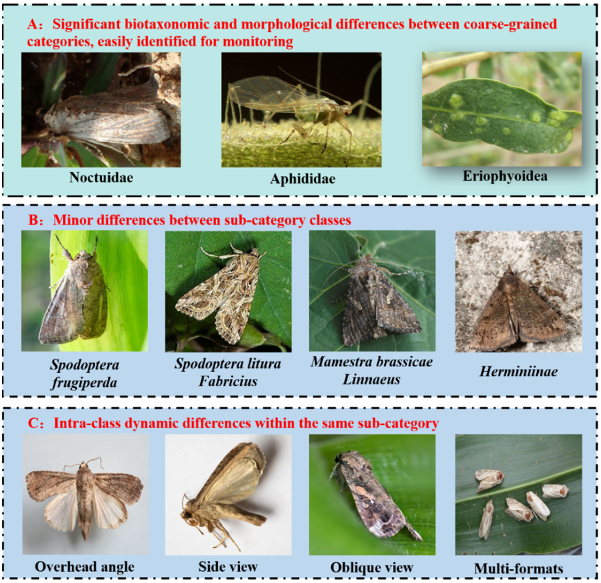
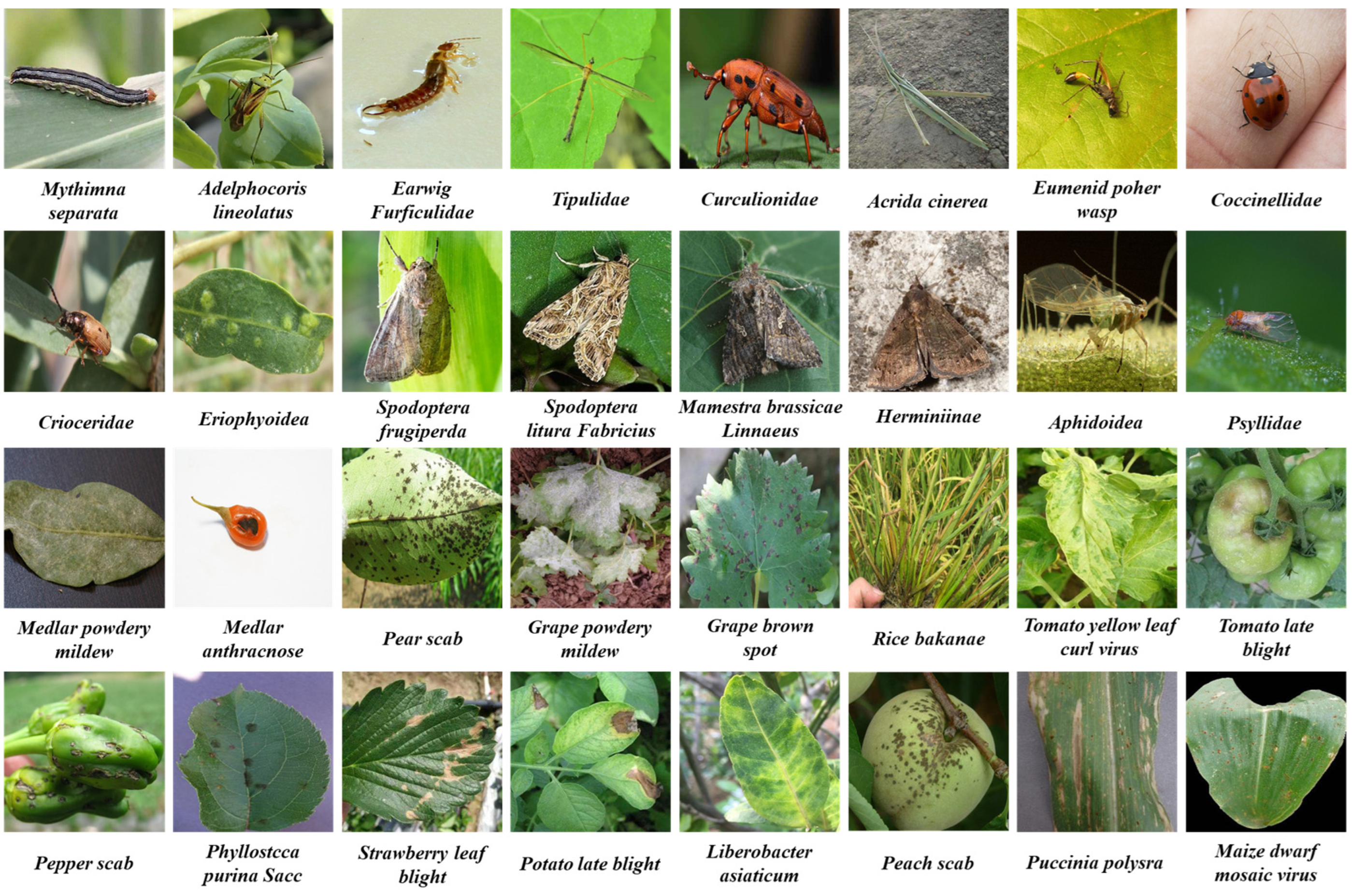
3.1. CropDP-181 Dataset

In order to guarantee the dataset scale and quality for training deep learning network architectures, we construct a new crop pest and disease dataset named CropDP-181 for identification performance in the virtual agriculture environment. All images are sourced in two ways. The first part of the dataset relies on the Internet of Things monitoring system in agricultural practices. The data collection relies on the IoT supervisory system and sensors deployed in different greenhouses and farmlands. All pest and disease image data are automatically gathered by various IOT cameras, surveillance cameras, automatic equipment, and robots, and are then transmitted to the backend cloud server through 4G/WIFI wireless channels and other wired communication channels. The image collection of these samples is carried out in time slots from July 2018 to July 2020, mainly focusing on northern regions of China such as Beijing, Shandong, Hebei, and Ningxia. In order to eliminate the impact of various data differences on the modeling process, including focal lengths, angles, aperture, equipment and camera types, data storage format, etc., we unify all image sizes to the resolution of 1000 × 1000 pixels. Then, 33,160 original images are collected by our sensors and devices. These photos have been annotated by some agronomists.

Image samples are also sourced from three public datasets: the IP102 dataset, the Inaturalist dataset, and the AIChallenger dataset. According to the actual situation, we clean some high-quality photos from these datasets into our dataset, selecting 33,801, 33,370, and 23,656 images from the IP102, Inaturalist, and AIChallenger datasets, respectively. Finally, we integrated the publicly available 90,827 images with the raw collected 33,160 images to construct the new CropDP-181 Dataset with 123,987 images in total. This dataset has a large enough number of images to train and test different intelligent models. Moreover, there are 134 pest categories and 47 disease categories, 181 in total, which host different crops, including apples, cherries, tomatoes, wheat, etc. Some data samples of different pest and disease categories are shown in Figure 3. Each category of pests and diseases contains different image samples of the onset stage, and at least 110 image samples for each category to ensure the basic data requirements for model training. This dataset contains multiple fine-grained factors—i.e., similarities in the morphology and environment of different species, and significant differences in developmental disease cycle variation, plant tissues, light, etc., of the same species—and thus can not only describe the complexity of the natural agricultural environment to some extent, but also contains challenging fine-grained pests and diseases. For more details of the data, please refer to

Table A1. CropDP-181 Dataset.

No.	Annotation Names	Image Sample Numbers	Associated Crops or Plants	Actual Collection	IP102 Dataset	Inaturalist Dataset	AIChallenger Dataset	Additional Info
1	Spodoptera exigua	214	Rice, sugar cane, corn, Compositae, cruciferous, etc.	38	65	111	0	Pests
2	Migratory locust	122	Red grass, barnyard grass, climbing grass, sorghum, wheat, etc.	40	25	57	0	Pests
3	Meadow webworm	230	Beet, soybean, sunflower, potato, medicinal materials, etc.	43	73	114	0	Pests
4	Mythimna separata	134	Wheat, rice, millet, corn, cotton, beans, etc.	44	59	31	0	Pests
5	Nilaparvata lugens	155	Rice, etc.	47	88	20	0	Pests
6	Sogatella furcifera	152	Rice, wheat, corn, sorghum, etc.	50	32	70	0	Pests
7	Cnaphalocrocis medinalis	154	Rice, barley, wheat, sugar cane, millet, etc.	51	80	23	0	Pests
8	Chilo suppressalis	156	Rice, etc.	52	45	59	0	Pests
9	Sitobion miscanthi	164	Wheat, barley, oats, naked oats, sugar cane, etc.	54	31	79	0	Pests
10	Rhopalosiphum padi	174	Wheat, barley, oats, etc.	58	91	25	0	Pests
11	Schizaphis graminum	280	Wheat, barley, oats, sorghum, rice, etc.	93	33	154	0	Pests
12	Leptinotarsadecemlineata	314	Potato, tomato, eggplant, chili, tobacco, etc.	104	43	167	0	Pests
13	Cydiapomonella	436	Apples, pears, apricots, etc.	145	112	179	0	Pests
14	Locusta migratoria manilensis	867	Wheat, rice, tobacco, fruit trees, etc.	189	395	283	0	Pests
15	Grassland caterpillar	370	Cyperaceae, Gramineae, Leguminosae, etc.	123	48	199	0	Pests
16	Sitodiplosis mosellana Géhin	470	Wheat, etc.	156	164	150	0	Pests
17	Plutella xylostella_Linnaeus	371	Cabbage, purple cabbage, broccoli, etc.	123	229	19	0	Pests
18	Trialeurodes vaporariorum	402	Cucumber, kidney bean, eggplant, tomato, green pepper, etc.	134	18	250	0	Pests
19	Bemisia tabaci_Gennadius	403	Tomato, cucumber, zucchini, cruciferous vegetables, fruit trees, etc.	134	67	202	0	Pests
20	Aphis gossypii Glover	417	Pomegranate, pepper, hibiscus, cotton, melon, etc.	139	265	13	0	Pests
21	Myzus persicae	460	Vegetables, potatoes, tobacco, stone fruit trees, etc.	153	287	20	0	Pests
22	Penthaleus major	492	Wheat, etc.	164	65	263	0	Pests
23	Petrobia latens	493	Wheat, etc.	164	43	286	0	Pests
24	Helicoverpa armigera	513	Corn, zucchini, pea, wheat, tomato, sunflower, etc.	171	271	71	0	Pests
25	Spodoptera exigua	546	Corn, cotton, sugar beet, sesame, peanut, etc.	0	187	359	0	Pests
26	Apolygus lucorum	546	Cotton, mulberry, jujube, grape, cruciferous vegetables, etc.	0	376	170	0	Pests
27	Bemisia tabaci	1255	Cucumber, tomato, eggplant, zucchini, cotton, watermelon, etc.	0	611	644	0	Pests
28	Ostrinia furnacalis	662	Corn, wheat, etc.	0	347	315	0	Pests
29	Ostrinia nubilalis	1316	Corn, sorghum, hemp, rice, sugar beet, sweet potato, etc.	0	693	623	0	Pests
30	Tetranychus turkestani	1234	Cotton, sorghum, strawberry, beans, corn, potato, etc.	0	710	524	0	Pests
31	Tetranychus truncates Ehrar	1477	Cotton, corn, polygonum, paper mulberry, etc.	0	841	636	0	Pests
32	Tetranychus dunhuangensis Wang	1288	Cotton, corn, vegetables, fruit trees, etc.	0	770	518	0	Pests
33	Yellow cutworm	1331	Wheat, vegetable, grass, etc.	0	793	538	0	Pests
34	Police-striped ground tiger	834	Rape, radish, potato, green Chinese onion, alfalfa, flax, etc.	0	241	593	0	Pests
35	Eight-character ground tiger	1237	Daisies, zinnia, chrysanthemum, etc.	0	686	551	0	Pests
36	Cotton thrips	1286	Zucchini, wax gourd, balsam pear, watermelon, tomato, etc.	0	856	430	0	Pests
37	Grass blind stinkbug	824	Cotton, alfalfa, vegetables, fruit trees, hemp, etc.	0	289	535	0	Pests
38	Alfalfa blind stinkbug	866	Cotton, mulberry, jujube, grape, alfalfa, medicinal plants, etc.	0	428	438	0	Pests
39	Green stinkbug	948	Flowers, artemisia, cruciferous vegetables, etc.	0	348	600	0	Pests
40	Tomato leaf miner	965	Tomato, potato, sweet pepper, ginseng fruit, etc.	0	496	469	0	Pests
41	Dendrolimus punctatus	1103	Masson pine, black pine, slash pine, loblolly pine, etc.	0	371	732	0	Pests
42	Japanese pine scale	1176	Pinus densiflora, pinus tabulaeformis, pinus massoniana, etc.	0	241	935	0	Pests
43	Anoplophora glabripennis	1335	Poplar, willow, wing willow, elm, sugar maple, etc.	0	497	838	0	Pests
44	American white moth	2236	Oak, phoenix tree, poplar, willow, elm, mulberry, pear, etc.	0	1620	616	0	Pests
45	Hemiberlesia matsumura	2024	Masson pine, black pine, slash pine, loblolly pine, etc.	0	1709	315	0	Pests
46	Red tip borer	1833	Masson pine, black pine, slash pine, loblolly pine, etc.	0	1497	336	0	Pests
47	Dendroctonus armandi	1824	Huashan pine, etc.	0	1275	549	0	Pests
48	Yellow bamboo locust	1527	Rigid bamboo, water bamboo, etc.	1527	0	0	0	Pests
49	Monochamus fortunei	1197	Fir, willow, etc.	1197	0	0	0	Pests
50	Sophora japonica	1498	Yang, Huai, Liu, Amorpha fruticosa, elm, maple, etc.	1498	0	0	0	Pests
51	Ulmus pumila	2228	Elm, etc.	2228	0	0	0	Pests
52	Pine geometrid	1272	Pine needles, etc.	1272	0	0	0	Pests
53	Jujube scale	1087	Acer is acacia, jujube, walnut, acacia, plum, pear, apple, etc.	1087	0	0	0	Pests
54	Coconut beetle	1109	Coconut trees, etc.	1109	0	0	0	Pests
55	Anoplophora longissima	1149	Yang, willow, birch, oak, beech, linden, elm, etc.	1149	0	0	0	Pests
56	Geometrid moth	1115	Fruit trees, tea trees, mulberry trees, cotton and pine trees, etc.	1115	0	0	0	Pests
57	Red brown weevil	405	Coconut, oil palm, brown, betel nut, mallow, date, etc.	405	0	0	0	Pests
58	Dendroctonus valens	1100	Larch, fir, pine, white pine, pine, etc.	1100	0	0	0	Pests
59	Euplophora salicina	1173	Oak, Cyclobalanopsis glauca, birch, elm, alder, park and maple, etc.	1173	0	0	0	Pests
60	Ailanthus altissima	1227	Ailanthus altissima, toona ciliata, etc.	1227	0	0	0	Pests
61	Termite	1164	Within each plant	1164	0	0	0	Pests
62	Pine wood nematode	390	Masson pine forest, etc.	390	0	0	0	Pests
63	Yellow moth	402	Jujube, walnut, persimmon, maple, apple, Yang, etc.	402	0	0	0	Pests
64	Icerya purchasi maskell	1020	Boxwood, citrus, tung, holly, pomegranate, papaya, etc.	1020	0	0	0	Pests
65	Adelphocoris lineolatus	1107	Masson pine, fir, spruce, corns, cedar, larch, etc.	1107	0	0	0	Pests
66	Tomicus piniperda	200	Huashan pine, alpine pine, Yunnan pine, etc.	200	0	0	0	Pests
67	Rice leaf caterpillar	201	Rice, sorghum, corn, sugar cane, etc.	0	91	110	0	Pests
68	Paddy stem maggot	128	Rice, etc.	0	72	56	0	Pests
69	Asiatic rice borer	814	Rice, etc.	0	560	254	0	Pests
70	Yellow rice borer	1138	Rice, etc.	0	636	502	0	Pests
71	Rice gall midge	1003	Rice, lishihe, etc.	0	813	190	0	Pests
72	Rice stemfly	124	Rice, oil grass, etc.	0	80	44	0	Pests
73	Ampelophaga	110	Grapes	0	105	5	0	Pests
74	Earwig Furficulidae	158	Rice, grasses, alismataceae, commelina, etc.	0	74	84	0	Pests
75	Rice leafhopper	223	Rice, etc.	0	64	159	0	Pests
76	Rice shell pest	763	Rice, sesame, pumpkin, cotton, etc.	0	530	233	0	Pests
77	Black cutworm	282	Corn, cotton, tobacco, etc.	0	239	43	0	Pests
78	Tipulidae	328	Cotton, corn, sorghum, tobacco, etc.	0	146	182	0	Pests
79	Yellow cutworm	150	Crops, grasses and turfgrasses	0	106	44	0	Pests
80	Red spider	282	Solanaceae, Cucurbitaceae, Leguminosae, Liliaceae, etc.	0	121	161	0	Pests
81	Peach borer	1003	Chestnut, corn, sunflower, peach, plum, hawthorn, etc.	0	401	602	0	Pests
82	Curculionidae	144	Wheat, barley, oats, rice, corn, sugar cane, grass, etc.	0	119	25	0	Pests
83	Rhopalosiphum padi	394	Plum, peach, plum, etc.	0	243	151	0	Pests
84	Wheat blossom midge	986	Wheat	0	424	562	0	Pests
85	Pentfaleusmajor	576	Wheat, barley, peas, broad beans, rape, Chinese milk vetch, etc.	0	308	268	0	Pests
86	Aphidoidea	142	Wheat, barley, peas, alfalfa, weeds, etc.	0	109	33	0	Pests
87	Spodoptera frugiperda	282	Wheat, barley, rye, oat, sunflower, dandelion, green bristlegrass, etc.	0	142	140	0	Pests
88	Spodoptera litura Fabricius	227	Wheat	0	139	88	0	Pests
89	Mamestra brassicae Linnaeus	169	Wheat, oats, barley, etc.	0	23	146	0	Pests
90	Herminiinae	2730	Wheat, rice, etc.	0	20	2710	0	Pests
91	Cabbage army worm	237	Cabbage, cabbage, radish, spinach, carrot, etc.	0	78	159	0	Pests
92	Beet spot flies	116	Beet, cabbage, rape, cabbage, etc.	0	64	52	0	Pests
93	Psyllidae	925	Pear, peach, etc.	0	552	373	0	Pests
94	Alfalfa weevil	172	Clover, etc.	0	37	135	0	Pests
95	Acrida cinerea	273	Pea, soybean, sunflower, hemp, beet, cotton, tobacco, potato	0	252	21	0	Pests
96	Legume blister beetle	130	Legume	0	21	109	0	Pests
97	Therioaphis maculata buckton	244	Leguminosae forage	0	81	163	0	Pests
98	Odontothrips loti	153	Alfalfa	0	100	53	0	Pests
99	Thrips	320	Eggplant, cucumber, kidney bean, pepper, watermelon, etc.	0	195	125	0	Pests
100	Alfalfa seed chalcid	491	Leguminosae forage seed	0	208	283	0	Pests
101	Pieris canidia	1003	Cauliflower	0	839	164	0	Pests
102	Slug caterpillar moth	190	Bamboo and rice	0	99	91	0	Pests
103	Grape phylloxera	284	Grape	0	165	119	0	Pests
104	Colomerus vitis	176	Grape	0	16	160	0	Pests
105	Oides decempunctata	1003	Grapes, wild grapes, blackberries, etc.	0	938	65	0	Pests
106	paranthrene regalis butler	260	Grape	0	190	70	0	Pests
107	Eumenid poher wasp	330	Rice, corn, sorghum and wheat, etc.	0	16	314	0	Pests
108	Coccinellidae	444	Wheat, citrus, zanthoxylum bungeanum, citrus, etc.	0	23	421	0	Pests
109	Phyllocoptes oleiverus ashmead	177	Citrus	0	109	68	0	Pests
110	Crioceridae	177	Rice, centurion, euonymus japonicus, etc.	0	70	107	0	Pests
111	Ceroplastes rubens	450	Laurel, gardenia, osmanthus, rose, etc.	0	450	0	0	Pests
112	Parlatoria zizyphus lucus	117	Citrus plants, dates, coconuts, oil palm, laurel.	0	97	20	0	Pests
113	Aleurocanthus spiniferus	192	Citrus, oil tea, pear, persimmon, grape, etc.	0	33	159	0	Pests
114	Tetradacus c bactrocera minax	194	Mandarin orange and pomelo	0	116	78	0	Pests
115	Bactrocera tsuneonis	635	Citrus	0	257	378	0	Pests
116	Phyllocnistis citrella stainton	219	Citrus, willow, kumquat, etc.	0	85	134	0	Pests
117	Aphis citricola vander goot	311	Apple, amomum villosum, begonia, etc.	0	253	58	0	Pests
118	Atractomorpha sinensis Bolivar	259	Canna, celosia, chrysanthemum, hibiscus, poaceae, etc.	0	236	23	0	Pests
119	Sternochetus frigidus Fabricius	154	Mango	0	107	47	0	Pests
120	Mango flat beak leafhopper	1003	Mango	0	244	759	0	Pests
121	Flea beetle	618	Glycyrrhrizae radix, willow seedlings, etc.	0	64	554	0	Pests
122	Brevipoalpus lewisi mcgregor	556	Parthenocissus tricuspidata, magnolia officinalis, lilac, etc.	0	390	166	0	Pests
123	Polyphagotars onemus latus	4385	Melon, eggplant, pepper, etc.	0	1118	3267	0	Pests
124	Cicadella viridis	120	Poplar, willow, ash, apple, peach, pear, etc.	0	82	38	0	Pests
125	Rhytidodera bowrinii white	210	Mango, cashew nuts, face, etc.	0	53	157	0	Pests
126	Aphis citricola Vander Goot	110	Apple, sand fruit, begonia, etc.	0	84	26	0	Pests
127	Deporaus marginatus Pascoe	296	Mango, cashew nut and almond	0	149	147	0	Pests
128	Adristyrannus	267	Citrus, apple, grape, loquat, mango, pear, peach, etc.	0	230	37	0	Pests
129	Salurnis marginella Guerr	285	Coffee, tea, camellia oleifera, citrus, etc.	0	272	13	0	Pests
130	Dacus dorsalis	201	oranges, tangerines, etc.	0	174	27	0	Pests
131	Dasineura sp	1247	lychee, etc.	0	555	692	0	Pests
132	Trialeurodes vaporariorum	1045	Cucumber, kidney bean, eggplant, tomato, green pepper, etc.	0	623	422	0	Pests
133	Eriophyoidea	361	Citrus, apple, grape, loquat, mango, pear, peach, etc.	0	0	361	0	Pests
134	Mane gall mite	854	Chinese wolfberry	0	0	854	0	Pests
135	Mulberry powdery mildew	260	White mulberry	0	0	0	260	Diseases
136	Tobacco anthracnose	229	tobacco	0	0	0	229	Diseases
137	Apple_Scab general	321	Apple	80	0	0	241	Diseases
138	Apple_Scab serious	232	Apple	58	0	0	174	Diseases
139	Apple Frogeye Spot	650	Apple	162	0	0	488	Diseases
140	Cedar Apple Rust general	277	Apple	69	0	0	208	Diseases
141	Medlar powdery mildew	170	Medlar	42	0	0	128	Diseases
142	Medlar anthracnose	170	Medlar	42	0	0	128	Diseases
143	Grape powdery mildew	290	Grape	72	0	0	218	Diseases
144	Tehon and Daniels serious	254	Corn	63	0	0	191	Diseases
145	Rice bakanae	736	Corn	184	0	0	552	Diseases
146	Puccinia polysora serious	541	Corn	135	0	0	406	Diseases
147	Puccinia polysra	316	Corn	79	0	0	237	Diseases
148	Curvularia leaf spot fungus serious	758	Corn	189	0	0	569	Diseases
149	Maize dwarf mosaic virus	1241	Corn	310	0	0	931	Diseases
150	Grape Black Rot Fungus general	580	Grape	145	0	0	435	Diseases
151	Grape Black Rot Fungus serious	704	Grape	176	0	0	528	Diseases
152	Grape Black Measles Fungus general	769	Grape	192	0	0	577	Diseases
153	Grape Black Measles Fungus serious	637	Grape	159	0	0	478	Diseases
154	Grape Leaf Blight Fungus serious	960	Grape	240	0	0	720	Diseases
155	Liberobacter asiaticum	1796	Orange	699	0	0	1097	Diseases
156	Citrus Greening June serious	1748	Orange	687	0	0	1061	Diseases
157	Grape brown spot	1305	Grape	326	0	0	979	Diseases
158	Peach_Bacterial Spot serious	1173	Peach	293	0	0	880	Diseases
159	Peach scab	695	Peach	327	0	0	368	Diseases
160	Pepper scab	512	Pepper	81	0	0	431	Diseases
161	Pear scab	519	Pear	232	0	0	287	Diseases
162	Potato_Early Blight Fungus serious	692	Potato	109	0	0	583	Diseases
163	Phyllostcca pirina Sacc	452	Potato	240	0	0	212	Diseases
164	Potato_Late Blight Fungus serious	623	Potato	113	0	0	510	Diseases
165	Strawberry_Scorch general	601	Strawberry	219	0	0	382	Diseases
166	Strawberry_Scorch serious	673	Strawberry	97	0	0	576	Diseases
167	Tomato powdery mildew general	630	Tomato	365	0	0	265	Diseases
168	Tomato powdery mildew serious	487	Tomato	83	0	0	404	Diseases
169	Strawberry leaf blight	939	Strawberry	287	0	0	652	Diseases
170	Tomato_Early Blight Fungus serious	617	Tomato	112	0	0	505	Diseases
171	Tomato_Late Blight Water Mold general	611	Tomato	302	0	0	309	Diseases
172	Tomato_Late Blight Water Mold serious	830	Tomato	163	0	0	667	Diseases
173	Tomato_Leaf Mold Fungus general	807	Tomato	371	0	0	436	Diseases
174	Tomato_Leaf Mold Fungus serious	471	Tomato	87	0	0	384	Diseases
175	Tomato_Septoria Leaf Spot Fungus general	549	Tomato	281	0	0	268	Diseases
176	Tomato_Septoria Leaf Spot Fungus serious	1132	Tomato	210	0	0	922	Diseases
177	Tomato Mite Damage general	930	Tomato	319	0	0	611	Diseases
178	Tomato Mite Damage serious	929	Tomato	480	0	0	449	Diseases
179	Tomato YLCV Virus general	1212	Tomato	616	0	0	596	Diseases
180	Tomato YLCV Virus serious	2350	Tomato	524	0	0	1826	Diseases
181	Tomato Tomv	599	Tomato	301	0	0	298	Diseases
	TOTAL	123,987		33,160	33,801	33,370	23,656

in the Appendix A.

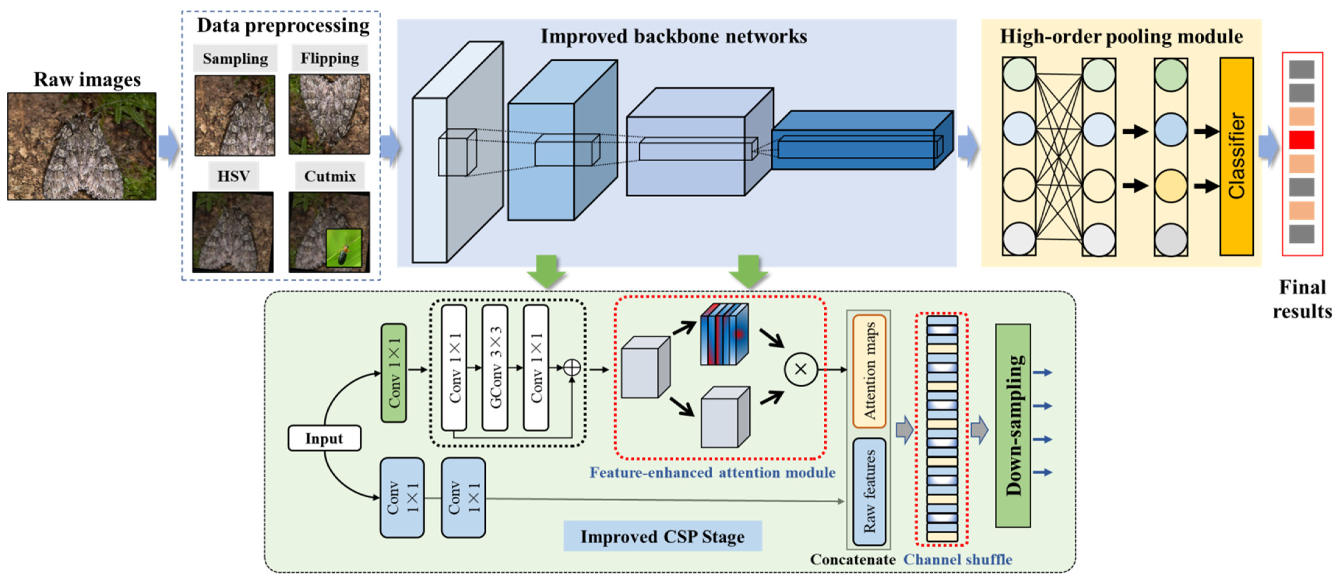
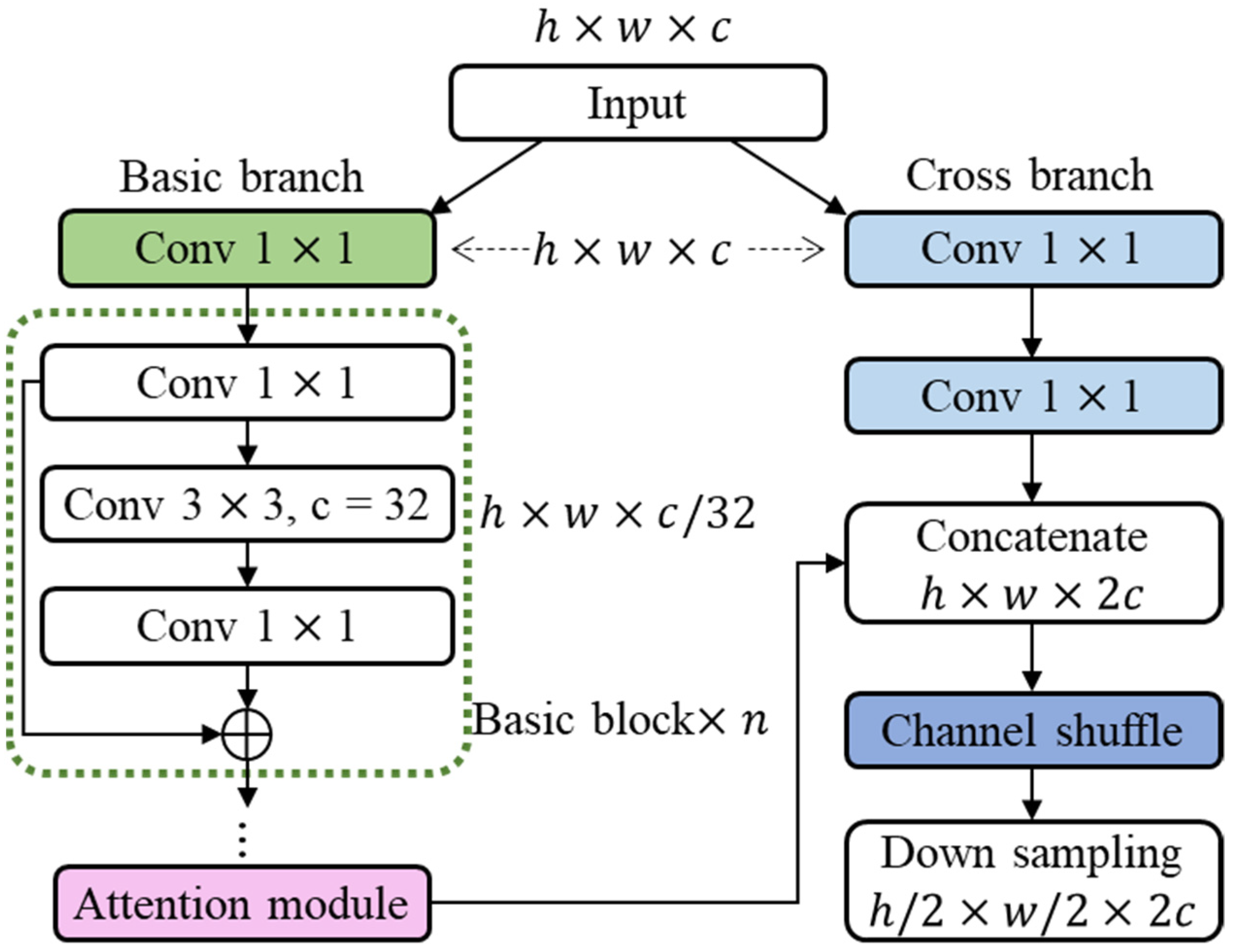
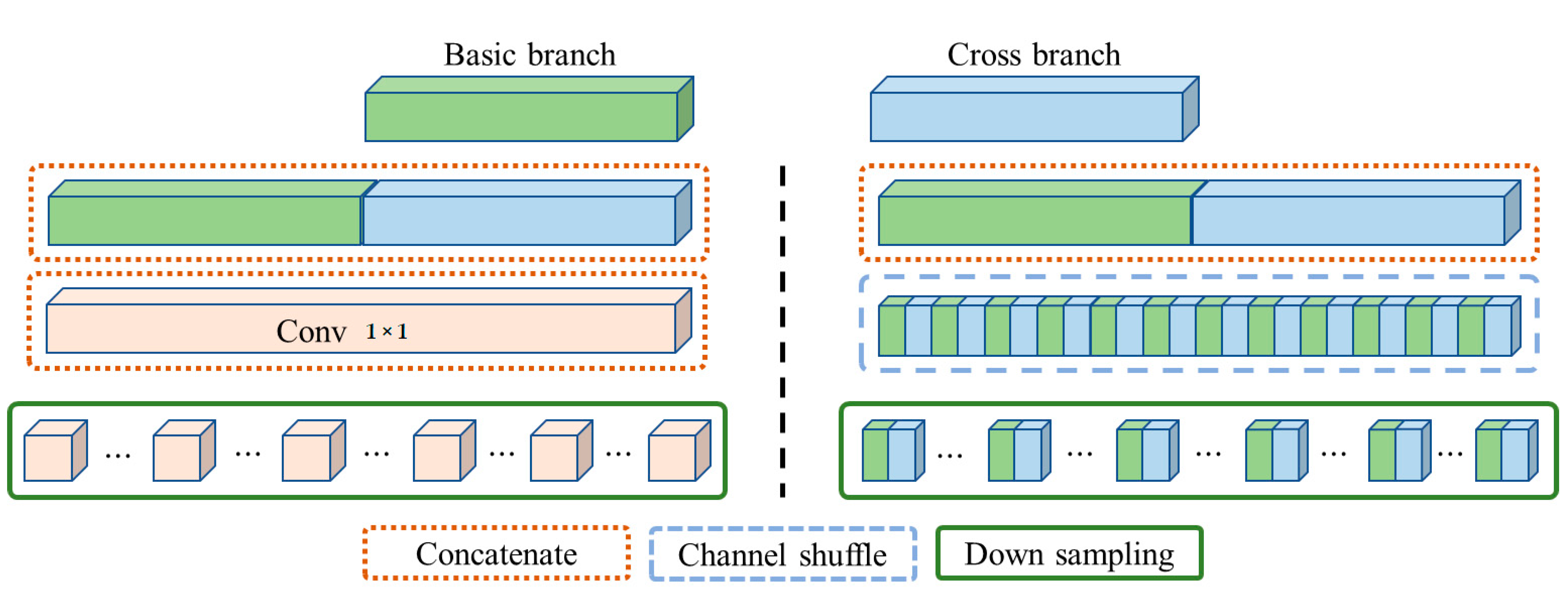
3.2. Improved CSP-Stage-Based Backbone

With its superior residual structure, ResNet has dramatically eliminated the gradient explosion and disappearance caused by overly deep networks, allowing researchers to train deeper neural networks, thus enabling recognition accuracy of downstream tasks beyond the human level. However, when the network level becomes more profound, the improvement in the number of parameters does not match the promotion in recognition accuracy. It even requires twice the number of additional parameters and computation to improve the accuracy by 1%, due to the single path of gradient information propagation in the network and, often, the existence of duplicate gradient information in the convolutional module. CSPNet [35] is a new variant network of the ResNet family, the structure of which prevents excessive repetitive gradient information by truncating the gradient flow, enhances the learning capability of CNN, eliminates computational bottlenecks, and effectively reduces memory costs. CSPNet treats feature maps with the exact resolution at each layer as a stage and adds cross-stage branches on the primary branch side, so that a portion of the features can directly skip all computational processes in that stage, which ensures network performance while reducing the number of parameters.

In this section, we take the residual block of ResNeXt [53] as the basic module and improve the stage module of CSPNet to propose CSPNet-v2. The feature extraction capability of the essential branch is enhanced by adding the spatial attention module after the primary branch. The 1 × 1 fusion convolution is removed from the original model by replacing the channel shuffle module to realize the feature interaction between the primary branch and the spanning branch, which further enhances the feature extraction ability of the proposed network. The schematic diagram of the improved CSP-stage module is shown in Figure 4.

The input $X\in {ℝ}^{h\times w\times c}$ at each stage is convolved by two 1 × 1 convolutions, in which the basic branches are convolved, and then n basic modules are added. Each primary module can be any combination of network structures, such as ResBlock, ResXBlock, DenseBlock, or some lightweight network structures, such as Ghost Bottleneck [54]. In the subsequent experiments of this paper, the basic module used is ResXBlock. After n basic modules, the features are further enhanced by the attention module. The following equation can express the computation process of the primary branch:

$$X_{Basic}=F_{att}(F_{Basic}(f_{1\times 1}(X)))$$

(1)

where $f_{1\times 1}$ denotes the 1 × 1 convolution, $F_{Basic}$ is the combination of n basic modules, and $F_{att}$ is the attention module. Subsequently, the two sets of features, essential branch and spanning branch, are stitched together to obtain $X\in {ℝ}^{h\times w\times 2c}$, and increasing the information flow between the two sets of features is achieved by channel blending.

Inspired by Shufflenet [55], a channel shuffling operation is added to contrast contextual relationships and enhance information interaction among multiple feature channels, leading to the improved CSP-stage module. We observe that the spanning branches play the role of gradient truncation. However, since group convolution is used for down-sampling, direct splicing reduces the feature extraction capability of the network, and adding channel shuffling enhances the feature interaction between the primary and spanning branches, as shown in Figure 5, and the added position is shown in Figure 4. Finally, the output $X\in {ℝ}^{h/2\times w/2\times 2c}$ of each CSP-stage is obtained after the down-sampling module, which does not play a role in the last stage in the network. The computational process of each stage can be expressed by the following equation.

$$\tilde{X}=F_{down}(S(X_{Basic},X_{Cross}))$$

(2)

where $X_{Basic}$ denotes the output of the primary basic branch, $X_{Cross}$ denotes the output of the spanning branch, $S$ denotes channel mixing, and $F_{down}$ denotes down-sampling.

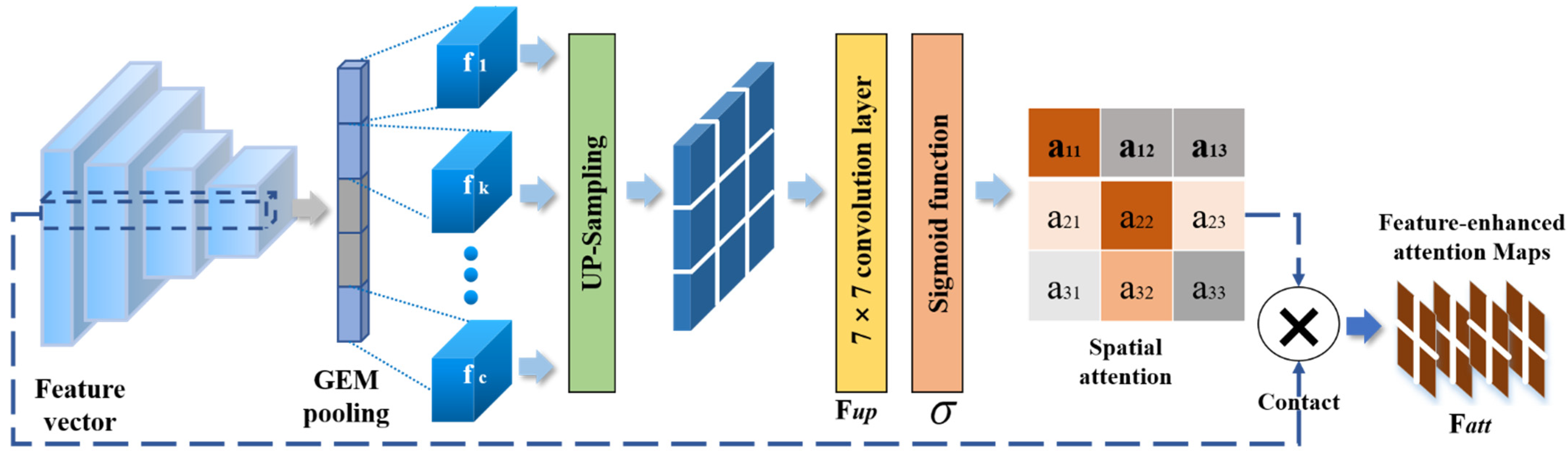
3.3. Spatial Feature-Enhanced Attention Module

To further improve the backbone network’s performance and apply it to fine-grained image classification tasks, we also propose a novel spatial feature-enhanced attention (FEA) module. Coarse-grained image classification tasks often require finding only the most discriminative part of the image to extract attention to the image. Thus, the main task of fine-grained image classification is to build powerful modules or technologies for effectively identifying large intra-class variation and small inter-class variation. However, standard attention methods only focus on the most distinguishable regions while ignoring other minor information usually contributing to the recognition results, which makes it difficult to effectively improve the performance in fine-grained image classification tasks. For fine-grained image classification tasks, attention methods should focus more on the critical information of the image in space and effectively extract regions that contain all information.

First, we down-sample the features using generalized mean pooling (GEM) [56], a pooling method widely used in the image retrieval range. GEM contains a learnable parameter P. GEM is mean pooling when p = 1, maximum pooling when p→∞, and between maximum and mean pooling when 1 < p < ∞. GEM pooling is achieved by averaging the entire feature GEM pooling averages exponentially over the whole feature map by summing each pixel of the map to the p power and then opening the p power. The specific formula of GEM is as follows.

$$f={[f_1\dots f_k\dots f_c]}^{\mathrm{T}},f_k={(\frac{1}{\left|X_i\right|}{\displaystyle \sum _{x\in X_i}{x}^p})}^{\frac{1}{p}}$$

(3)

where $X_i\in {ℝ}^{h\times w\times c}$ is the input to the pooling layer, $c$ is the number of channels, and $f\in {ℝ}^{h/2\times w/2\times c}$ is the output vector of the pooling layer. Subsequently, we up-sample $f$ to make its dimension the same as the input dimension to obtain $\tilde{f}\in {ℝ}^{h\times w}$, and perform feature extraction by convolution with a kernel size of 7 × 7, and finally go through Sigmoid to obtain the final spatial attention. The specific formula is as follows.

$$F_{att}=\sigma (Con{v}_{7\times 7}(F_{up}(f)))+X_i$$

(4)

where $F_{up}$ denotes up-sampling, $Con{v}_{7\times 7}$ denotes the 7 × 7 convolution, and $\sigma$ denotes the $Sigmoid$ activation function. The overall module schematic is shown in Figure 6.

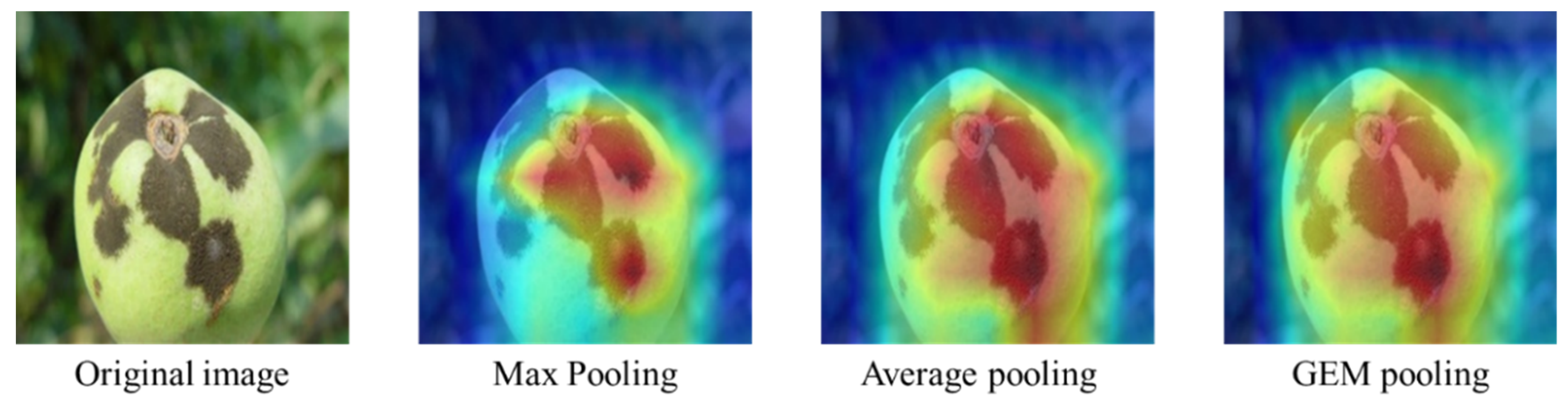
3.4. Iterative Computation of Matrix Square Root for Fast Training of Global Covariance Pooling

After the input image is extracted by the backbone network features, the features and discriminative expressions are effectively learned from low to high level, and a set of features for representing the image is obtained. Most of the works are carried out by global average pooling or maximum global pooling to reduce the dimensionality of the features, and these first-order methods are often simple, fast, and effective. However, first-order methods result in information loss, and for fine-grained image classification tasks, it is more important to extract rich features for classification. Therefore, to obtain more expressive higher-order features, we introduce the matrix power normalized covariance (MPN-COV) method to contrast the high-order pooling module. For an input image, MPN-COV produces a normalized covariance matrix as a representation, which characterizes the correlation of the feature channels and specifies the shape of the feature distribution. However, the computation of the square root of the matrix requires eigenvalue decomposition (EIG) and singular value decomposition (SVD) in performing MPN-COV, which lacks the computational support of graphics processing unit (GPU) devices and codes, leading to a prolonged training process of MPN-COV. Therefore, we propose the iterative computation of matrix square root for fast training of global covariance pooling method (iSQRT-COV), which uses an iterative matrix square root algorithm for fast end-to-end training of global covariance matrix pooling. Since this method only includes matrix multiplication, it is ideal for GPUs with high parallelism capability to perform the computation, and the training process is significantly faster than MPN-COV.

The core of the optimized module has an iterative loop that first reduces the dimensionality of the input feature F to obtain $X\in {ℝ}^{w\times h\times c}$. This set of tensors is adjusted to the feature matrix $X\in {ℝ}^{n\times c},n=w\times h$. Subsequently, the covariance matrix is calculated for this feature by the following equation.

$$\Pi =X\overline{I}{X}^T$$

(5)

where $\overline{I}=\frac{1}{n}\left(I-\frac{1}{n}1\right)$; I and 1 are the unit matrix and the all-1 matrix with dimension 1 × 1, respectively. This covariance matrix is subsequently regularized to enable global convergence, using the trace of the covariance matrix $\Pi$ to regularize the matrix with the following equation.

$$P=\frac{1}{tr\left(\Pi \right)}\Pi$$

(6)

where $tr()$ denotes the trace of the matrix. After regularization, iSQRT-COV computes the square root of the matrix P using an iterative method, which is calculated as follows.

$$\begin{gathered} M_i=\frac{1}{2}{M}_{i-1}\left(3I-N_{i-1}{M}_{i-1}\right) \\ {N}_i=\frac{1}{2}\left(3I-N_{i-1}{M}_{i-1}\right)N_{i-1} \end{gathered}$$

(7)

where $M$ is the square root of the solution; $M_0=P$ and $N_0=I$; $i=1,\cdots ,k$; and $k$ denotes the number of iterations. Since the above equation involves only matrix products, it is well suited for parallel training on GPUs and requires only a few iterations to obtain an approximate solution. Since the regularization of the initial step reduces the amount of data in the network, to prevent adverse effects, the square root result is positively compensated after the iteration.

$$Out=\sqrt{tr\left(\Pi \right)}{M}_k$$

(8)

The overall steps of the high-order pooling module are shown in Algorithm 1.

Algorithm 1. The overall calculating steps of the high-order pooling module.

Calculating processes in high-order pooling module

Input:F is a feature of the input, k is the number of iterations

Output:Out is the higher-order feature of the output

$X=conv\left(F\right)$ where $X\in {ℝ}^{n\times c},n=w\times h$

$\Pi =X\overline{I}{X}^T$ where $\overline{I}=\frac{1}{n}\left(I-\frac{1}{n}1\right)$

$P=\frac{1}{tr\left(\Pi \right)}\Pi$, and set $M_0=P$, $N_0=I$

$for i to k do$ $M_i=\frac{1}{2}{M}_{i-1}\left(3I-N_{i-1}{M}_{i-1}\right)$

$N_i=\frac{1}{2}\left(3I-N_{i-1}{M}_{i-1}\right)N_{i-1}$

$Out=\sqrt{tr\left(\Pi \right)}{M}_k$

Return Out

Since re-scaling the similarity scores under supervision is a common practice in modern classification losses, we optimize the general cross-entropy loss function as following loss function during Fe-Net training and testing. We apply the label smoothing technique to modify the loss function by using the new smoothed labels to replace the original ones. The novel loss expression in this paper is as follows:

$$y^{\prime }=\left(1-\epsilon \right)\tilde{y}+\epsilon u$$

(9)

where $\tilde{y}$ is the sample label after the data processing step, $\epsilon$ is the smoothing factor, and $u$ is a fraction of the category numbers. Label smoothing drives the classification probability results of the SoftMax activation function output closer to the correct classification, and ultimately enables the network to have better generalization by suppressing the positive and negative sample output differences. Moreover, the smoothing factor is natural when the model only penalizes classification error if a prediction score is present of a sample belonging to a certain class. It thus removes the constraint of equal re-scaling and allows more flexible optimization, making it more suitable to the fine-grained classification problem.

3.5. Data Processing and Parameter Settings

There is a data imbalance in the number of image samples due to the different occurrence of diseases and insect pests and the limitation of sample collection time and location. To avoid over-fitting of the model, we enhance the data with some image pre-processing steps to expand the dataset. Those enhanced operations can artificially simulate the influence of various experimental process disturbances and environmental background changes, which will increase the generalization ability of the model during the training and testing processes. This section describes some of the settings we use in the network training process, including data processing and parameter settings.

3.5.1. Data Preprocessing

Due to the inherent characteristics of large intra-class variation and high inter-class similarity in fine-grained image classification tasks, the network is highly susceptible to overfitting during training. To avoid this situation, we performed some data pre-processing operations to enlarge the dataset.

(1) Uniformly adjusting all images to (512, 512) and randomly sampling them according to (448, 448) to exclude the interference of background factors.

(2) Flipping all images horizontally and vertically with a probability of 0.3 to increase the diversity of the images, and randomly rotating all images by 30°, 60°, and 90° with a probability of 0.3 to increase the adaptability of the images.

(3) Randomly varying the saturation of the images to 50% to 150% of the original image and varying the brightness to 30% to 170% of the original image in the HSV color space of the image, keeping the hue and contrast constant, to increase the light intensity variation and enhance the adaptability of the image.

(4) Regularizing the input data on the basis of the Cutmix enhancement method. Cutmix crops off a part of the region (over 0 pixels) to randomly fill the region pixel values of other training data in a particular proportion. Cutmix has some advantages in improving classification results, such as preventing non-informative pixels from appearing in the training process, improving the training efficiency, and enhancing the spatial relationship. The computational process of Cutmix is shown as follows.

$$\begin{array}{c}\tilde{x}=M\odot x_a+\left(1-M\right)\odot x_b\hfill \\ \tilde{y}=\lambda y_a+\left(1-\lambda \right)y_b\hfill \end{array}$$

(10)

where $M\in {\{0,1\}}^{w\times h}$ is the binary mask to achieve crop and fill, $\odot$ is the pixel-by-pixel multiplication, and $\lambda ~Beta\left(a,a\right)$ is used to generate the crop region, and a is uniformly set to 1 in the experiments of this paper

The above steps can obtain the generalization of the network architecture and improve the robustness capability by the enhanced data, and all the images are randomly put into the network for training after the above preprocessing.

3.5.2. Parameter Settings

In the training process, we optimize the parameters of the entire network using the Ranger optimizer, which is the development variant of the Radam optimizer with the addition of a lookahead operation. On one hand, the Radam optimizer is a modification of the Adam optimization algorithm that dynamically turns on or off the adaptive learning rate based on the potential scatter of the variance, providing a dynamic warm-up without the need for adjustable parameters. On the other hand, the lookahead operation can be seen as an external attachment to the optimizer by saving two sets of weights, fast and slow weights. When the fast weights are updated k times, the slow weights are then updated one step in the direction of the current fast weights. This approach can effectively reduce the variance and achieve faster convergence.

For initialing the optimizer parameters, we use the default settings with the initial learning rate set to 1e-3 and k set to 6. The rest of the network parameters are initialized by loading the pre-training weights of CSPNet pre-trained on ImageNet (with 77.9% of Top-1 accuracy). In the whole training process, our batch size is set to 112, the overall training period is set to 100 cycles, and we use the cosine annealing learning rate reduction algorithm with restart. First, the learning rate is trained for 30 cycles at 1 × 10⁻³. The cosine annealing learning rate reduction is started at the 31st cycle, and the minimum learning rate is set to 1 × 10⁻⁶. For each restart, the learning rate is 70% of the initial learning rate of the previous cycle, and the cosine annealing learning rate is set to 1 × 10⁻⁶. Finally, the cosine annealing step is set to 2, the length base cycle of each stage is 10, and the learning rate is restarted at the 41st and 61st cycles.

4. Experimental Results

To ensure the reliability of the training, we randomly selected 15% of the 181 classes of samples as the test and validation sets (18,666 in total) and the remaining 85% as the training set (105,771 in total). We built a cloud server platform with Ubuntu 20.04LTS, which consists of a dual-core Intel Xeon E5-2690 V3@2.6 GHz × 48 processors, 128 G RAM and 2 × 2T SSD, 7 NVIDIA Tesla p40 GPUs for graphics, and 168 G computational cache. All the codes and experiments are based on the deep learning framework Pytorch 1.7.1 and TensorFlow2.4.0 under the Python 3.8.2 programming environment.

In order to evaluate the classification performance, the evaluation metrics in this paper include the following sets: Top-1 classification accuracy (Top-1 Acc), Top-5 classification accuracy (Top-5 Acc), F1-score (F₁), and average recognition time (ART).

$$Top-1Acc=\frac{TP+TN}{TP+TN+FP+FN}$$

(11)

$$Top-5Acc=\frac{T{P}_5+T{N}_5}{N}$$

(12)

$$F_1=\frac{2\times Per\times Rec}{Per+Rec}$$

(13)

$$ART=\frac{{{\displaystyle \sum }}_{i=1}^{N}time\left(i\right)}{N}$$

(14)

where True positive (TP) indicates that the predicted and actual values are all positive for a category or n categories, and True negative (TN) indicates that the predicted and actual values are negative for a category or n categories. False positive (FP) indicates that the predicted value is positive, but the actual forecast is negative, and False negative (FN) indicates that the predicted value is negative, but the actual value is positive. Those basic definitions can be combined into evaluation indicators Top-1 Acc and Top-5 Acc, which are used to evaluate the model’s prediction results for the greatest probability category and the five best categories, respectively. Similarly, precision (Per) and recall (Rec) are also calculated based on the above four definitions, which are integrated together to obtain a new judgment standard F₁. It is the harmonic average of precision and recall to comprehensively characterize the modeling classification performance, of which the minimum and maximum values are 0 and 1. Moreover, the average recognition time (ART) represents how long the trained model needs to handle a single image and recognize massive different samples in the testing stage. Obviously, the smaller the ART value, the better the efficiency modeling performance in recognizing a single image for agriculture practices.

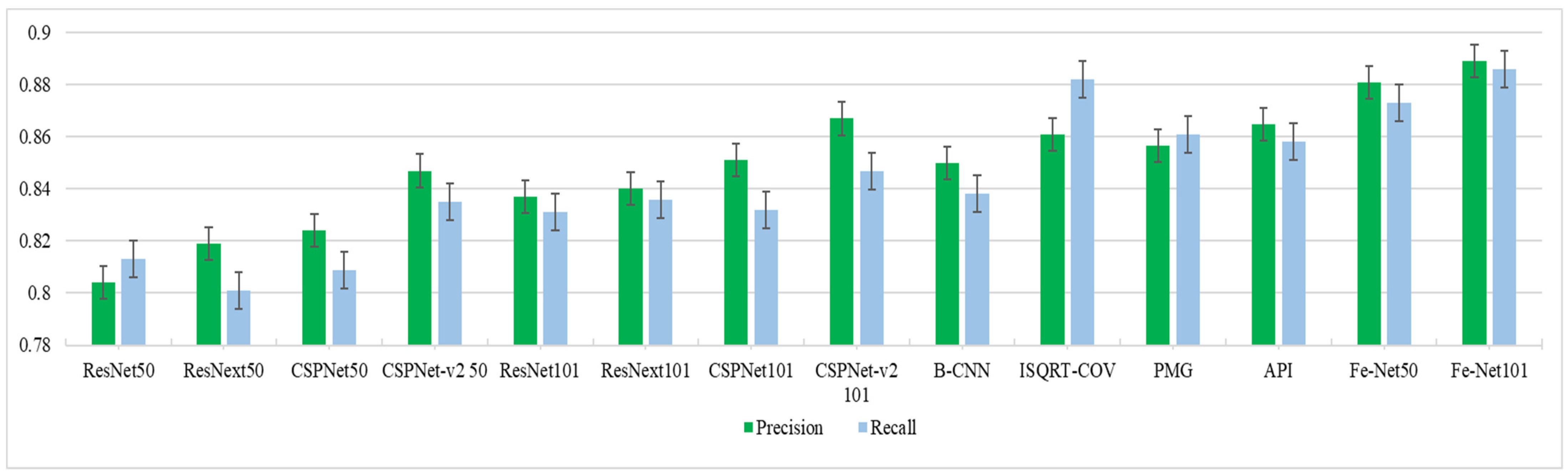
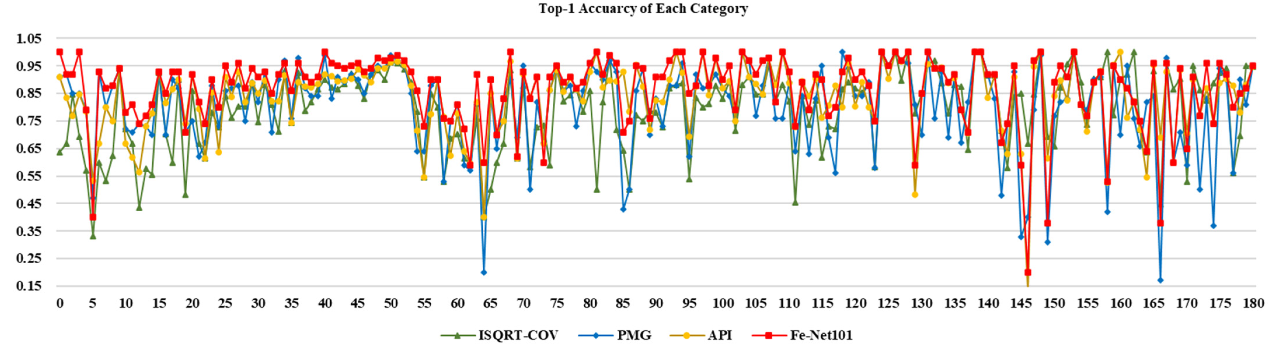
4.1. Contrastive Results

To validate the overall performance of the proposed method, we conducted a comprehensive comparison with some coarse-grained methods and fine-grained open-source methods on the proposed CropDP-181 Dataset, and the obtained results are shown in

Table 1. Comparison experimental results on CropDP-181 Dataset.

Method	Backbone	Top-1 Acc (%)	Top-5 Acc (%)	F1	ART (ms)
	VGG-16 [19]	74.62	88.87	0.794	39
	ResNet-50 [30]	76.91	90.04	0.808	34
	ResNeXt-50 [57]	77.47	90.11	0.810	33
	CSPResNeXt-50 [35]	77.86	90.18	0.816	31
	DenseNet-121 [23]	76.84	90.02	0.808	36
	CSPNet-v2-50 [35]	80.44	91.47	0.841	39
	VGG-19 [19]	76.16	89.65	0.801	59
	ResNet-101 [30]	79.19	90.53	0.834	48
	ResNeXt-101 [57]	79.81	90.76	0.838	46
	CSPResNeXt-101 [35]	80.12	91.17	0.841	43
	DenseNet-201 [23]	78.57	90.51	0.831	54
	CSPNet-v2-101 [35]	82.05	92.77	0.857	55
B-CNN [40]	VGG-19 [19]	80.38	91.57	0.844	69
iSQ-RTCOV(32k) [58]	ResNet-101 [30]	83.11	93.95	0.871	61
PMG [50]	ResNet-50	82.84	93.64	0.859	72
API-Net [20]	ResNet-50	82.67	93.87	0.861	84
Proposed Fe-Net	CSPNet-v2(50)	84.59	94.41	0.877	57
Proposed Fe-Net	CSPNet-v2(101)	85.29	95.07	0.887	61

. The CSPResNeXt-101 network is obtained by modifying it on top of ResNeXt-101 in the same way as the improvement from ResNeXt-50 to CSPResNeXt-50.

From the above table, we can see that the CSPNet method has improved the single sheet recognition time and accuracy compared with the original method in the coarse-grained network of the same scale: CSPResnext-50 has 2 ms faster single sheet recognition time and 0.39% higher accuracy compared with ResNeXt-50, while CSPResNeXt-101 has 0.39% faster recognition time compared with ResNeXt-101. Compared with ResNeXt-101, the single sheet recognition time of CSPResNeXt-101 is 3 ms faster, and the accuracy is improved by 0.31%, which verifies the effectiveness of the CSPNet method. Moreover, the recognition accuracies of the fine-grained methods are all higher than those of the coarse-grained models. For example, the iSQRT-COV (32k) network improves by 3.92% over ResNet-101.

In contrast, our proposed Fe-Net obtained the best performance, with Top-1 Acc reaching 85.29% (an improvement of 5.17%), Top-5 Acc reaching 95.08% (an improvement of 3.91%), and an F1-score of 0.887 (an improvement of 0.046) compared with CSPResNeXt-101, proving the effectiveness of the method in this paper. Although this method’s average single recognition time is only slightly improved from 43 ms to 61 ms, which is better than other fine-grained models based on complicated ResNet framework, it still meets the demand of real time. The above index results and visual heat map prove that the method proposed in this paper can solve the problem of fine-grained pest and disease image recognition and meet the requirements of practical application deployment. In Figure 7, we show the feature map visualization of different methods in different pest and disease samples, further demonstrating the scientific nature of the method in this paper.

To further demonstrate the effectiveness of the proposed method, we show a graph comparing the precision rate and recall rate of 14 methods in Figure 8. From the figure, the proposed Fe-Net101 in this paper has the best precision and recall rates of 0.889 and 0.886, respectively, while ResNet in the illustration has the lowest precision and recall rates of 0.804 and 0.813, respectively. In the coarse-grained model, the values of CSPNet-v2 in the 50-layer network are 0.847 and 0.832, respectively, while the values of CSPNet-v2 in the 101-layer network are 0.867 and 0.847, respectively, which are the best results in both levels of the network. The best precision rate of 0.865 was obtained for API in the fine-grained approach, while the best recall rate of 0.882 was obtained for ISQRT-COV. When using CSPNet-v2 as the backbone network, the precision and recall rates of ISQRT-COV improved by 3.25% and 0.4%, respectively, compared to the original ResNet101, which proves the effectiveness of the proposed network in this paper. Compared with CSPNet-v2 101, the precision and recall rates improved by 2.5% and 4.6%, respectively, after adding ISQRT-COV covariance pooling, which also proves the rationality of choosing ISQRT-COV as the higher-order feature mining method in this paper. At the top of the bar chart, we added a range line representing the standard deviations of precision and recall indicators, calculated by statistically analyzing the different results of each category in the entire dataset; the center position is determined according to the mean value, and the upper and lower limits are determined by the maximum and minimum values. Since some decimals will be ignored or rounded when calculating the index, this will lead to some deviation in the result. Therefore, we use the range line to make it more reasonable to analyze the comparison results of different models. From this analysis, the deviation range of two indicators offered by the proposed Fe-Net101 is relatively small, which means that the classification results of this model are more stable in different categories, with better effects on robustness and anti-interference ability.

4.2. Ablation Analyses

In this section, we develop some ablation comparison experiments to demonstrate the effectiveness of the proposed method.

Table 2. Ablation experiment of Fe-Net.

Method	Top-1 Acc (%)
CSPResNeXt-50	77.86
CSPResNeXt-50 + channel shuffle	78.39 (+0.53)
CSPResNeXt-50 + FEA	79.81 (+1.95)
CSPResNeXt-50 + ISQRT-COV	82.11 (+4.25)
CSPResNeXt-50 + channel shuffle + FEA + ISQRT-COV (Fe-Net)	84.59 (+6.73)

shows the comparative ablation experiments for the proposed Fe-Net. Adding channel shuffle to CSPResNeXt-50 can improve the accuracy by 0.53% without affecting any computational process. The down-sampling step uses group convolution. After the spanning branch is spliced with the primary branch, if it goes directly to down-sampling, it will form two information paths of the spanning branch, and the primary branch cannot interact appropriately. After the splicing, the features are rearranged by adding a channel shuffle, and the convolution in each group contains the information of both paths in the down-sampling step, thus increasing the information interaction between the two information paths.

The FEA is our proposed attention component for enhancing spatial information in images, which down-samples the features by GEM pooling, extracts the critical information in space, and up-samples the sampled features to the original dimension after summing and averaging, finally realizing spatial attention-based feature enhancement. To illustrate the improvement effect of the proposed FEA module on the accuracy rate, we designed comparative experiments of different attention modules based on the same basic backbone network in the form of control variables, as shown in

Table 3. Performance comparison of different attention methods on the CropDP-181 Dataset.

Method	Top-1 Acc (%)
CSPResNeXt-50	77.86
+ SE [22]	78.63 (+0.77)
+ eSE [44]	79.07 (+1.21)
+ ECA [47]	79.14 (+1.28)
+ DCT [45]	79.21 (+1.35)
+ CBAM [59]	79.19 (+1.33)
+ SA [53]	79.43 (+1.57)
+ FEA(our)	79.81 (+1.95)

.

Table 3 shows that the SE, eSE, ECA, and DCT methods are all channel attention, and these methods do not significantly improve the fine-grained pest identification problem. The brackets after each result are filled with the accuracy improvement value compared to the base model. As shown, the SE module brings only 0.77% improvement. However, the two fully connected layers in the SE module bring many extra parameters and are prone to information loss during squeezing and excitation. eSE and ECA improved the SE module by replacing the two fully connected layers with two-dimensional convolution and one-dimensional convolution, respectively, bringing a performance improvement of 1.21% and 1.28%, respectively. DCT, on the other hand, does not modify the squeezing and excitation in the SE module but generalizes the global average pooling to the frequency domain to achieve channel attention, bringing a performance improvement of 1.35%. CBAM combines spatial and channel attention and brings the best result of 1.33%, while the SA module brings a performance improvement of 1.57%. Our proposed FEA attention achieves the best performance improvement of 1.95%. We visualize the attention plots of the above methods for easy visualization of the different effects of different methods, as shown in Figure 9.

From the above Figure 9, we can observe that the coarse-grained network prefers to mine all the features of the image, and there are often influencing factors in these features that affect the performance of the network. In contrast to the coarse-grained network, the SE module can extract the central part of the features, but too much information is lost due to squeezing and excitation. Moreover, we can see that the focus of the SE method is limited to the head and ignores the features in other parts. eSE, ECA, and DCT have different focus tendencies for on each of the three methods. eSE had the head region activated by the focus and the tail was slightly activated, ECA had the tail region activated focally while the head was activated secondarily, and DCT activated both the head and the tail region. As shown, CBAM and SA yielded more activated regions than these pure channel attentions. However, the performance was slightly degraded because CBAM also activated some background factors. The SA method achieved good results with the head as along with the body being activated. Our proposed FEA module has a slightly different focus from the SA method, focusing on the head and tail information, and the focus areas of the FEA are at the boundary between the sample and the background, separating the foreground and the background.

Moreover, we visualize the activation state when no pooling method is applied to the features, as shown in Figure 10. The maximum pooling extracts the maximum response in the range, which can extract important local features; the average pooling extracts the average response in the range, which can obtain richer global features. The larger the value, the more the network focuses on local features, i.e., it is closer to the maximum pooling. When the value is between 1 and infinity, the GEM pooling extracts both important local features and information-rich global features. In our experiments, we set the p value to 3.

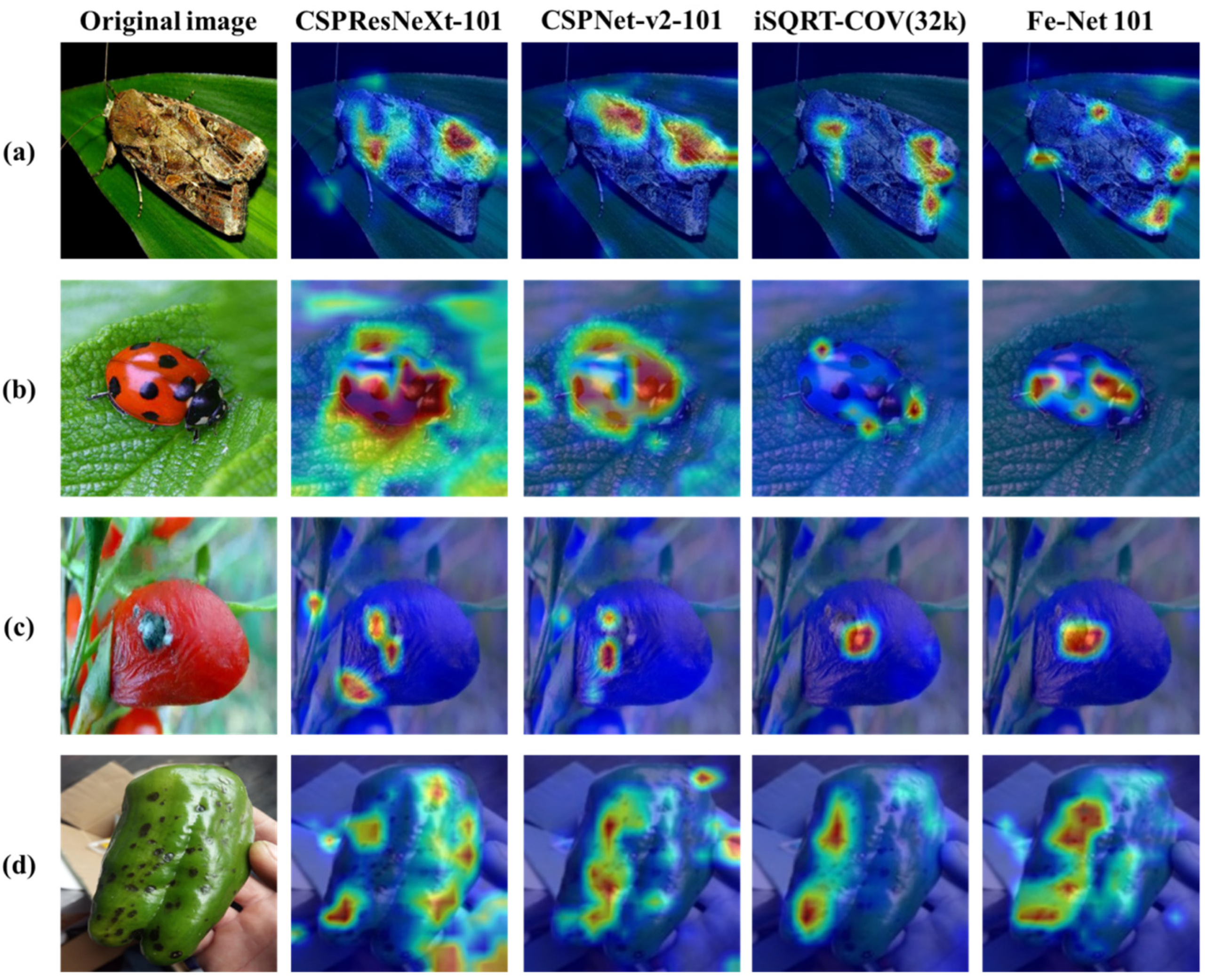
4.3. Module Effect Discussion

In order to illustrate the role of the fusion module, we carried out a visual comparison experiment by comparing the proposed method with ISQRT-COV [60], PMG [61], and API [58]. We analyzed the accuracy of each model for each type of image in the dataset, as shown in Figure 11. It can be observed that the Top-1 Acc of our method is above 80% for most of the samples, and some of the categories even reach 100% for pest and disease identification. As can be seen from Figure 11, our results are superior to the other three methods overall. Specifically, with the help of designed attention and high-order pooling modules, Fe-Net can effectively integrate multi-dimensional features extracted by different modules and eliminate redundant information among various complements, thereby improving the recognition accuracy for each type of pest image. For example, ISQRT-COV has an accuracy of 63.6% in category 0 and 69.2% in category 3; API has an accuracy of 90.9% in category 0 and 84.6% in category 3. More obviously, the ISQRT-COV has an accuracy of 41.2%, the API has an accuracy of 39.8%, and the PMG has an accuracy of 21.4% in category 64, but the accuracy of Fe-Net is 61.6, which is obviously superior to the other methods. After the gated fusing operation, the average accuracy of the Fe-Net method in this 0th pest class is up to 100%; the accuracy in the 3rd category is 100%. The fused module gradually reduces the identification difference in diverse individual modules or methods for fine-grained targets, thereby improving the overall accuracy.

However, our model still has some limitations. In two other categories, category 64 (the biological name is Icerya purchasi maskell) and category 146 (the biological name is Puccinia polysora serious), the model only achieved 45.2% and 13.3% accuracy, respectively. This shows that although the Fe-Net has dramatically improved the performance of the underlying network, it is still difficult to improve the performance for some problematic categories such as complex image backgrounds and too many poses, and it also reflects to some extent the problem of poor robustness of a single model in pest identification tasks. It is necessary to consider using better performance underlying networks or fine-grained methods to achieve further performance improvement. In future work, the model structure will be optimized to improve the identification performance. The coupling of pest and disease data will be investigated to expand the application scope of the proposed model in a smart greenhouse and farmlands, and they can be applied to other fields such as temporal prediction, signal modeling, and control systems [62,63,64,65,66,67,68,69].

5. Conclusions

In precision agriculture applications, pest and disease recognition is a typical fine-grained visual classification problem, which is still challenging to current deep learning models and other fine-grained methods. To address this critical issue, we firstly constructed a fine-grained agriculture pest and disease dataset (Crop-DP181) containing over 122,000 samples of 181 categories. Based on data pre-processing and pre-training, we proposed a feature-enhanced attention neural network (Fe-Net) to identify fine-grained crop pests and diseases in natural agriculture scenarios. The proposed Fe-Net consists of three important modules: the improved CSP-stage backbone network, the spatial FEA module, and the higher-order pooling module. Firstly, the Fe-Net applies the branch structure modification and the channel shuffling operation to establish an improved CSP-stage backbone network, which offers massive local and global features in rich perceptual dimensions. Then, a spatial feature-enhanced attention module is proposed to exploit the spatial interrelationship between different semantic regions. The high-order pooling module relying on elements of a covariance matrix computation is added to learn a more representative spatial correlation. After a series of comparison experiments on the CropDP-181 Dataset, the proposed Fe-Net achieved Top-1 Acc up to 85.29% and Top-5 Acc up to 95.07%, outperforming comparative methods. Moreover, 0.887 F₁ with only a 61 ms average recognition time demonstrates the better efficiency and robustness of Fe-Net, which meets the practical demands of different IoT devices and equipment in precision agriculture applications. The proposed approaches in the paper can combine other parameter estimation algorithms [70,71,72,73,74,75] to study the parameter identification problems of linear and nonlinear systems with different disturbances [76,77,78,79,80,81], and can be applied to other fields [82,83,84,85,86] such as signal processing and engineering application systems.

References

1. Manavalan, R. Automatic identification of diseases in grains crops through computational approaches: A review. Comput. Electron. Agric. 2020, 178, 105802. [Google Scholar] [CrossRef]
2. Kong, J.; Wang, H.; Wang, X.; Jin, X.; Fang, X.; Lin, S. Multi-stream hybrid architecture based on cross-level fusion strategy for fine-grained crop species recognition in precision agriculture. Comput. Electron. Agric. 2021, 185, 106134. [Google Scholar] [CrossRef]
3. Zheng, Y.-Y.; Kong, J.-L.; Jin, X.-B.; Wang, X.-Y.; Su, T.-L.; Zuo, M. Crop Deep: The crop vision dataset for deep-learning-based classification and detection in precision agriculture. Sensors 2019, 19, 1058. [Google Scholar] [CrossRef] [Green Version]
4. Marcu, I.M.; Suciu, G.; Balaceanu, C.M.; Banaru, A. IOT based system for smart agriculture. In Proceedings of the 11th International Conference on Electronics, Computers and Artificial Intelligence, Pitesti, Romania, 27–29 June 2019; pp. 1–4. [Google Scholar]
5. Jin, X.-B.; Zheng, W.-Z.; Kong, J.-L.; Wang, X.-Y.; Bai, Y.-T.; Su, T.-L.; Lin, S. Deep-Learning Forecasting Method for Electric Power Load via Attention-Based Encoder-Decoder with Bayesian Optimization. Energies 2021, 14, 1596. [Google Scholar] [CrossRef]
6. Ding, F.; Chen, T. Combined parameter and output estimation of dual-rate systems using an auxiliary model. Automatica 2004, 40, 1739–1748. [Google Scholar] [CrossRef]
7. Ding, F.; Chen, T. Parameter estimation of dual-rate stochastic systems by using an output error method. IEEE Trans. Autom. Control 2005, 50, 1436–1441. [Google Scholar] [CrossRef]
8. Ding, F.; Shi, Y.; Chen, T. Auxiliary model-based least-squares identification methods for Hammerstein output-error systems. Syst. Control Lett. 2007, 56, 373–380. [Google Scholar] [CrossRef]
9. Xu, L. Separable multi-innovation Newton iterative modeling algorithm for multi-frequency signals based on the sliding measurement window. Circuits Syst. Signal Process. 2022, 41, 805–830. [Google Scholar] [CrossRef]
10. Xu, L. Separable Newton recursive estimation method through system responses based on dynamically discrete measurements with increasing data length. Int. J. Control Autom. Syst. 2022, 20, 432–443. [Google Scholar] [CrossRef]
11. Zhou, Y.H.; Ding, F. Modeling nonlinear processes using the radial basis function-based state-dependent autoregressive models. IEEE Signal Process. Lett. 2020, 27, 1600–1604. [Google Scholar] [CrossRef]
12. Zhou, Y.H.; Zhang, X. Partially-coupled nonlinear parameter optimization algorithm for a class of multivariate hybrid models. Appl. Math. Comput. 2022, 414, 126663. [Google Scholar] [CrossRef]
13. Zhou, Y.H.; Zhang, X. Hierarchical estimation approach for RBF-AR models with regression weights based on the increasing data length. IEEE Trans. Circuits Syst. II Express Briefs 2021, 68, 3597–3601. [Google Scholar] [CrossRef]
14. Zhang, X. Optimal adaptive filtering algorithm by using the fractional-order derivative. IEEE Signal Process. Lett. 2022, 29, 399–403. [Google Scholar] [CrossRef]
15. Ding, J.; Liu, X.P.; Liu, G. Hierarchical least squares identification for linear SISO systems with dual-rate sampled-data. IEEE Trans. Autom. Control 2011, 56, 2677–2683. [Google Scholar] [CrossRef]
16. Ding, F.; Liu, Y.J.; Bao, B. Gradient based and least squares based iterative estimation algorithms for multi-input multi-output systems. Proc. Inst. Mech. Eng. Part I J. Syst. Control Eng. 2012, 226, 43–55. [Google Scholar] [CrossRef]
17. Xu, L.; Chen, F.Y.; Hayat, T. Hierarchical recursive signal modeling for multi-frequency signals based on discrete measured data. Int. J. Adapt. Control Signal Process. 2021, 35, 676–693. [Google Scholar] [CrossRef]
18. Kumar, S.A.; Ilango, P. The impact of wireless sensor network in the field of precision agriculture: A review. Wirel. Pers. Commun. 2018, 98, 685–698. [Google Scholar] [CrossRef]
19. Russakovsky, O.; Deng, J.; Su, H.; Krause, J.; Satheesh, S.; Ma, S.; Huang, Z.; Karpathy, A.; Khosla, A.; Bernstein, M.; et al. Imagenet large scale visual recognition challenge. Int. J. Comput. Vis. 2015, 115, 211–252. [Google Scholar] [CrossRef] [Green Version]
20. Zhuang, P.; Wang, Y.L.; Yu, Q. Learning Attentive pairwise interaction for fine-grained classification. In Proceedings of the 34th AAAI Conference on Artificial Intelligence, New York, NY, USA, 7–12 February 2020; Association for the Advancement of Artificial Intelligence: Menlo Park, CA, USA, 2020; Volume 34, pp. 13130–13137. [Google Scholar]
21. Simonyan, K.; Zisserman, A. Very deep convolutional networks for large-scale image recognition. arXiv 2014, arXiv:1409.1556. [Google Scholar]
22. Jie, H.; Li, S.; Sun, G. Squeeze-and-excitation networks. In Proceedings of the 2018 Conference on Computer Vision and Pattern Recognition, Salt Lake City, UT, USA, 18–23 June 2018; pp. 7132–7141. [Google Scholar]
23. Gao, H.; Zhuang, L.; Laurens, V.D.; Weinberger, K.Q. Densely connected convolutional networks. In Proceedings of the 2017 Computer Vision and Pattern Recognition, Honolulu, HI, USA, 21–26 July 2017; pp. 4700–4708. [Google Scholar]
24. Tan, M.X.; Le, Q. Efficientnet: Rethinking model scaling for convolutional neural networks. In Proceedings of the 36th International Conference on Machine Learning, Long Beach, CA, USA, 9–15 June 2019; pp. 6105–6114. [Google Scholar]
25. Wang, D.; Deng, L.M.; Ni, J.G.; Zhu, H.; Han, Z. Recognition Pest by Image-Based Transfer Learning. J. Sci. Food Agric. 2019, 99, 4524–4531. [Google Scholar]
26. Rupali, S.K.; Vibha, V.; Alwin, A. Component-based face recognition under transfer learning for forensic Applications. Inf. Sci. 2019, 476, 176–191. [Google Scholar]
27. Liao, W.X.; He, P.; Hao, J.; Wang, X.-Y.; Yang, R.-L.; An, D.; Cui, L.-G. Automatic identification of breast ultrasound image based on supervised block-based region segmentation algorithm and features combination migration deep learning model. IEEE J. Biomed. Health Inform. 2020, 24, 984–993. [Google Scholar] [CrossRef]
28. Anagnostis, A.; Asiminari, G.; Papageorgiou, E.; Bochtis, D. A convolutional neural networks based method for anthracnose infected walnut tree leaves identification. Appl. Sci. 2020, 10, 469. [Google Scholar] [CrossRef] [Green Version]
29. Anagnostis, A.; Tagarakis, A.C.; Asiminari, G.; Papageorgiou, E.; Kateris, D.; Moshou, D.; Bochtis, D. A deep learning approach for anthracnose infected trees classification in walnut. Comput. Electron. Agric. 2021, 182, 105998. [Google Scholar] [CrossRef]
30. He, K.; Zhang, X.; Ren, S.; Sun, J. Deep residual learning for image recognition. In Proceedings of the 2016 IEEE Conference on Computer Vision and Pattern Recognition, Las Vegas, NV, USA, 27–30 June 2016; pp. 770–778. [Google Scholar]
31. Ge, W.F.; Lin, X.G.; Yu, Y.Z. Weakly supervised complementary parts models for fine-grained image classification from the bottom up. In Proceedings of the 2019 IEEE/CVF Conference on Computer Vision and Pattern Recognition, Long Beach, CA, USA, 15–20 June 2019; pp. 3034–3043. [Google Scholar]
32. Zheng, Y.-Y.; Kong, J.-L.; Jin, X.-B.; Wang, X.-Y.; Su, T.-L.; Wang, J.-L. Probability fusion decision framework of multiple deep neural networks for fine-grained visual classification. IEEE Access 2019, 7, 122740–122757. [Google Scholar] [CrossRef]
33. Zhen, T.; Kong, J.L.; Yan, L. Hybrid deep-learning framework based on gaussian fusion of multiple spatiotemporal networks for walking gait phase recognition. Complexity 2020, 2020, 8672431. [Google Scholar] [CrossRef]
34. Jin, X.-B.; Zheng, W.-Z.; Kong, J.-L.; Wang, X.-Y.; Zuo, M.; Zhang, Q.-C.; Lin, S. Deep-Learning Temporal Predictor via Bidirectional Self-Attentive Encoder–Decoder Framework for IOT-Based Environmental Sensing in Intelligent Greenhouse. Agriculture 2021, 11, 802. [Google Scholar] [CrossRef]
35. Wang, C.Y.; Liao, H.Y.M.; Wu, Y.H.; Chen, P.-Y.; Hsieh, J.-W.; Yeh, I.-H. CSPNet: A New Backbone that can Enhance Learning Capability of CNN. In Proceedings of the 2020 IEEE/CVF Conference on Computer Vision and Pattern Recognition Workshops, Seattle, WA, USA, 14–19 June 2020; pp. 390–391. [Google Scholar]
36. Mohanty, S.P.; David, P.H.; Marcel, S. Using deep learning for image-based plant disease detection. Front. Plant Sci. 2016, 7, 1419–1426. [Google Scholar] [CrossRef] [Green Version]
37. Alex, K.; Ilya, S.; Geoffrey, E.H. Imagenet classification with deep convolutional neural networks. Adv. Neural Inf. Processing Syst. 2012, 25, 1097–1105. [Google Scholar]
38. Ferentinos, K.P. Deep learning models for plant disease detection and diagnosis. Comput. Electron. Agric. 2018, 145, 311–318. [Google Scholar] [CrossRef]
39. Wu, X.; Zhan, C.; Lai, Y.-K.; Cheng, M.-M.; Yang, J. Ip102: A large-scale benchmark dataset for insect pest recognition. In Proceedings of the 2019 IEEE/CVF Conference on Computer Vision and Pattern Recognition, Long Beach, CA, USA, 15–20 June 2019; pp. 8787–8796. [Google Scholar]
40. Ding, F. Two-stage least squares based iterative estimation algorithm for CARARMA system modelling. Appl. Math. Model. 2013, 37, 4798–4808. [Google Scholar] [CrossRef]
41. Szegedy, C.; Liu, W.; Jia, Y.; Sermanet, P.; Reed, S.; Anguelov, D.; Erhan, D.; Vanhoucke, V.; Rabinovich, A. Going deeper with convolutions. In Proceedings of the 2015 Computer Vision and Pattern Recognition IEEE, Boston, MA, USA, 7–12 June 2015; pp. 1–9. [Google Scholar]
42. Liu, Y.; Ding, F.; Shi, Y. An efficient hierarchical identification method for general dual-rate sampled-data systems. Automatica 2014, 50, 962–970. [Google Scholar] [CrossRef]
43. Picon, A.; Alvarez-Gila, A.; Seitz, M.; Ortiz-Barredo, A.; Echazarra, J.; Johannes, A. Deep convolutional neural networks for mobile capture device-based crop disease classification in the wild. Comput. Electron. Agric. 2019, 161, 280–290. [Google Scholar] [CrossRef]
44. Lee, Y.; Park, J. Centermask: Real-time anchor-free instance segmentation. In Proceedings of the 2020 IEEE/CVF Conference on Computer Vision and Pattern Recognition, Seattle, WA, USA, 13–19 June 2020; pp. 13906–13915. [Google Scholar]
45. Qin, Z.Q.; Zhang, P.Y.; Wu, F.; Li, X. Fcanet: Frequency channel attention networks. In Proceedings of the 2020 IEEE/CVF International Conference on Computer Vision, Seattle, WA, USA, 13–19 June 2020; pp. 783–792. [Google Scholar]
46. Zhang, T.; Chang, D.; Ma, Z.; Guo, J. Progressive co-attention network for fine-grained visual classification. In Proceedings of the 2021 International Conference on Visual Communications and Image Processing, Munich, Germany, 5–8 December 2021; pp. 1–5. [Google Scholar]
47. Wang, Q.; Wu, B.; Zhu, P.; Li, P.; Zuo, W.; Hu, Q. Supplementary material for “ECA-Net: Efficient channel attention for deep convolutional neural networks”. In Proceedings of the 2020 IEEE/CVF Conference on Computer Vision and Pattern Recognition, IEEE, Seattle, WA, USA, 13–19 June 2020; pp. 11531–11539. [Google Scholar]
48. Kong, S.; Fowlkes, C. Low-rank bilinear pooling for fine-grained classification. In Proceedings of the IEEE Conference on Computer Vision & Pattern Recognition IEEE Computer Society, Honolulu, HI, USA, 21–26 July 2017; pp. 365–374. [Google Scholar]
49. Li, P.H.; Xie, J.T.; Wang, Q.L.; Zuo, W. Is Second-order information helpful for large-scale visual recognition? In Proceedings of the 2017 IEEE International Conference on Computer Vision, IEEE, Venice, Italy, 22–29 October 2017; pp. 2070–2078. [Google Scholar]
50. Du, R.; Chang, D.; Bhunia, A.K.; Xie, J.; Ma, Z.; Song, Y.-Z.; Guo, J. Fine-grained visual classification via progressive multi-granularity training of jigsaw Patches. In Proceedings of the 2020 European Conference on Computer Vision, online, 23–28 August 2020; pp. 153–168. [Google Scholar]
51. Ji, R.; Wen, L.; Zhang, L.; Du, D.; Wu, Y.; Zhao, C.; Liu, X.; Huang, F. Attention convolutional binary neural tree for fine-grained visual categorization. In Proceedings of the 2020 IEEE/CVF Conference on Computer Vision and Pattern Recognition, Seattle, WA, USA, 13–19 June 2020; pp. 10468–10477. [Google Scholar]
52. Lin, T.Y.; Aruni, R.; Subhransu, M. Bilinear Cnn models for fine-grained visual recognition. In Proceedings of the 2015 IEEE International Conference on Computer Vision, Santiago, Chile, 7–13 December 2015; pp. 1449–1457. [Google Scholar]
53. Zhang, Q.L.; Yang, Y.B. Sa-Net: Shuffle attention for deep convolutional neural networks. In Proceedings of the ICASSP 2021 IEEE International Conference on Acoustics, Speech and Signal Processing, Toronto, ON, Canada, 6–11 June 2021; pp. 2235–2239. [Google Scholar]
54. Han, K.; Wang, Y.H.; Tian, Q.; Guo, J.; Xu, C.; Xu, C. Ghostnet: More Features from cheap operations. In Proceedings of the IEEE/CVF Conference on Computer Vision and Pattern Recognition, Seattle, WA, USA, 14–19 June 2020; pp. 1580–1589. [Google Scholar]
55. Zhang, X.Y.; Zhou, X.Y.; Lin, M.X.; Sun, J. Shufflenet: An extremely efficient convolutional neural network for mobile devices. In Proceedings of the 2018 IEEE/CVF Conference on Computer Vision and Pattern Recognition, Salt Lake City, UT, USA, 18–23 June 2018; pp. 6848–6856. [Google Scholar]
56. Filip, R.; Giorgos, T.; Ondrej, C. Fine-tuning CNN image retrieval with no human annotation. IEEE Trans. Pattern Anal. Mach. Intell. 2017, 41, 1655–1668. [Google Scholar]
57. Xie, S.; Girshick, R.; Dollar, P.; Tu, Z.; He, K. Aggregated residual transformations for deep neural networks. In Proceedings of the 2017 IEEE/CVF Conference on Computer Vision and Pattern Recognition, Honolulu, HI, USA, 21–26 July 2017; pp. 1492–1500. [Google Scholar]
58. Ding, Y.; Ma, Z.; Wen, S.; Xie, J.; Chang, D.; Si, Z.; Wu, M.; Ling, H. AP-CNN: Weakly supervised attention pyramid convolutional neural network for fi-ne-grained visual classification. IEEE Trans. Image Process. 2021, 30, 2826–2836. [Google Scholar] [CrossRef]
59. Woo, S.Y.; Park, J.; Lee, J.Y.; Kweon, I.S. Cbam: Convolutional Block Attention Module. In Proceedings of the 2018 European Conference on Computer Vision, Munich, Germany, 8–14 September 2018; pp. 3–19. [Google Scholar]
60. Wang, Y. Novel data filtering based parameter identification for multiple-input multiple-output systems using the auxiliary model. Automatica 2016, 71, 308–313. [Google Scholar] [CrossRef]
61. Li, P.; Xie, J.; Wang, Q.; Gao, Z. Towards faster training of global covariance pooling networks by iterative matrix square root normalization. In Proceedings of the 2018 IEEE/CVF Conference on Computer Vision and Pattern Recognition, Salt Lake City, UT, USA, 18–23 June 2018; pp. 947–955. [Google Scholar]
62. Kong, J.L.; Yang, C.C.; Wang, J.L.; Wang, X.; Zuo, M.; Jin, X.; Lin, S. Deep-stacking network approach by multisource data mining for hazardous risk identification in IoT-based intelligent food management systems. Comput. Intell. Neurosci. 2021, 2021, 1194565. [Google Scholar] [CrossRef]
63. Cai, W.; Wei, Z. PiiGAN: Generative adversarial networks for pluralistic image inpainting. IEEE Access 2020, 8, 48451–48463. [Google Scholar] [CrossRef]
64. Cai, W.W.; Wei, Z.G. Remote sensing image classification based on a cross-attention mechanism and graph convolution. IEEE Geosci. Remote Sens. Lett. 2022, 19, 1–5. [Google Scholar] [CrossRef]
65. Guo, N.; Gu, K.; Qiao, J.F. Active vision for deep visual learning: A unified pooling framework. IEEE Trans. Ind. Inform. 2021, 10, 1109. [Google Scholar] [CrossRef]
66. Jin, X.B.; Gong, W.T.; Kong, J.L.; Bai, Y.T.; Su, T.L. PFVAE: A planar flow-based variational auto-encoder prediction model for time series data. Mathematics 2022, 10, 610. [Google Scholar] [CrossRef]
67. Jin, X.B.; Gong, W.T.; Kong, J.L.; Bai, Y.T.; Su, T.L. A variational Bayesian deep network with data self-screening layer for massive time-series data forecasting. Entropy 2022, 24, 355. [Google Scholar] [CrossRef]
68. Jin, X.B.; Zhang, J.S.; Kong, J.L.; Su, T.L.; Bai, Y.T. A reversible automatic selection normalization (RASN) deep network for predicting in the smart agriculture system. Agronomy 2022, 12, 591. [Google Scholar] [CrossRef]
69. Shi, Z.; Bai, Y.; Jin, X.; Wang, X.; Su, T.; Kong, J. Deep Prediction Model Based on Dual Decomposition with Entropy and Frequency Statistics for Nonstationary Time Series. Entropy 2022, 24, 360. [Google Scholar] [CrossRef]
70. Xu, L.; Zhu, Q.M. Decomposition strategy-based hierarchical least mean square algorithm for control systems from the impulse responses. Int. J. Syst. Sci. 2021, 52, 1806–1821. [Google Scholar] [CrossRef]
71. Zhang, X.; Xu, L.; Hayat, T. Combined state and parameter estimation for a bilinear state space system with moving average noise. J. Frankl. Inst. 2018, 355, 3079–3103. [Google Scholar] [CrossRef]
72. Pan, J.; Jiang, X.; Ding, W. A filtering based multi-innovation extended stochastic gradient algorithm for multivariable control systems. Int. J. Control Autom. Syst. 2017, 15, 1189–1197. [Google Scholar] [CrossRef]
73. Pan, J.; Ma, H.; Liu, Q.Y. Recursive coupled projection algorithms for multivariable output-error-like systems with coloured noises. IET Signal Process. 2020, 14, 455–466. [Google Scholar] [CrossRef]
74. Ding, F.; Liu, G.; Liu, X.P. Partially coupled stochastic gradient identification methods for non-uniformly sampled systems. IEEE Trans. Autom. Control 2010, 55, 1976–1981. [Google Scholar] [CrossRef]
75. Ding, F.; Shi, Y.; Chen, T. Performance analysis of estimation algorithms of non-stationary ARMA processes. IEEE Trans. Signal Process. 2006, 54, 1041–1053. [Google Scholar] [CrossRef]
76. Zhang, X. Adaptive parameter estimation for a general dynamical system with unknown states. Int. J. Robust Nonlinear Control 2020, 30, 1351–1372. [Google Scholar] [CrossRef]
77. Pan, J.; Li, W.; Zhang, H.P. Control algorithms of magnetic suspension systems based on the improved double exponential reaching law of sliding mode control. Int. J. Control Autom. Syst. 2018, 16, 2878–2887. [Google Scholar] [CrossRef]
78. Ma, H.; Pan, J.; Ding, W. Partially-coupled least squares based iterative parameter estimation for multi-variable output-error-like autoregressive moving average systems. IET Control Theory Appl. 2019, 13, 3040–3051. [Google Scholar] [CrossRef]
79. Ding, F.; Liu, X.P.; Yang, H.Z. Parameter identification and intersample output estimation for dual-rate systems. IEEE Trans. Syst. Man. Cybern. Part A Syst. Hum. 2008, 38, 966–975. [Google Scholar] [CrossRef]
80. Xu, L.; Yang, E.F. Auxiliary model multiinnovation stochastic gradient parameter estimation methods for nonlinear sandwich systems. Int. J. Robust Nonlinear Control 2021, 31, 148–165. [Google Scholar] [CrossRef]
81. Zhao, Z.Y.; Zhou, Y.Q.; Wang, X.Y.; Wang, Z.; Bai, Y. Water quality evolution mechanism modeling and health risk assessment based on stochastic hybrid dynamic systems. Expert Syst. Appl. 2022, 193, 116404. [Google Scholar] [CrossRef]
82. Chen, Q.; Zhao, Z.; Wang, X.; Xiong, K.; Shi, C. Microbiological predictive modeling and risk analysis based on the one-step kinetic integrated Wiener process. Innovat. Food Sci. Emerg. Technol. 2022, 75, 102912. [Google Scholar] [CrossRef]
83. Ding, F.; Liu, X.P.; Liu, G. Multiinnovation least squares identification for linear and pseudo-linear regression models. IEEE Trans. Syst. Man Cybern. Part B Cybern. 2010, 40, 767–778. [Google Scholar] [CrossRef]
84. Yao, P.; Wei, Y.; Zhao, Z. Null-space-based modulated reference trajectory generator for multi-robots formation in obstacle environment. ISA Trans. 2022, 7, 1–18. [Google Scholar] [CrossRef]
85. Zhang, X. Hierarchical parameter and state estimation for bilinear systems. Int. J. Syst. Sci. 2020, 51, 275–290. [Google Scholar] [CrossRef]
86. Wang, H.; Fan, H.; Pan, J. Complex dynamics of a four-dimensional circuit system. Int. J. Bifurc. Chaos 2021, 31, 2150208. [Google Scholar] [CrossRef]
Figure 1. Fine-grained recognition illustration of crop pests and diseases in complex agricultural practices.
Agriculture 12 00500 g001
Figure 2. Structure schematic of proposed Fe-Net architecture.
Agriculture 12 00500 g002
Figure 3. Image samples of pests and diseases in CropDP-181 Dataset.
Agriculture 12 00500 g003
Figure 4. Schematic of improved CSP-stage module.
Agriculture 12 00500 g004
Figure 5. Schematic of channel shuffle operation.
Agriculture 12 00500 g005
Figure 6. Module schematic of spatial feature-enhanced attention.
Agriculture 12 00500 g006
Figure 7. Characteristic thermograms of different methods: (a) Spodoptera frugiperda, (b) Coccinellidae, (c) Medlar anthracnose, and (d) Pepper scab.
Agriculture 12 00500 g007
Figure 8. Precision and recall results of different models.
Agriculture 12 00500 g008
Figure 9. Convolutional visualization of different attention methods in the last layer of third CSP-stage.
Agriculture 12 00500 g009
Figure 10. Activation status of different pooling methods in FEA.
Agriculture 12 00500 g010
Figure 11. Identification accuracy results of Fe-Net for each category.
Agriculture 12 00500 g011