1. Introduction
Climate change for the next few decades to come and the related unpredictability of extreme weather phenomena are currently the subject of many studies. This is due to concerns about the environmental, social, and economic risks that may arise in the coming decades. These changes will also apply to agriculture in Poland [
1]. The analysis of the climate for the years 1970–2010 shows a statistically significant increase in the sum of evapotranspiration in the growing season [
2]. The increase in evapotranspiration, temperature, and precipitation in the coming decades will also apply to the Vistula basin [
3] and Europe as a whole [
4,
5].
Moreover, the amount of precipitation increases in winter and early spring and decreases in spring and summer. This contributes to the reduction of the climatic water balance (i.e., the increase in the deficit of precipitation in relation to the potential evaporation) [
2].
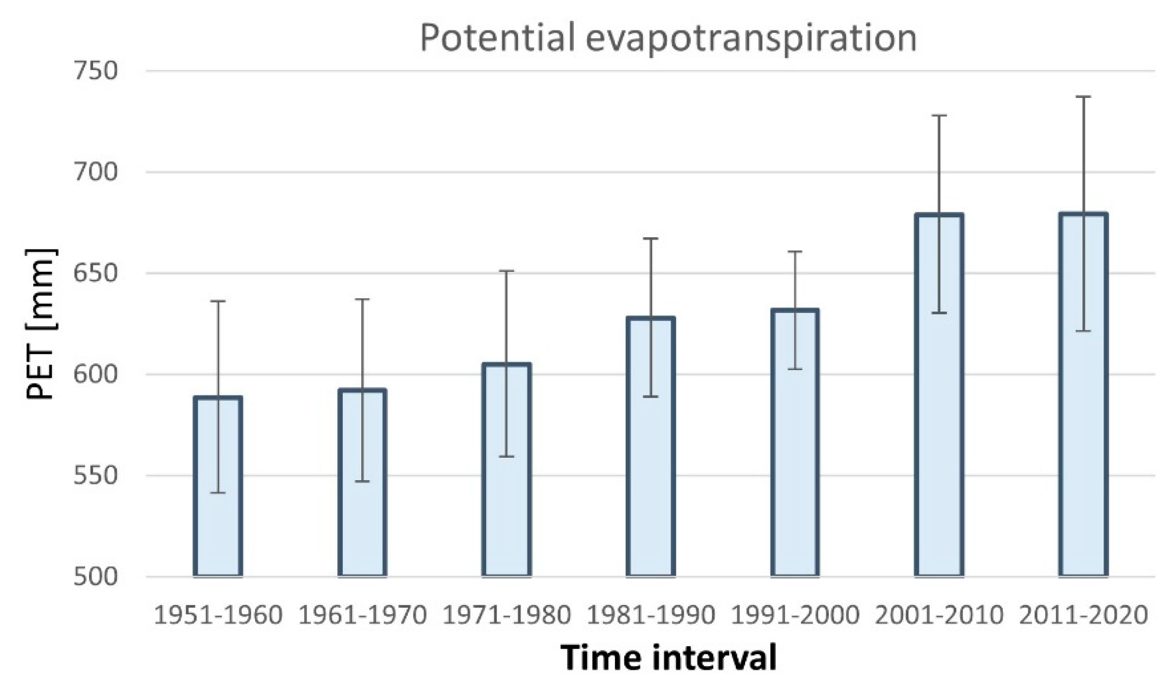
The observed increase in air temperature contributed to the increase in potential evapotranspiration. In particular, in the 2011–2020 period, a large increase in potential evapotranspiration was found and the variability of this indicator increased (
Figure 1).
In recent decades, changes in the climate have been observed in Poland, resulting from warming, changes in precipitation, and a number of extreme weather events [
7,
8,
9]. Climate change scenarios developed by the IPCC [
10] indicate a 10-fold increase in the occurrence of droughts in Poland in the coming decades [
11]. According to NOAA, 2017 was the second warmest year of meteorological recording and analysis (since 1880) in the world [
12]. By analyzing the climate scenarios for the years 2021–2050, it has been shown that the growing season in Poland, defined by the number of days with the daily air temperature 5 °C higher in the years 2021–2050, will be longer than in the years 1971–2000 by 16 days. The predicted higher temperature in the growing season of plants will significantly accelerate their development [
2]. Therefore, it is necessary to look for solutions to minimize the negative impact of climate change [
13], e.g., the occurrence of weather extremes and droughts [
6,
14,
15,
16,
17] in the Bystra catchment areas, in the coming decades. In order to assess the effectiveness of the proposed solutions, it is necessary to develop boundary conditions, indicating a baseline representing the behavior of the Bystra catchment hydrosystem in the ‘business as usual scenario’ (i.e., taking into account changes in the hydrological cycle caused only by climate change with unchanged conditions of human activity). The above-mentioned boundary conditions for the 2050 horizon must be based on simulation modeling, calibrated on archival data. One of the many mathematical models suitable for the analysis of the water balance of the catchment area and the analysis of the impact of predicted climate changes in the future decades is the SWAT model.
This study uses large scale application SWAT for Vistula and Odra large catchment-based analysis to determine increases of both low and high river flows [
18]. It was also shown that soil moisture and soil physical properties add valuable information for the prediction of climate change impact on yield variability [
18].
The purpose of this article is to prepare an appropriate SWAT model and to study spatial assessment of hydrological indices obtained in three varied climate projections for two representative concentration pathways (RCPs) in order to analyze differences in the results of regional climate models based on the same global climate model [
19]. These models are characterized by different parameterization of physical processes while running on the same spatial domain, covering the European continent, and benefiting from the boundary and initial conditions of the same global model (EC-EARTH). Such assessment attitudes matter for future research on the effectiveness of agricultural land use change adaptation practices in terms of reducing water erosion and increasing water retention in the landscape, including small retention, introduced in various variants related to land consolidation.
The developed model, after calibration and validation, was used for research related to the prepared projections for the RCP 4.5 and RCP 8.5 scenarios.
The study area was selected due to the large relief and the predominance of soils made of loess. The agricultural nature of the catchment area and loess soils with good retention properties [
20] will be used in subsequent publications to assess adaptation scenarios. The Bystra catchment area has been the target of many studies and statutory re-search by IUNG. The results of these studies have been used in this present study.
Due to the observed temperature increase, which also contributes to the increase in potential evapotranspiration in recent years, the years 2010–2017 were adopted for the SWAT model.
The aim of the article is to analyze the hydrology of the Bystra River basin in the 2021–2050 climate projections for the RCP 4.5 and RCP 8.5 climate change scenarios, as well as to provide an assessment against the background of the current state of knowledge related to research covering the European continent and small regional catchments.
2. Study Area
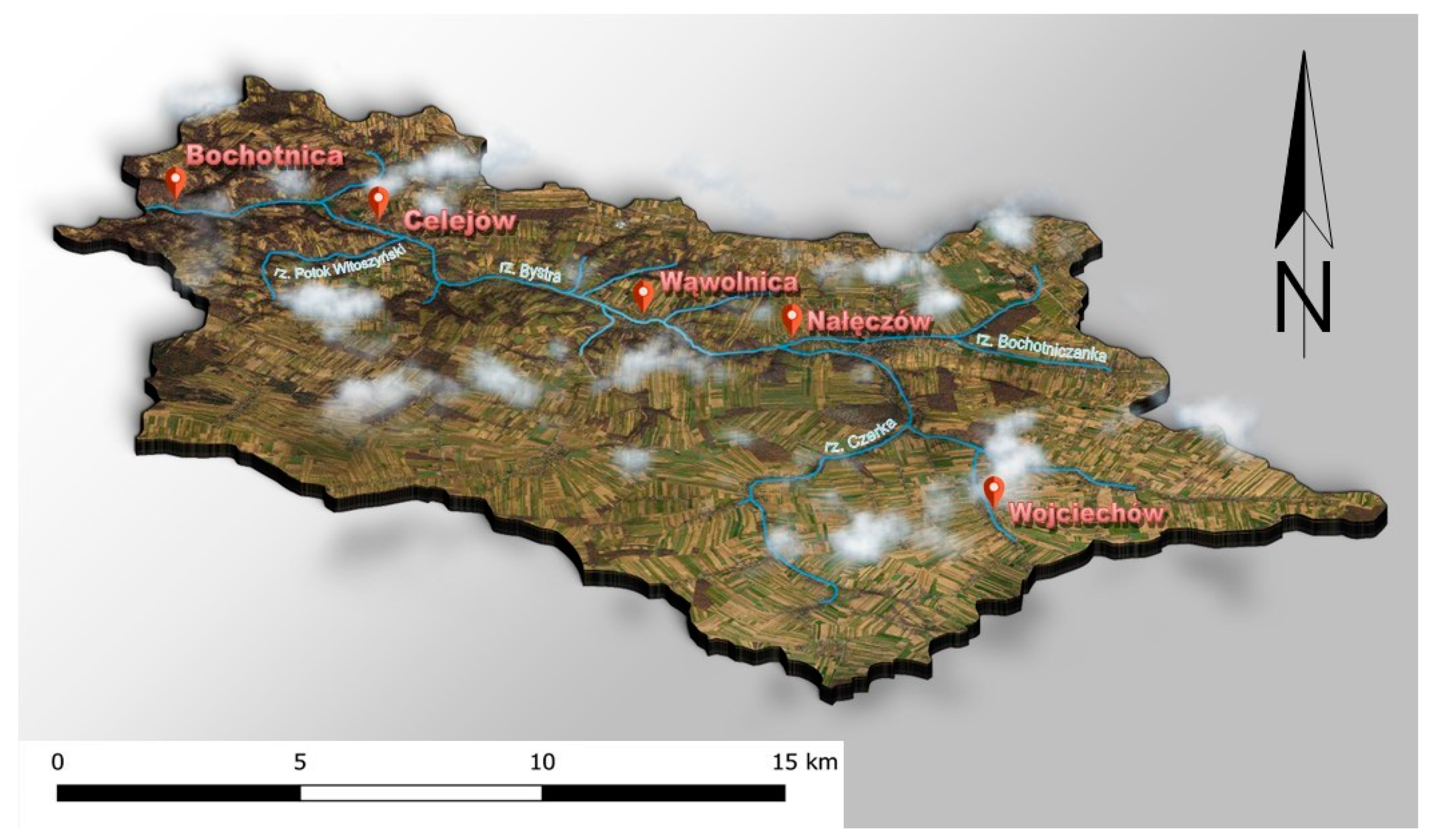
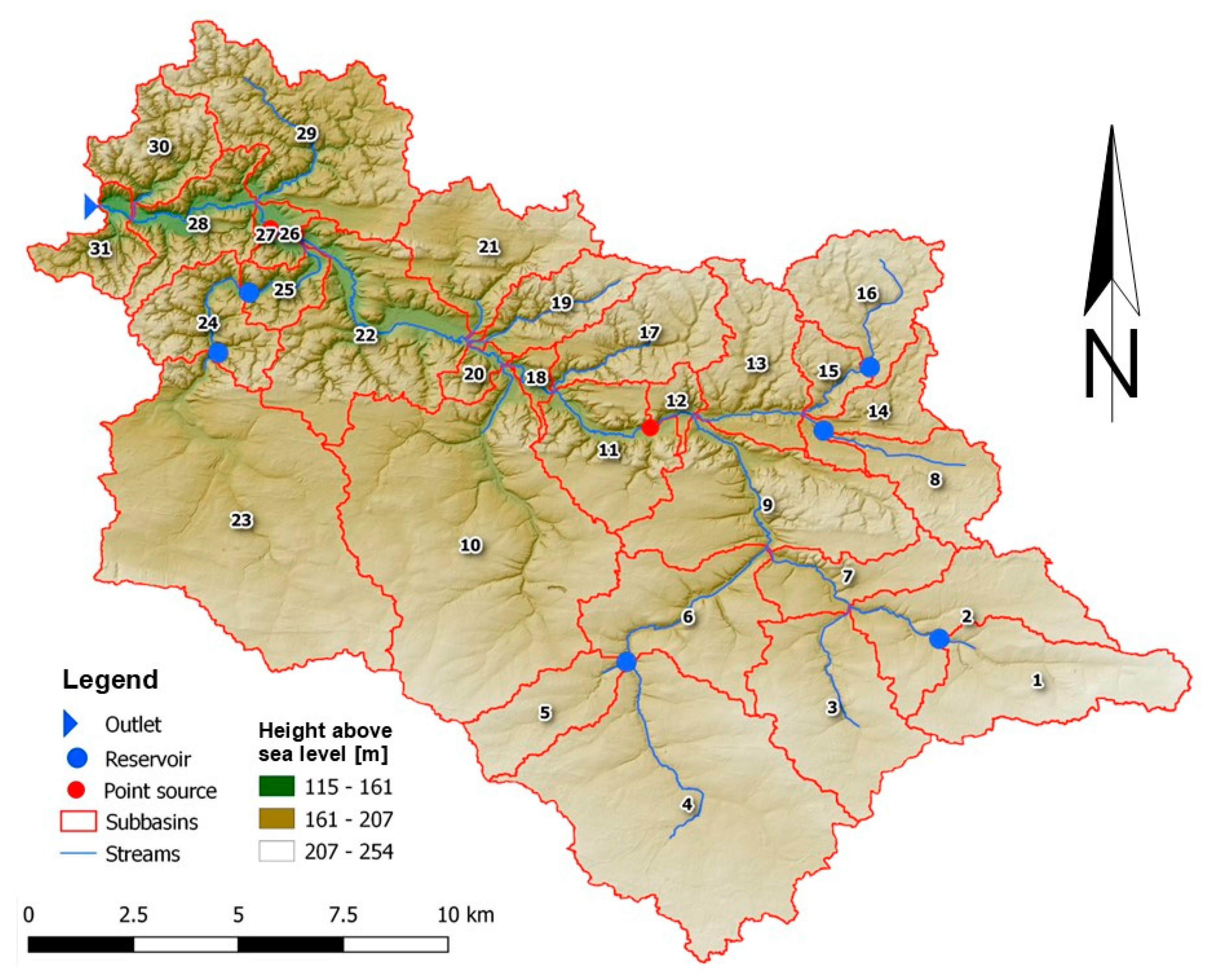
The Bystra River, which is the right tributary of the Vistula River, 33 km long and 306.9 km
2 in area, is located in the Lubelskie Voivodeship (
Figure 2). The Bystra River basin is a second order hydrographic unit (Code PLRW2000923899) [
21]. According to the generated SWAT model, the lowest point of the catchment area is 123 m above sea level, while the highest point is 246 m above sea level. The catchment area is 296.6 km
2.
The Bystra River basin part of the Lublin Upland [
22,
23,
24] The relief of the Bystra River valley and its tributaries is very large and consists of many valley forms with a constant or episodic inflow. There are few valleys with a constant tributary. The largest of them, the Bystra valley, is 35 km long. In the section where the Bystra River valley flows into the Vistula, it cuts up to 35 m in marl and rocks [
21,
25,
26].
Virtually the entire catchment area is built of a deep loess (up to 20 m). In the deeper layers there are Quaternary Pleistocene deposits, glacial sands and gravels, and slightly deeper tilts. Paleocene Paleogene deposits lie under the clay (i.e., geoses). On the other hand, under the geezes there are upper Cretaceous deposits (i.e., rocks with limestone inserts) [
27].
The upland nature of the catchment area with a predominance of loess soils and the high slopes of the slopes at the mouth of the Bystra River pose a significant threat to the catchment area in terms of medium and very strong water and surface erosion [
28].
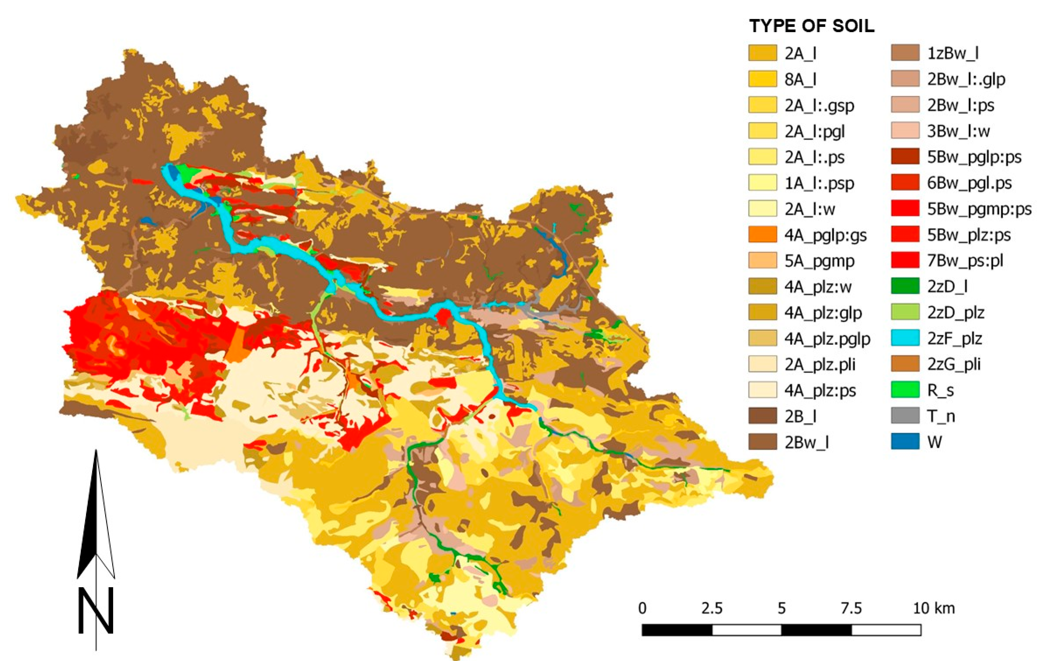
According to the raster soil map prepared for the SWAT model (
Figure 3), the study area consists mainly of podzolic and pseudo-polygonal soils (49%) as well as leached brown soils and acid soils (47%) (
Table 1).
Overall, 32 grain size groups were separated. Podzolic soils extend mainly in the south-eastern area of the catchment area, while brown soils dominate in the north-west area. Loess (73%) [
29,
30,
31] and ordinary dust (18%) dominate in the soil cover of the Bystra River catchment area.
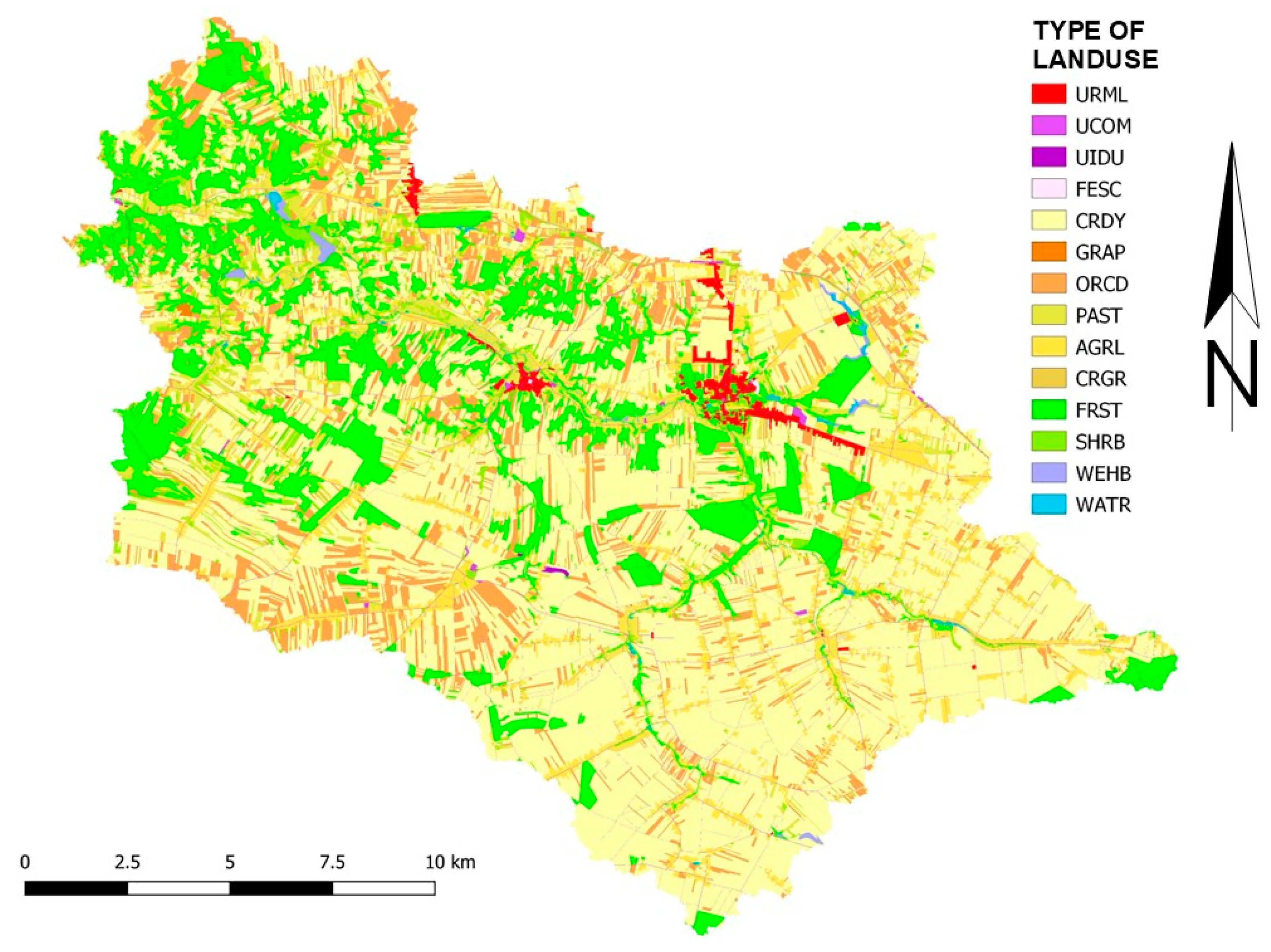
According to the map of the cover and land use of the Bystra River catchment area, arable lands (78%) and forests (16%) dominate (
Figure 4).
The largest part of agricultural land is arable land beyond the range of irrigation facilities (52%), a large area is also orchards and plantations (11%), complex systems of cultivating plots (9%) and meadows and pastures (6%) (
Table 2).
3. Methods
3.1. SWAT and SWAT-CUP
In order to examine the water balance of the Bystra River catchment area, the soil and water assessment tool (SWAT) model was used [
32]. The SWAT model can be used with a variety of computer programs. For the purpose of this article, the QSWAT3 v1.1 model with interface in Quantum GIS 3.10.13 Coruna [
33] was used. SWAT Editor 23 October 2012 software [
34] was used for model calculations. The SWAT model is a deterministic model developed for the US Department of Agriculture [
35] that is based on mapping physical, chemical, and biological processes using mathematical formulas, developed to predict the effects of management practices on water and agricultural chemical yields on a basin scale [
36,
37].
The water balance is the basis and the driving force behind all of the processes that take place in the catchment area, regardless of the type of analysis performed with the use of the SWAT model [
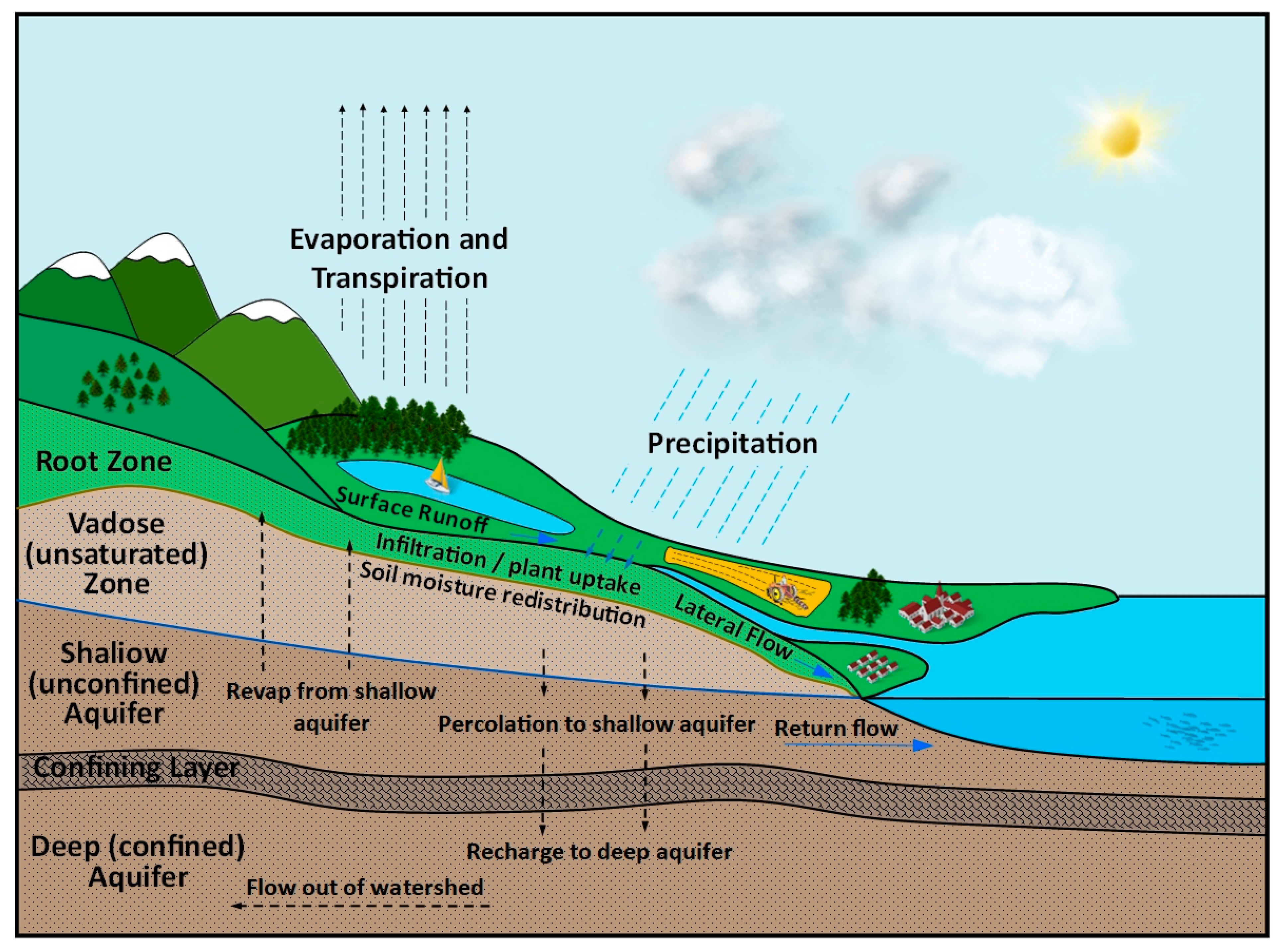
38]. The modeling of the watershed is carried out in two phases: a land phase and routing phase. The land phase of the hydrological cycle [
39] controls the amount of water, sediment, nutrients and pesticides entering the main canal in each catchment area. The land phase of the hydrological cycle controls the amount of water, sediment, nutrients, and pesticides introduced into the main canal in each catchment area, covering long periods of time with a time resolution of one year, month, or day (
Figure 5).
Routing phase of the hydrologic cycle which can be defined as the movement of water, sediments, etc. through the channel network of the watershed to the outlet. The hydrologic cycle can be defined as the movement of water, sediments, etc. through the channel network of the watershed to the outlet [
40]. The simulated processes include the cycles of nitrogen, phosphorus, carbon, pesticides, bacteria, and metals. Above the processes are related in the SWAT model with the plant growth cycle and catchment management practices (e.g., plowing, fertilization, harvesting plants, irrigation of fields, collection and transfer of water, drainage of water and sewage, use of home sewage treatment plants, and buffer zones along watercourses) [
32,
41].
The land phase estimates the runoff for each of these HRUs using the water balance equation:
where
SWt is the final soil water content (mm);
SW0 is the initial soil water content (mm);
t is time in days;
Pd is precipitation (mm);
SURQ is surface runoff (mm);
E is the evapotranspiration (mm);
wseep is amount of water entering the vadose zone from the soil profile (mm); and
GWQ is groundwater flow (mm) [
40].
The SWAT model used the Penman–Monteith method to assess potential evapotranspiration.
To better adjust (calibrate) the SWAT model to the actual conditions in the Bystra river catchment area, SWAT Calibration and Uncertainty Programs 5.2.1 [
42] were used. The SWAT-CUP program is an instrument used to calibrate, analyze the uncertainty and sensitivity of the SWAT model [
42,
43]. The SUFI-2 algorithm was used since it works well for small catchments [
44,
45,
46].
3.2. Data Used in the SWAT Model
To simulate the water balance in the SWAT model, spatial data were obtained from many sources, including:
- -
A digital elevation model covering the catchment area with a resolution of 5 m, obtained from the Central Geodetic and Cartographic Documentation Center [
47];
- -
Data on the hydrography of the area (e.g., rivers, lakes, partial catchments), which were obtained from the Polish Hydrological Division Computer Map with descriptions [
48];
- -
Data on sewage treatment plants [
49];
- -
Digital soil and agricultural maps in digital form (scale 1:25,000 and 1:100,000) [
50]; which were obtained from the Institute of Soil Science and Plant Cultivation in Pulawy [
51];
- -
Geological data describing lithology obtained from the Polish Geological Institute in the form of a Detailed Geological Map of Poland [
27];
- -
Types of land cover and land use, digital data obtained from Corine Land Cover databases [
52];
- -
A high-resolution orthophoto map published on the Geoportal in the form of WMS [
53];
- -
Open Street Map data [
54];
- -
Meteorological data obtained from IUNG in Pulawy and the Institute of Meteorology and Water Management [
55].
3.3. Adaptation of the SWAT Model for the Study Area
In the first stage, the input data for the precipitation-outflow system was prepared for SWAT modeling. Based on the digital elevation model and the location of the lakes in the studied area and water discharges from the wastewater treatment plant, a division of the Bystra River basin into partial catchments was generated in the SWAT editor. The editor generated 31 partial catchments (
Figure 6). According to MPHP, the catchment area of the Bystra River consists of 21 sub-basins. The increased number of partial catchments is related to selecting points representing reservoirs and points source, for which additional data will be entered at a later stage. The above points must be located as close as possible to the line representing the river network. There are also many water reservoirs, ponds, and ponds in the sub-catchments that are not related to the watercourse line. These are the objects for which additional data will also be entered, representing all water reservoirs in the sub-catchment.
In the next stage of creating the SWAT model, hydrologic response unit (HRU) areas had to be generated, HRUs are homogeneous hydrological areas created on the basis of overlapping land cover maps, soil maps and slope maps [
40].
For the needs of the SWAT model, a soil map of the Bystra catchment was developed based on digital soil and agricultural maps (scale 1:25,000 and 1:100,000) and geological data describing lithology. Data describing the parameters of the soils in the Bystra river catchment area were obtained as part of the statutory projects of IUNG-PIB [
21].
During the preparation of soil data, it was also taken into account that the available water capacity and wilting point values were appropriate for the soils of the Bystra catchment area. These values were obtained from the study “Assessment of Water Retention in Soil and the Risk of Drought Based on the Water Balance for the Area of the Lower Silesia Voivodship”, developed in 2013 by the employees of the Department of Soil Science, Erosion, and Land Protection IUNG-PIB in Pulawy [
20].
Due to the low detail of the Corine Land Cover map, additional vectorization of the cover and land use of the Bystra River catchment area was performed in order to increase the resolution of land use using an orthophoto map and Open Street Map data.
For the Bystra River catchment area, a division was also made due to the decline in the area in the following ranges: 0–6%, 6–10%, 10–18%, 18–27%, >27%. Slope ranges originate from the PWER and AWER indicators [
56] for soil erosion risk, remaining as standard in terrain relief visualization in Poland. The Bystra River catchment area is similar to that of the Grodarz catchment area to the south, which has the same slope distribution. [
57,
58]. The Bystra River basin is similar in relief to the Grodarz River basin. In the studied catchment area, flat and slightly undulating areas with slopes up to 6% (72% of the catchment area) prevail. Steep slopes, from 6% to 10%, account for 11% of the catchment area. A small area of the catchment area is represented by land with falls from 10% to 27% (11%). A total of 6% of the catchment area are falls over 27%.
After preparing the rasters for soil, land cover, and slopes, the catchment area was divided into HRU areas in the SWAT program.
During the creation of HRU in the SWAT program, the percentage of arable land outside the range of CRDY irrigation devices was separated from winter crops WWHT (43%), spring BARL crops (31%), canola CANP (14%) and other CRDY (12%), based on the publication Agriculture in the Lubelskie Voivodeship in 2019 [
59]. From fruit orchards, ORCD was separated on the basis of the above-mentioned APPL apple orchards publication. Forests, on the other hand, were divided into coniferous FRSE forests (49%), deciduous FRSD forests (13%) and mixed FRST forests (38%) according to information obtained from the Regional Directorate of State Forests in Lublin [
60].
A total of 484 HRU areas were generated. The HRU areas will be used at a later stage to build the SWAT model.
3.4. Meteorological Data
In the next stage of creating the SWAT model, the following meteorological data had to be loaded: sums of daily precipitation [mm]; daily minimum and maximum air temperature [°C]; average daily wind speed [m/s]; daily mean relative humidity; daily sums of total solar radiation [MJ/m
2]. Meteorological data were obtained from Pulawy weather station (
Table 3). The data were prepared in SWAT Weather Database 0.18.03 [
61].
In the last stage of the SWAT model construction, some parameters related to point sewage discharges concerning water reservoirs outside the river network, concerning reservoirs, and parameters scheduled management operations for non-irrigated arable land were supplemented and corrected.
The parameters of rivers in the sub catchments were also improved on the basis of data obtained as part of the statutory projects of IUNG-PIB, as the automatically generated parameters of rivers regarding the length, depth, and width of the rivers were overestimated.
The current value of CO2 concentration was also inserted in the prepared SWAT model.
After entering all of the necessary data into the SWAT model, a simulation of the water cycle in the Bystra River catchment was performed for 2010–2017 with a five-year model start-up period, in a monthly step.
3.5. SWAT CUP Calibration and Validation Results
After the SWAT simulation, the obtained model had to be calibrated in the SWAT-CUP program [
62,
63,
64] to obtain a more accurate representation of the model with reality. For this purpose, data on average monthly flow velocities [m
3/s] in the vicinity of the estuary of the Bystra River basin to the Vistula for the years 2010–2014 were used, obtained under the statutory projects of IUNG-PIB. After receiving a satisfactory calibration, the model was validated using the data on the monthly average flow velocities [m
3/s] near the mouth of the Bystra River basin to the Vistula for 2015–2017, obtained under the statutory projects of IUNG-PIB. Calibration and validation were performed in a monthly step.
As a result of the calibration in the SWAT-CUP software, the best-fit parameter ranges were obtained that meet the accuracy requirements of calibration and validation [
43,
65,
66].
The figure shows only the months which the water discharge was recorded and compared to the values simulated in 95 Percent Prediction Uncertainty (
Figure 7). For the performed calibration and validation, there are data gaps in the measurements covering the periods from December 2010 to March 2013, September 2013 to January 2014, March 2015, July and August 2016, and from October 2016 to February 2017 and September 2017.
In addition to the above-mentioned best fit parameters, there are other parameter sets that can also give a good calibration result [
63].
The Nash-Sutclif model efficiency coefficient (NSE) for calibration is in the range of 0.5 < NSE ≤ 0.65 and is a satisfactory result. The coefficient of determination R
2 is also within the acceptable range of 0.5 < NSE ≤ 0.65 [
65]. The Nash-Sutclif model efficiency coefficient for the validation is in the range of 0.65 < NSE ≤ 0.75, which is good result. The coefficient of determination R
2 is in the range of 0.5 < NSE ≤ 0.65. This is also a satisfactory result [
65].
For the performed calibration and validation, there are data gaps in the measurements covering the periods from December 2010 to March 2013, September 2013 to January 2014, March 2015, July and August 2016, from October 2016 to February 2017 and September 2017.
An important aspect is the appropriate consideration of the flow measurement period for validation and calibration. When preparing the data, the measurement data should be selected so that they cover a homogeneous period of time in terms of constant weather conditions. When preparing the data for the SWAT model, a distinction is made between the so-called dry and wet years. If there are measurement series covering dry and wet years, then calibration and validation may be difficult [
67].
During the analysis of the results, the obtained values of potential evapotranspiration were also compared with the results of statutory IUNG-PIB research conducted as part of the Agricultural Drought Monitoring System project [
68]. The SWAT model is a good representation of potential evapotranspiration in the studied area. In addition, the results of soil water content were compared with the available water capacity and wilting point values obtained from the study “Assessment of Water Retention in Soil and Drought Risk Based on the Water Balance for the Lower Silesian Voivodeship”, developed in 2013 by employees of the Department of Soil Science, Erosion and Land Protection. IUNG-PIB in Pulawy [
20].
3.6. Climate Change Scenarios
The daily gridded climate data for the period (2020–2050) with a spatial resolution of 0.11° were obtained from the EURO-CORDEX database that are openly available through the ESGF (Earth System Grid Federation,
https://esgf-data.dkrz.de/search/cordex-dkrz, accessed on 10 February 2022) for Europe [
69,
70]. Climate projections (of daily minimum and maximum air temperature, precipitation, surface downwelling shortwave radiation, wind speed, relative humidity) that were used in SWAT model were extracted from grid cells that corresponds to the weather station’s location. The projections are based on three regional climate models (RCMs) and two Representative Concentration Pathways (RCP). The RCMs (Regional Climate Models) were: RACMO22E, HIRHAM5 and RCA4 driven by one GCM (General Circulation Model): EC-EARTH. The RCPs correspond to a radiative forcing value in the year 2100 relative to pre-industrial values of +4.5 W m
−2 (RCP4.5), while RCP8.5 to + 8.5 W m
−2 (RCP8.5) [
71,
72] (
Table 4).
In total we used six climate projections (three RCMs × two RCPs). The air temperature and precipitation data were additionally bias adjusted by the SMHI (Swedish Meteorological and Hydrological Institute) using DBS (distribution-based scaling) method [
73] and regional reanalysis MESAN (mesoscale analysis) dataset from period 1989–2010 [
74]. Since the downloaded data were performed on the rotated polar grid, we applied bilinear interpolation to remap this dataset to regular geographic latitude/longitude grid by using CDO (climate data operators) software [
75].
For the control period of the results of climate projections (RCP 4.5, RCP 8.5), validation was performed with existing observation data of temperature and precipitation (
Table 5). The range of differences between the temperatures varies from 0.3 to 0.7 degrees Celsius in the plus. On the other hand, the differences for the climate projections in the control years 2010–2017 are smaller than 11% to 22% percent compared to the observational data.
The prepared model, after calibration and validation, was used for research related to the RCP 4.5 and RCP 8.5 climate change scenarios (changes in carbon dioxide concentration in the future decades) [
70,
76,
77] which scenarios have been accepted by the International Panel on Climate Change [
78].
For each of the projections, there is a certain confidence interval of the flow result obtained in the SWAT-CUP program. In order to compare the climate change scenarios for individual climate projections (RCP 4.5.1, RCP 8.5.1, RCP 4.5.2, RCP 8.5.2, RCP 4.5.3 and RCP 8.5.3), one iteration was carried out in SWAT-CUP for the best calibration parameters for 2020–2050 for prepared scenarios (
Table 4). Additionally, for the RCP 4.5 and RCP 8.5 scenarios, changes in CO
2 concentrations in individual decades were adopted: 2021–2030, 2031–2040 and 2041–2050, developed by the Potsdam Institute for Climate Impact Research [
79,
80].
4. Average Annual Prospects of Climate Scenarios RCP 4.5 and RCP 8.5 for the Period 2020–2050
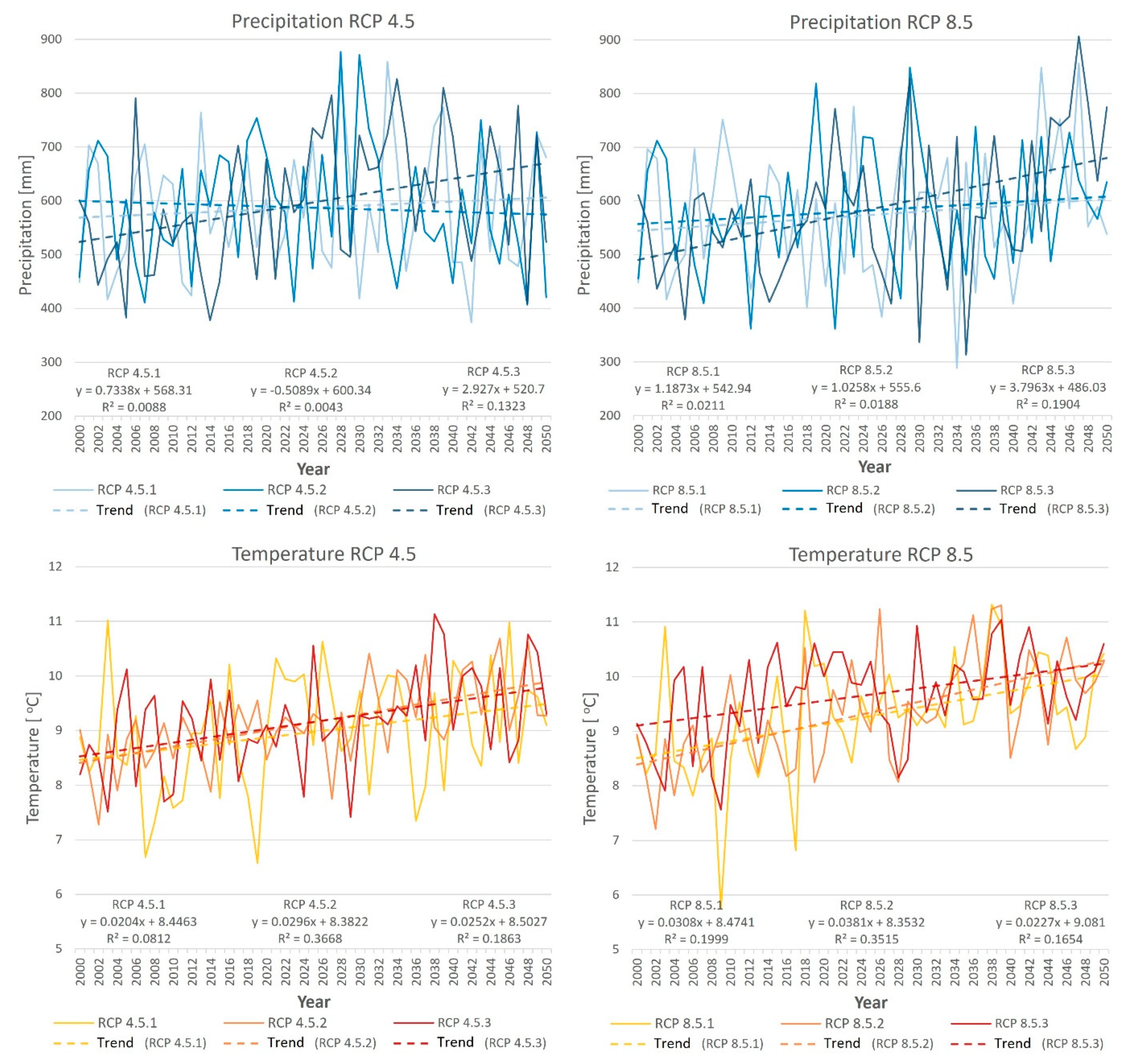
The average annual sum of precipitation and the average annual temperature in the years 2000–2050 are different for different projections in the RCP 4.5 and RCP 8.5 climate scenarios (
Figure 8). For the projection RCP 4.5.1, RCP 8.5.1, and RCP 8.5.2 the trend of average annual precipitation will be slightly increasing in the following years. On the other hand, for the RCP 4.5.2 projection, the trend of average annual precipitation totals will be slightly decreasing. For the RCP 4.5.3 and RCP 8.5.3 projection, the trend of average annual precipitation totals will be increasing.
For the RCP 4.5 and RCP 8.5 scenarios, all three forecasts will see an increase in the annual mean temperature trend in the coming decades.
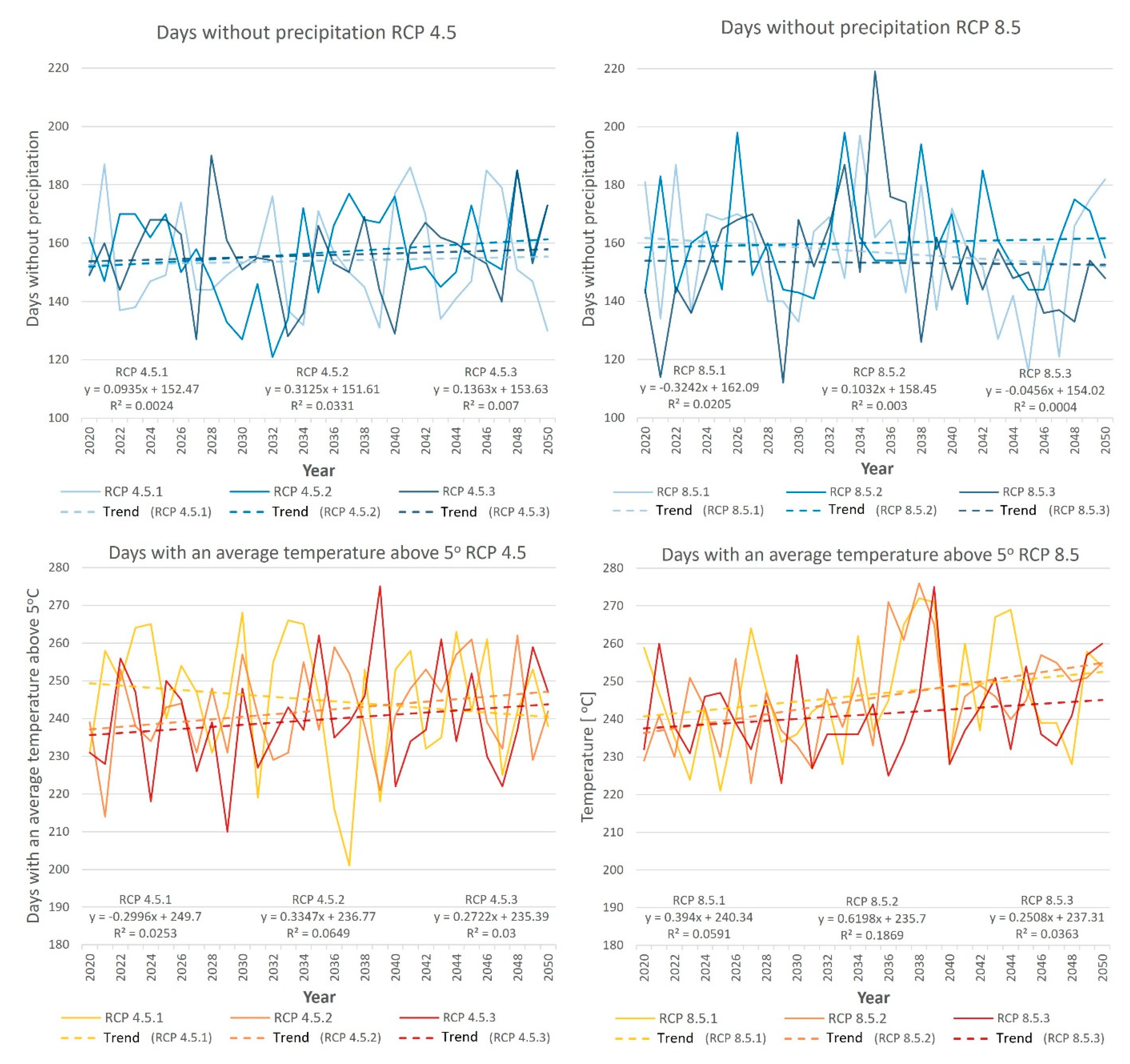
The trend of the average annual number of days without precipitation for the RCP 4.5 scenarios for all projections and for the RCP 8.5.2 projection are positive. However, in the case of RCP 8.5.1 and RCP 8.5.3 there is no trend line (
Figure 9).
The trend of the average annual number of days with an average temperature above 5 °C in the years 2020–2050 for most climate projections is positive, apart from the RCP 4.5.1 projection.
The average monthly sums of precipitation for the Bystra River basin in the simulation years 2010–2017 and change in the individual climate change projections in the years 2021–2030, 2031–2040, and 2041–2050 are shown in
Table 6. These changes are especially visible in March, August, and November, where for most of the projections there is an increase in the average monthly precipitation.
On the other hand, the decrease in average monthly sums of atmospheric precipitation will occur in most of the projections in January, May, July, and October.
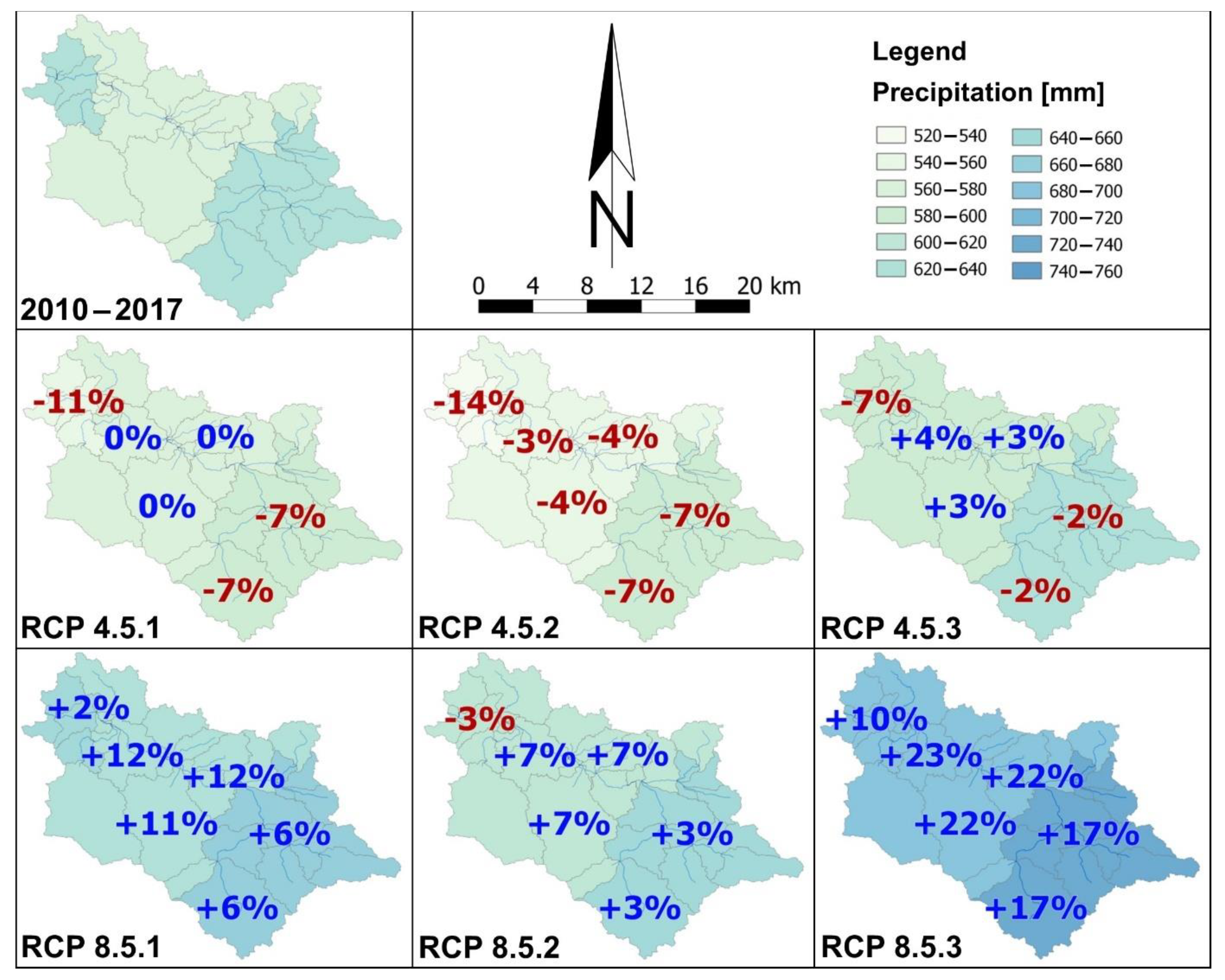
For most of the projections, the average annual precipitation will be lower in the next decades as compared to 2010–2017. Larger annual mean sums will appear in the forecasts RCP5.1 (2031–2040), RCP 4.5.2 (2021–2030), RCP 4.5.3 (2021–2030, 2031–2040, 2041–2050), RCP 8.5.2 (2021–2030, 2041–2050), RCP 8.5.1, and RCP 8.5.3 (2041–2050).
Annual averages for RCP 2041–2050 for RCP 4.5 are lower by 3%, while for RCP 8.5 they are higher by 11% compared to the lower period.
By analyzing the spatial distribution of changes in the average annual precipitation total in 31 sub-catchments for the simulation period in 2010–2017 compared to the period 2041–2050 (
Figure 10) in the RCP 4.5.1 and RCP 4.5.3 climate projections, the precipitation total will decrease by several percent in north-west and south-east region. In the RCP 4.5.2 projection, a reduced amount of precipitation will occur in the entire catchment area, while in the RCP 8.5.2 projection it will occur only in the northwestern part. In projections 8.5.1 and 8.5.3, an increased amount of precipitation, up to 23%, will be present in the entire area in the period 2041–2050. Most of the RCP 8.5.2 area will also have an increased amount of precipitation.
The average monthly temperature distributions for the Bystra River basin in the 2010–2017 simulation years also change compared to the individual climate change projections in 2021–2050 (
Table 7). These changes are especially visible in November and December, where for most of the projections the average monthly temperature is lower than in the 2010–2017 simulation period. On the other hand, in January, April, May, September, and October, the average monthly temperatures are higher for most of the projections. For the RCP 8.5.2 (2031–2040, 2041–2050) and RCP 8.5.3 (2041–2050) projections, the average monthly temperatures for most months are higher than in the 2010–2017 simulation years.
The temperature in the 2041–2050 decade for RCP 4.5 will be higher by an average of 0.4 °C, while for RCP 8.5 it will be higher by an average of 0.8 °C compared to the simulation period.
5. Results
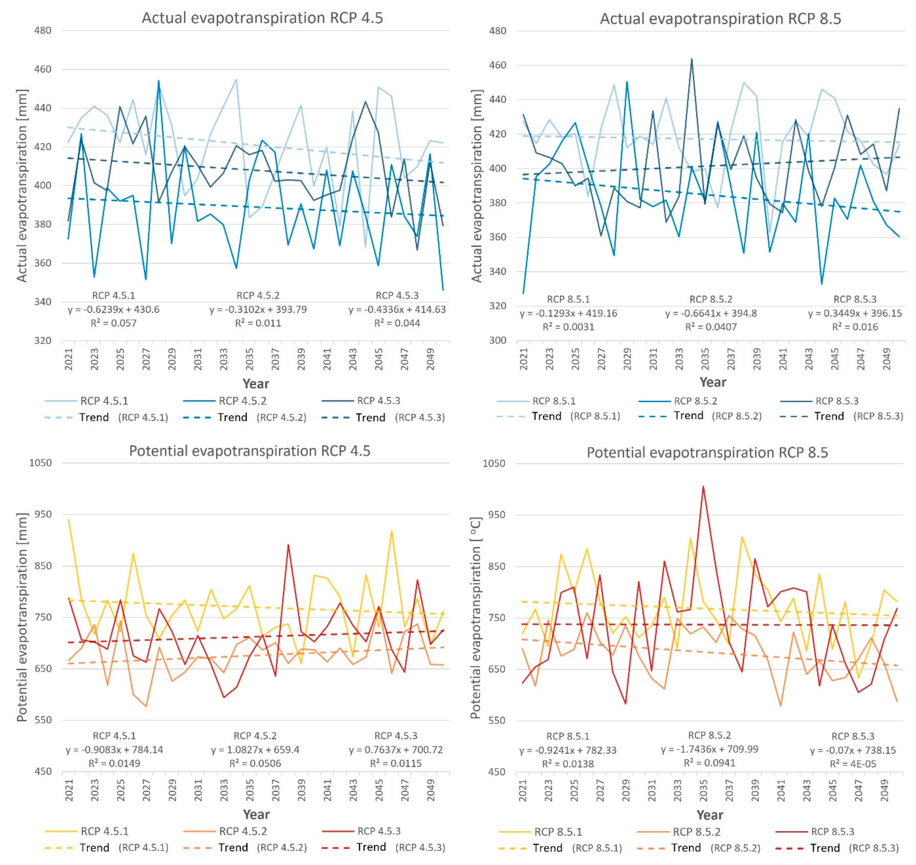
The trend of the average annual sum of actual evapotranspiration in the years 2021–2050 in most of the projections (except for RCP 8.5.3) decreases slightly in the coming decades (
Figure 11).
The trend of the average annual sum of potential evapotranspiration in RCP 4.5.1, RCP 8.5.1 and RCP 8.5.2 projections will decrease in the coming decades. However, for the RCP 4.5.2 and RCP 4.5.3 projections, the trend is growing. The trend line for the RCP 8.5.3 projection does not change significantly.
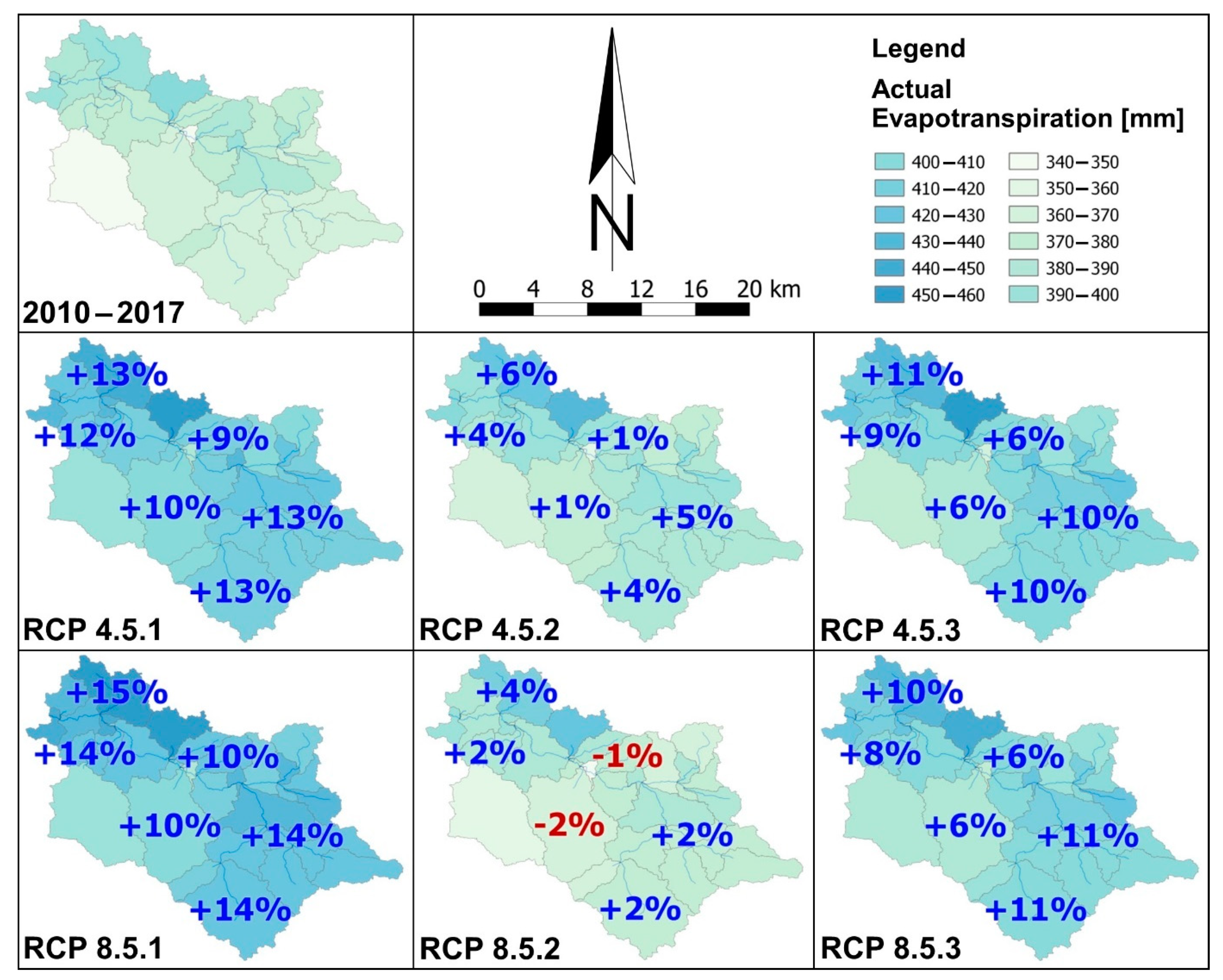
The average monthly sum of actual evapotranspiration increases for all projections for most months compared to the simulation period 2010–2017. In June, for most projections, the average monthly sum of evapotranspiration will be lower than the average for 2010–2017 (
Table 8).
The average annual potential evapotranspiration in the 2041–2050 decade for RCP 4.5 will be higher by an average of 8%, while for RCP 8.5 it will be higher by an average of 8% compared to the simulation period.
For potential evapotranspiration, the average monthly sum increases for most of the projections in all months compared to the 2010–2017 simulation period (
Table 9).
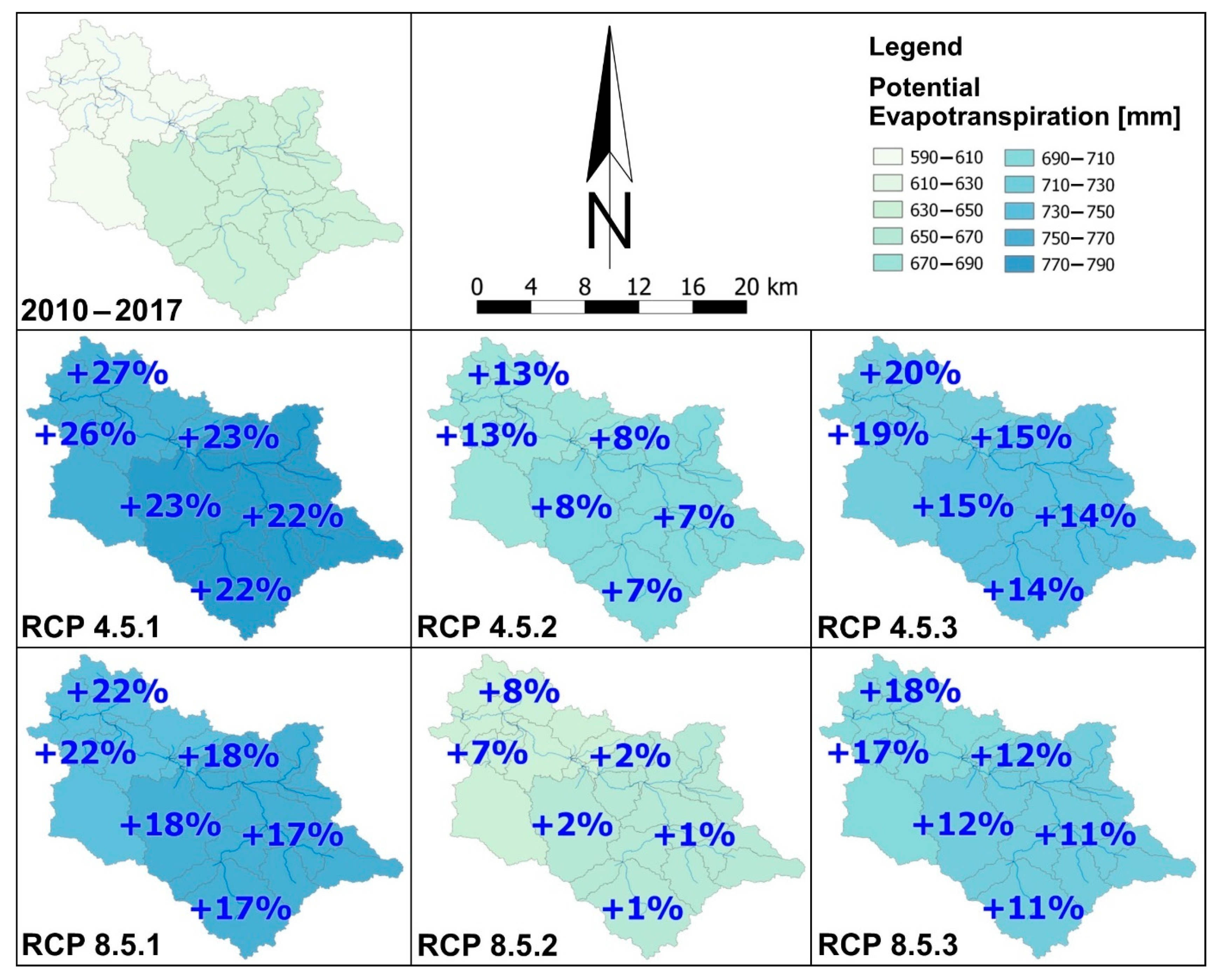
The average annual potential evapotranspiration in the 2041–2050 decade for RCP 4.5 will be higher by an average of 12%, while for RCP 8.5 it will be higher by an average of 17% compared to the simulation period.
By analyzing the spatial distribution of changes in the average annual sum of actual evapotranspiration in 31 sub-catchments for the simulation period in 2010–2017 compared to the period 2041–2050 (
Figure 12) for most projections, actual evapotranspiration will increase. Only for the projection of RCP 8.5.2 in the central part of the Bystra catchment area, the sum of actual evapotranspiration will be lower than in the simulation period.
Spatial distribution of changes in the average annual sum of potential evapotranspiration in 31 sub-catchments for the simulation period in 2010–2017 compared to the period 2041–2050 (
Figure 13) for all projections, the potential evapotranspiration will increase. The largest increase will be recorded in the RCP 4.5.1 and RCP 8.5.1 projections, reaching even 27% in the north-western part of the catchment area.
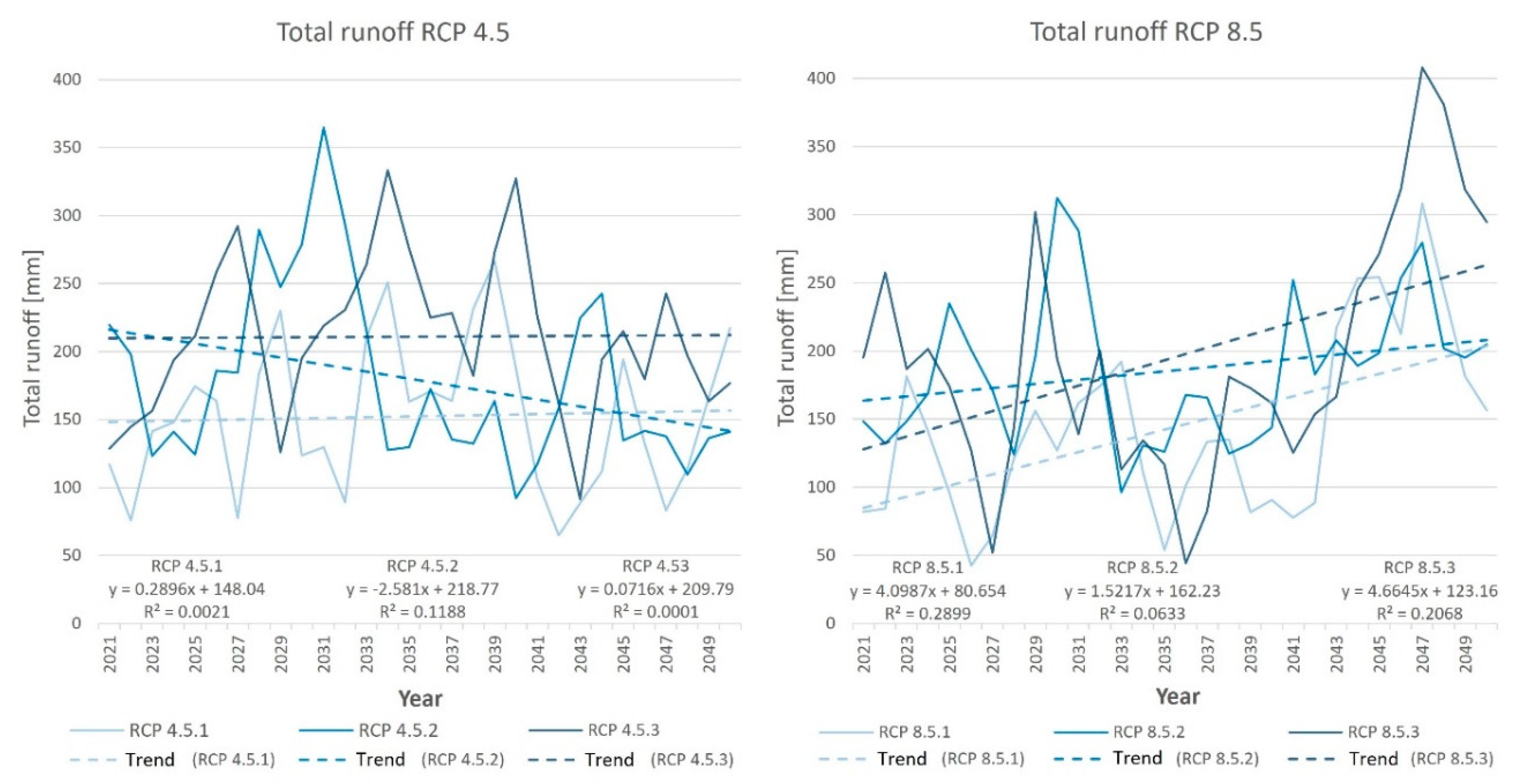
The trend of the average annual total runoff consisting of surface runoff, lateral flow and baseline flow in the RCP 8.5.1, RCP 8.5.2, and RCP 8.5.3 projections will increase over the years 2021–2050 (
Figure 14). For the RCP 4.5.2 projection, the trend will be downward. However, for the RCP 4.5.1 and RCP 4.5.2 projections, the trend will not change significantly.
The average monthly total runoff for the Bystra River basin will be lower in most climate change projections in the years 2021–2030, 2031–2040, and 2041–2050 (
Table 10). The exceptions will be the RCP 4.5.3 (2031–2040) and RCP 8.5.2, RCP 8.5.3 (2041–2050) projections, where the average total monthly runoff will be higher compared to the 2010–2017 simulation years.
The average annual total runoff in the decade 2041–2050 for RCP 4.5 will be lower by an average of 23%, while for RCP 8.5 it will be higher by an average of 13% compared to the simulation period.
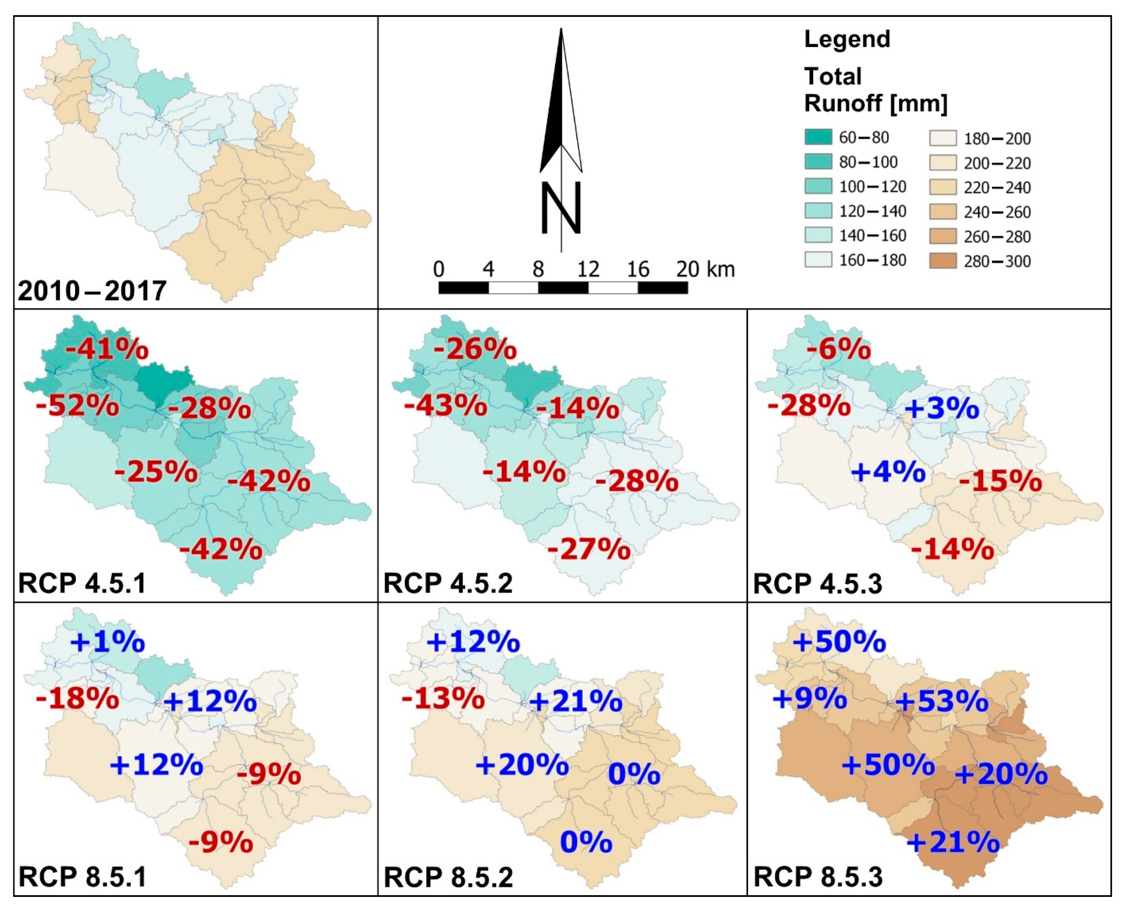
When analyzing the spatial distribution of changes in the average annual total runoff in 31 sub-catchments for the simulation period in 2010–2017 compared to the period 2041–2050 for the RCP 4.5.1 and RCP 4.5.2 projections, the average annual total runoff amount will be lower in the entire catchment area, even reaching up to 52% (
Figure 15). For RCP 4.5.3, total runoff will be lower in the northwest and southeast. It will be higher in the central part. RCP 8.5.1 and RCP 8.5.2 will have runoff volumes varying depending on the catchment area. On the other hand, the projection of RCP 8.5.3 for the whole area will have the average annual total runoff higher than in the simulation period.
6. Discussion
The analysis of the climate for the years 1970–2004 shows a statistically significant increase in the sum of evapotranspiration in the growing season. In the years 2021–2030, 2031–2040, and 2041–2050, an increase in potential evapotranspiration during the growing season is also shown (
Table 8) [
81]. Moreover, the amount of precipitation increases in winter and early spring and decreases in spring and summer. Changes in the temporal structure of precipitation may cause an increase in soil moisture in spring, which may affect areas at risk of water erosion where surface runoff should be regulated (especially on dirt roads). This contributes to lowering the climatic water balance (i.e., increasing the precipitation deficit in relation to potential evaporation) [
2,
82]. Reducing the amount of precipitation, evapotranspiration, and extending the growing season caused by the temperature increase in the summer period may increase water shortages for plants [
1,
2].
The climate projection for Poland [
82] for the years 2021–2030, 2031–2040, and 2041–2050 shows increased values of precipitation in summer (except for 2041–2050) and in autumn for the RCP 4.5 scenario compared to the period 2011–2020. However, in spring, precipitation will be lower for all decades (
Table 11). Similar results were obtained for the average precipitation data in the RCP 4.5 scenario for the years 2021–2030, 2031–2040, and 2041–2050 in the SWAT model compared to the 2010–2017 simulation period. The amount of precipitation in winter is different for the SWAT and KLIMADA models for the RCP 4.5 scenario, except for the period 2031–2040, where changes in precipitation are convergent for all seasons.
The RCP 8.5 scenario for KLIMADA for the years 2021–2030, 2031–2040, and 2041–2050 shows an increased amount of precipitation for most seasons compared to the period 2011–2020. However, in the case of SWAT modeling, the years 2021–2030 and 2031–2040 show a lower amount of precipitation compared to the 2010–2017 simulation period. The exception is the period 2041–2050, where for all seasons there is an increased precipitation, similar to the RCP 8.5 scenario for KLIMADA.
The climate forecast for Poland [
82] for the years 2021–2030, 2031–2040, and 2041–2050 shows increased temperatures in winter, spring, summer, and autumn (except for the period 2041–2050 for RCP 8.5). (
Table 12). Similar results were obtained for averaged temperature data for winter, spring, and autumn. In summer, however, for most scenarios, temperatures will be lower in the coming decades.
In the work on a small lowland agricultural catchment in Kujawy in central Poland, the results of potential evapotranspiration, precipitation, and total runoff in 2007–2011 were presented [
37,
83]. The average annual potential evapotranspiration is 679 mm, the average annual precipitation is 558 mm, and the total runoff is 3.2 L∙s
−1∙km
−2. The above results are similar to the results of the 2010–2017 simulation in this publication, while the total runoff is higher and amounts to 6.3 L∙s
−1∙km
−2. This is due to the location of the tested objects. According to an academic textbook [
84], the runoff value for the highlands ranges from 5 to 10 L∙s
−1∙km
−2. For the lowlands, it is slightly lower.
Climate change scenarios indicate a 10-fold increase in the occurrence of droughts in Poland in the coming decades [
11]. According to NOAA, 2017 was the second warmest year of meteorological recording and analysis (since 1880) in the world [
12]. Climate changes in the future will also affect the territory of Poland. By analyzing the climate scenarios for the years 2021–2050, it has been shown that the growing season in Poland defined by the number of days with the daily air temperature 5 °C higher in the years 2021–2050 will be longer than in the years 1971–2000 by 16 days. The predicted higher temperature in the growing season of plants will significantly accelerate their development [
2]. The trend of the average annual number of days with an average temperature above 5° Celsius in the years 2020–2050 for most climate projections will be increasing, apart from the 4.5.1 projection (
Figure 9).
Another publication describes, among others changes in temperature and precipitation in the near future 2021–2050 and further 2051–2100 for two hydrological models, in different climate projections for eight catchments located in Poland [
85], which are similar in size to Bystra. Research shows that in the near future, warming will be ubiquitous and quite uniform spatially. In addition, there is a slight difference between the seasonal temperature increases over the period 2021–2050. In the case of precipitation, changes in the near future depend on the location of the studied catchment. For temperature and precipitation, greater differences in the results are noted for the years 2051–2100. Similar research results were obtained for the Narew River catchment for the years 2040–2069 [
86].
Agriculture is strongly related to the prevailing climatic conditions but also has a large impact on them. The risk of an increase in the frequency of unfavorable climatic conditions in agriculture may result in yield variability from year to year. Water shortages during the growing season provided for in climate change scenarios will become more frequent and more severe. Other threats will include: droughts, heavy precipitation, erosion [
87], floods, landslides, and strong winds [
7]. The decreased precipitation from March to May is shown for most SWAT model projections for 2021–2030, 2031–2040, and 2041–2050 compared to the 2010–2017 simulation period. Increased actual evapotranspiration for the growing season may also contribute to unfavorable phenomena related to plant growth. Total runoff can also disrupt plant growth, both in terms of deficiency (e.g., RCP 4.5.1, RCP 4.5.2, RCP 4.5.3 for 2041–2050) and excess (e.g., RCP 8.5.2, RCP 8.5. 3 for the years 2041–2050).
The changes in the water balance of the Bystra River catchment in the years 2041–2050 were compared to the “Horizon 2050” variant, prepared for the Reda river catchment in the north of Poland, the waters of which flow into the Puck Bay [
88]. The average monthly sums of precipitation in the “Horizon 2050” variant will be higher for the following months: February, March, April, July, September, and December compared to the calibration and validation period 1998–2006. On the other hand, the decline will cover May and November. The average monthly sums of precipitation in the remaining months will not change significantly as compared to the simulation results in the “zero” variant. The average monthly increase in precipitation in the Bystra basin in 2041–2050 will be higher in March, August, September, and November for most climate forecasts. The average monthly fall in precipitation will cover May, July and October compared to 2010–2017.
In the publication concerning the Reda catchment area, the total runoff was also analyzed. In the perspective of “Horizon 2050” compared to the calibration and validation period 1998–2006, there was an increase in total runoff for all months. Similar results were obtained for the RCP 8.5.2 and RCP 8.5.3 climate projections for the years 2041–2050, where the total runoff increased for most months, compared to the 2010–2017 simulation period.
Evapotranspiration for the Reda River catchment area in “Horizon 2050” will be higher compared to the zero variant. The increase in evapotranspiration will also occur in the years 2041–2050 compared to 2010–2017 for the Bystra River basin.
Differences between future climate changes in the Reda River basin and in the Bystra River basin may result from the location of both catchments, the calibration and validation period (for Reda it is 1998–2006; for Bystra it is 2010–2017), the climate of a given region, and prepared projections of predicted climate changes.
The publication on hydrological modeling of the Parseta River catchment area calibrated and validated the Parseta catchment area (area 2866 km
2) and two smaller catchments (area 1224 km
2 and 899 km
2) located in the Parseta catchment area [
89]. The analysis of the obtained statistical coefficients (R
2, NSE) shows that the smaller the catchment supply area, the worse these coefficients were. The observed relationship between the catchment area and the applied R
2 and NSE statistics was also analyzed in other studies [
90,
91].
An analysis of the publication on the impact of climate change on the water resources of three Ukrainian catchments in 2040–2071 was also carried out, using the SWIM model [
92]. One of the studied catchments is the Bug [
93]. The research showed an increase in precipitation in 2040–2071, their seasonal variation for climate scenarios and an increase in temperature for most climate change scenarios, which is also confirmed in this article.
Similar results regarding the increase in precipitation, variation in seasonal precipitation and temperature for the climate change scenarios for the years 2071–2100 were obtained in studies of three catchments in Estonia using the SWAT model [
94].
The discrepancies in the results are probably due to the higher resolution IUNG-PIB soil map (1:25,000) and the vectorized land use map used. When preparing the soil data, it was also taken into account that the available water capacity and wilting point values were appropriate for the soils of the Bystra catchment area. These values were obtained for the study titled “Assessment of Water Retention in Soil and the Risk of Drought Based on the Water Balance for the Area of the Lower Silesia” Voivodship”, developed in 2013 by the employees of the Department of Soil Science, Erosion, and Land Protection IUNG-PIB in Pulawy [
20].
7. Conclusions
All climate change projections for the RCP 4.5 and RCP 8.5 scenarios show a trend of an increase in temperature.
The temperature for the coming decades will be higher for winter, spring, and autumn compared to the simulation years 2010–2017. In summer, however, temperatures will be lower in most projections in the coming decades.
The number of days with an average temperature above 5 °C will be higher for all projections (except for the RCP 4.5.1 projection).
On the other hand, the trend of the average annual number of days without rainfall for the RCP 4.5 scenario for all projections and for the RCP 8.5.2 and RCP 8.5.3 projections will increase slightly in the coming decades. For RCP 8.5.1, the trend will be downward. In the coming decades, most climate scenarios are projected to have less precipitation in spring and more in fall compared to simulation years 2010–2017. The remaining seasons show mixed results. The trend line of the average annual sum of potential evapotranspiration in the RCP 4.5.1 and RCP 8.5.2 projections will decrease in the next decades. However, in the case of RCP 4.5.2, RCP 4.5.3, RCP 8.5.1 and RCP 8.5.3 projections, the potential evapotranspiration trend line will increase. I The trend line of the average annual total actual evapotranspiration in the projections of RCP 4.5.2, RCP 8.5.3 will slightly change in the next decades. However, in the case of the RCP 4.5.1 projection, the actual evapotranspiration will decrease. For RCP 4.5.3, RCP 8.5.1 and RCP 8.5.3, the trend will be upward. In most climate projections, the monthly mean sums of actual evapotranspiration and potential evapotranspiration will be higher compared to the simulation period of the 2010–2017 model. The exception is the month of June, where actual evapotranspiration in most climate projections is lower compared to the years 2010–2017.
The total runoff will be higher for the RCP 4.5.3 (2031–2040) and RCP 8.5.2, RCP 8.5.3 (2041–2050) projections compared to the 2010–2017 simulation period. For the remaining projections, total runoff will be lower in the coming decades. The size of the total runoff depends on, e.g., climate and anthropogenic changes [
88]. The higher total runoff may be due to increased precipitation and lower evapotranspiration in 2041–2050.
All of the above changes in the individual components of the water balance may have an adverse effect on plant vegetation in the 2021–2050 period. The trend of temperature increase and the variable amount of precipitation in individual months may lead to long-term climate changes as well as an increased number of extreme phenomena. Increased average monthly sum of evapotranspiration as well as changes in monthly sums of total runoff may disturb the vegetation of plants grown in the studied region at every stage of its growth, from sowing to harvesting. Probable increase in water deficits in the middle of growing season will foster substantial share of farms to adapt irrigation, which will grow in area compared to Poland’s current share of irrigated fields.


 ,
, 


