Article

Management Zones Delineation through Clustering Techniques Based on Soils Traits, NDVI Data, and Multiple Year Crop Yields

1
Department of Agricultural and Food Sciences, University of Bologna, Viale Fanin 50, 40127 Bologna, Italy
2
CREA Research Centre for Agricultural Policies and Bioeconomy, Via Po, 14, 00198 Rome, Italy
*
Author to whom correspondence should be addressed.
Agriculture 2022, 12(2), 231; https://doi.org/10.3390/agriculture12020231
Submission received: 31 December 2021 / Revised: 27 January 2022 / Accepted: 31 January 2022 / Published: 5 February 2022
(This article belongs to the Section Agricultural Systems and Management)

Abstract

:
Availability of georeferenced yield data involving different crops over years, and their use in future crop management, are a subject of growing debate. In a 9 hectare field in Northern Italy, seven years of yield data, including wheat (3 years), maize for biomass (2 years), sunflower, and sorghum, and comprising remote (Landsat) normalized difference vegetation index (NDVI) data during central crop stages, and soil analysis (grid sampling), were subjected to geostatistical analysis (semi-variogram fitting), spatial mapping (simple kriging), and Pearson’s correlation of interpolated data at the same resolution (30 m) as actual NDVI values. Management Zone Analyst software indicated two management zones as the optimum zone number in multiple (7 years) standardized yield data. Three soil traits (clay content, total limestone, total nitrogen) and five dates within the NDVI dataset (acquired in different years) were shown to be best correlated with multiple- and single-year yield data, respectively. These eight parameters were normalized and combined into a two-zone multiple soil and NDVI map to be compared with the two-zone multiple yield map. This resulted in 83% pixel agreement in the high and low zone (89 and 10 respective pixels in the soil and NDVI map; 73 and 26 respective pixels in the yield map) between the two maps. The good agreement, which is due to data buffering across different years and crop types, is a good premise for differential management of the soil- and NDVI-based two zones in future cropping seasons.

1. Introduction

Field management zones in precision agriculture (PA) are defined as “the sub-regions within the same piece of land showing similar yield influencing factors within which different crop management practices are carried out at the right time and place to optimize crop productivity and minimize adverse environmental impact” [1]. Well delineated homogenous areas should have the same yield trend across years and different cultivated crops [2]. These management zones are not only used for site-specific, real-time crop management, but also for soil sampling to characterize the soil nutrient levels for variable rate fertilization [3]. Under uniform crop management practices, fertilizer use efficiency is quite low [4,5]. Therefore, efficient fertilizer management practices as those under PA are expected to enhance the efficiency of nutrients supplied with fertilizers, as a premise for improved crop yield. Specifically, crop input rates, i.e., fertilizers, should be applied based on the crop requirements, estimated through the information of within-field spatial variability, such as nutrient status or productivity potential, within a specific region of the field [6,7]. It is recognized that there is often high spatial variability within the same field, due to nutrients or other factors or interaction among them, which influence the final crop yield. The high or low yield factors could be soil, environmental, topographical, anthropogenic, or biological entities [8]. Specifically, the interaction of various factors makes it more complex to understand the real story behind them. Therefore, efficient methods should be used to measure the within-field spatial variability in an appropriate way for delineating site-specific zones [9].
Geostatistical analysis has been extensively used to estimate the spatial variability of crop yields, soil, and remote sensing data using different kriging methods with small to larger size grids [10]. Generally, geostatistics is used to estimate the spatial autocorrelation within a dataset in terms of variogram parameters and spatial mapping. More to this, spatial variability within a dataset is estimated through best-fit modelling [11].
Various methods have been developed to measure the within-field spatial variability for delineating management zones. Most of them rely on single types of data for analysis of multiple year yield mapping [12,13,14], various soil properties [15,16,17], remotely sensed data [12,18,19,20,21], topographic factors [22], and soil apparent electrical conductivity (ECa) [23,24]. All these methods, directly or indirectly, are related to crop productivity [25]. As PA continuously evaluates the different methods for setting spatial management zones, and no generally accepted method exists yet, cluster analysis may be a basis for unresolved questions in delineating management zones [26]. This statistical cluster analysis uses various types of data sources to develop within-field areas at similar characteristics (soil and crop-related parameters or environmental impact) for the quantification of spatial variability trends and to optimize crop productivity through site-specific crop management practices [27]. Franzen and Kitchen (1999) [28] used different typologies of data such as topography, satellite imagery, soil electrical conductivity, crop yields, and soil properties, to develop potential zones for variable nitrogen rates. However, delineating management zones based on crop yields, soil, and satellite data have all been considered as logical methods in PA [2,29,30].
Based on this, in a field subjected to arable cropping with a georeferenced record of crop yield data for a number of years, the objectives of this study were: (1) to characterize the spatial variability of crop yields, soil properties, and remotely sensed NDVI data influencing crop productivity through geostatistical analysis; (2) to delineate feasible crop management zones with a fuzzy clustering method, using previous crop yields, soil properties, and NDVI data; (3) to interpret the obtained management zones for site-specific management in view of future crop management practices.

2. Materials and Methods

2.1. Study Site

The study was conducted on an 8.94 ha area located near Budrio, Bologna, in Northern Italy (49°43’41” N, 70°67’52” E, 15 m above sea level). The area falls in the Mediterranean North Environmental Zone [31]. The uppermost field part has a sandy texture, compared to the central and lower parts where the soil is richer in clay. The experimental area falls in a temperate–warm climate zone, where average temperature is around 15 °C on a yearly basis, whereas precipitation is mostly registered in the cold semester.

2.2. Data Collection

2.2.1. Crop Data

In this field’s history, georeferenced yield data were collected at harvest for seven years between 2005 and 2020. They were three years of winter cereals and four years of spring/summer cereals, also including a dicot. The period considered (7 years of data over 16 years) derives from the availability of georeferenced yield data, limited only to crops that are harvested with a machine equipped with a yield monitoring system. The specific crops, their seeding and harvesting dates, and subsequent crop cycles are reported in Table 1. Good management practices were used for the cultivation of each specific crop, based on local conditions.
For five years, grain yield (GY) data were collected by a New Holland CR 9080 (CNH Industrial N.V., Basildon, UK), equipped with an assisted guiding system based on real-time kinematic GPS, yield mapping, consisting of a Pektron flow meter (Pektron Group Ltd., Derby, UK), and an Ag Leader moisture sensor (Ag Leader Technology, Ames, IA, USA). Among seven years, maize crop was cultivated for biomass production during cropping seasons of 2018 and 2020. The crop was harvested with a New Holland FR Forage Cruiser 780, fully integrated with auto-guidance package RTK correction signals. The sensor of feed roller displacement measured crop throughput, giving the yield data. The resistive-type moisture-sensing system provided real-time moisture data displayed and registered in the in-cab IntelliView™ system. Raw yield data were filtered using Yield Editor software (Version 2.0.7; USDA-ARS, Columbia, MI, USA), outliers were removed, and moisture was adjusted at 13% for wheat, 9% for sunflower, 14% for sorghum and 0% for maize. The final yield points of each crop were intersected with the field boundary layer. Then average of GY data points were 12152 for wheat per year, 6455 and 6575 for sunflower and sorghum, respectively, whereas an average of 27,808 data points for maize per year were retained for further analysis.

2.2.2. Soil Sampling

Spatial soil variability was determined through the grid soil sampling technique. At each grid, one representative soil sample was collected at 0.0–0.3 and 0.3–0.6 m soil depth, and the position of each sampling site was recorded with a Trimble GPS. In this way, 21 soil samples were collected to assess the soil physical-chemical properties over the entire field during the year 2019, as shown in Figure 1. A manual soil probe was used for collecting the soil samples. At the end, all samples were air-dried at 40 °C and sieved to 2 mm diameter.

2.2.3. NDVI Index

Remotely sensed NDVI data from a Landsat 5-Thematic Mapper (TM), Landsat 7-Enhanced Thematic Mapper Plus (ETM+) and a Landsat 8-Operational Land Imager (OLI) were downloaded using US Geological Survey (USGS)-Earth Explorer platform. Collection Level-1 (C1L1), Tier 1, Precision Terrain (LITP) was the adopted inventory structure that provided the highest quality data for the time-series records, with 16 days average revisiting time (temporal resolution). More, the USGS-Landsat data collection platform was used, having 30 m spatial resolution, for vegetation monitoring during the growing period of surveyed crops [32]. Landsat satellite scene selection was done under a clear sky and good quality of pixels at field level. Multispectral NDVI time-series data were downloaded over the entire following prospections: 28 February–15 June for BW 2005, 20 April–20 August for SO 2006, 21 February–20 May for BW 2007, 15 February–30 May for BW 2009, 11 May–29 July for SO 2010, 9 July–21 September for MA 2018, 28 April–26 July for MA 2020. Depending on available data, different Landsat missions were used during effective crop growing periods as shown in Table 2. A total of 26 images during the study period were retained as being the most interesting ones (Table 2), and used in subsequent analysis. The NDVI index was calculated through the near-infrared and red portion of the electromagnetic spectrum, based on the formula shown in Equation (1):
NDVI = ( R N I R R R e d ) ( R N I R + R R e d )
where, R N I R and R R e d represent the reflectance values of near-infrared and red (visible), respectively.

2.3. Analysis Methods

2.3.1. Descriptive Statistics

All surveyed datasets were subjected to descriptive statistics to characterize them based on their mean, minimum, maximum, standard deviation, skewness, and kurtosis. In this study, averaged soil depth data (0–0.6 m) was used, resulting from the separate analysis of 0–0.3 and 0.3–0.6 m depth samples [14].

2.3.2. Soil Analysis

The 42 soil samples resulting from the 21 positions per 2 depths (0–0.3 and 0.3–0.6 m) were subjected to the following determinations: sand, silt, clay, pH, total limestone (CaCO3), organic carbon (C), total nitrogen (N), and electrical conductivity of the soil saturated extract (ECe) with a 1:2.5 (w/w) soil-to-water ratio. The soil texture was determined by the pipette method [33]. Soil pH was determined in a 1:2.5 (w/w) soil-to-water ratio. Total limestone was determined volumetrically [34]. Total organic C and total N were determined by a CHNS-O Elemental Analyser 1110, Thermo Scientific GmbH, Dreieich, Germany. The complete dataset is reported in the Supplementary Materials (Table S2).

2.3.3. Geostatistical Analysis

The geostatistical analysis was performed on crop yields, soil, and NDVI data to explain the spatial dependence (SpD) in their datasets in relation to the variogram parameters: nugget (C0), the error at 0 distance; sill (C0 + C), the maximum value at y-axis that increases with increasing lag distance (h); range (a), the maximum distance at which data points are still correlated. The degree of SpD was calculated by nugget-to-sill ratio and interpreted according to Cambardella et al. [35]: it was indicated as being strong with SpD < 25%; intermediate, in the range 25–75%; weak with SpD > 75%. To archive the best prediction accuracy, we employed the iterative cross-validation technique, seeking the highest coefficient of determination (R2) and minimal error parameters: mean absolute error (MAE), root mean square error (RMSE), and absolute standard error (ASE). Based on this, we used the best fitting semi-variogram model among the circular, spherical, exponential, Gaussian, and stable models [36].

2.3.4. Spatial Maps

Spatial maps of crop yields, soil, and NDVI data were delineated by simple kriging (SK) interpolation with a 10 m grid size. SK was chosen because it gives maximum R2 and minimum error parameters [36].
For yield mapping over single and multiple crops, standardized interpolated data laid over 937 grid points were used, through converting the actual GY (t/ha) into a relative percentage, which gives an 100% field average over entire dataset [14]. The procedure is given below:
Over a single crop, the formula of Equation (2) was used to delineate the spatial maps over a single crop of the specified year:
S i = ( y i y ¯ ) × 100
where, S i = standardized yield (percentage) at point (i), y i = interpolated yield at point i (t/ha), and y ¯ = average interpolated yield (t/ha) over the entire dataset across the field.
Over multiple crops, the spatial map was delineated by calculating the averaged values (relative percentage) laid over seven years of crop yield with this formula, shown in Equation (3).
S ¯ i = t = 1 n S i I n
where, S ¯ i = mean interpolated yield (percentage) over n years, i.e., as the seven-year yield, at point (i); S i I = interpolated yield (percentage) at point (i), summed over the seven years surveyed, n = number of years surveyed (=7).
Over multiple crops, the temporal map was delineated based on the “coefficient of variation (CV %)” of each grid point over seven years of crop yield (Equation (4)) [37]. However, a temporal variability map was produced to determine the consistency of crop yields over seven years of cropping history.
C V S i = ( ( n t = 1 t = n S i t 2 ( t = 1 t = n S i t ) 2 ) n ( n 1 ) ) 0.5 S i ¯ × 100  
where, C V S i = coefficient of variation of the standardized yield at point (i) over n years; Sit = standardized yield (percentage), at point (i); S i ¯ = mean standardized yield at point (i).
To define the similarity among spatial maps, they were developed with five classes, using the equal interval classification method. Map production and geostatistical data analysis were carried out with the ArcGIS software (Version 10.3, ESRI, Redlands, CA, USA) under the reference system WGS 84/UTM zone 32 N.

2.3.5. Pearson’s Correlation

For summarizing and data clustering purpose, we aggregated the interpolated crop and soil data with a 30 m wide grid to a similar extent of NDVI imagery (30 m resolution). The attribute point layer of the measured data was joined with the polygon grid by using the mean function to calculate the mean values fallen in each grid, resulting in 99 data points. Thereafter, we determined the Pearson’s correlations at the same layer extent between yield, soil, and NDVI data.

2.3.6. Delineation of Management Zones

After geostatistical and correlation matrices, the fuzzy c-means clustering algorithm method was used to classify the data and evaluate the feasible number of clusters by the Management Zone Analyst (MZA) software [30,38]. Using this specific software, the following clustering parameters were defined:
  • Measure of similarity: Euclidean for univariate, Diagonal for independent and Mahalanobis for multivariate
  • Fuzziness exponent = 1.30.
  • Maximum no. of iterations = 300.
  • Convergence criterion = 0.0001.
  • Maximum no. of zones = 6.
  • Minimum no. of zones = 2.
The optimum number of clusters is achieved at minimal values of the two indices FPI (fuzziness performance index) and NCE (normalized classification entropy), which together indicate data dispersion [38]. Over seven years of crop yield data, FPI and NCE values were minimized when classified into two clusters (Table 3). Hence, the two-zone option was selected based on the minimal FPI and NCE indices, because more than two zones were redundant.
In order to select the parameters of soil and NDVI indices that could be the best candidates for delineating the management zones, based on the multiple soil traits and NDVI indices, we selected the three soil traits (clay, CaCO3, and N), which showed the best correlations with multiple crops’ yield data. For the selection of NDVI data, we chose data from one acquisition date per year, which presented high and significant correlations with yield data in each specific year (15 April 2005, 29 April 2007, 21 February 2009, 24 June 2010, and 24 July 2018). However, no NDVI data was chosen for SU 2006 and MA 2018 due to insignificant correlations.
Thereafter, we developed two-zone maps based on each of the eight soil traits and NDVI data, using the MZA clustering method. We went further and developed a final two-zone map based on best multiple soil traits and NDVI data: dealing with datasets having different units, we used normalized data (average = 0, SD = 1) to remove the weight of each parameter during cluster analysis. Similarly, a two-zone map over seven years of multiple crops’ yield was also developed, which was used as a reference map.
Since the main goal of this study was to optimize crop productivity, the two-zone maps based on single or multiple parameters were compared with the two-zone yield map (reference map). According to the procedure used, each pixel of the map (independent variable/s) was compared with the same cell of the two-zone yield map (Figure 2). Pixel agreement was calculated as being the number of pixels belonging to the same zone (i.e., number of pixels belonging to a high yield zone (e.g., map of SU_2006) and a high single soil property zone (e.g., map of carbon zones), plus the number of pixels belonging to low yield zone and a low soil property zone, divided by the total number of pixels, to provide an index of the overall accuracy, i.e., a degree of spatial agreement between the compared data. In contrast to this, disagreement was established if there was no zone consistency between pixels of independent variable/s and yield maps.

2.3.7. Weather Data

The weather data was downloaded by the nearest station of the Hydro-meteorological Service of the Emilia-Romagna Region, under the ARPAE datahub platform. The wet and dry periods during the growing seasons of the surveyed crops were calculated as the difference between precipitation (p) plus, only in MA 2018, irrigation, and crop evapotranspiration (ETC), this latter determined according to Allen et al. [39]. The data are reported in the Supplementary Materials (Table S1).

2.3.8. Statistical Analysis

Crop yields, soil traits, and NDVI data were subjected to descriptive statistics. Pearson’s correlation (r) was used to evaluate the relationships between soil properties and NDVI data on one side, and single and multiple yields on the other side. One way analysis of variance (ANOVA) was run with the Statistica 10 software (StatSoft Corp., Tulsa, OK, USA) to assess the differences in soil, NDVI and yield data in the two-zone maps. The least significant difference (LSD) at p < 0.05 was used to indicate significant differences between the high and low zone.

3. Results

3.1. Crop Yields: Descriptive Statistics, Spatial Variability, and Spatial Maps

The descriptive statistics of the standardized crop yields in the seven years indicates a sizable variation around the mean yield for all the crops (Table 4). Standard deviation (SD) was between 4.4 (MA_2018) and 14% (SU_2006) of the mean.
The pattern of crop yield spatial distribution indicates that, for five crops, the stable model was the best fitting, while for the remaining two crops, two different models (spherical and exponential) were the best fitting (Table 5). Based on the relationship between nugget and sill, a strong spatial dependence was evidenced in all cases up to the range, which varied from a minimum of 22 m (MA_2020) to a maximum of 146 m (SU_2006). The parameters of prediction accuracy indicate an overall good fitting (R2) and low error in terms of the three parameters, MAE, RMSE, and ASE (Table 5). The overall good fitting is reflected in all the fitted models closely interpolating measured points (Figure S1 in the Supplementary Materials).
The spatial maps reveal consistently low yielding areas near the SW and NE borders, whereas the high yielding areas are more variably dispersed across the field in the seven years (Figure 3a). The multiple crops map averages the single year patterns by indicating lower yielding areas near the SW and NE borders, and higher yielding areas quite evenly spread in the central part of the field (Figure 3b). Higher yields were associated with lower inter-annual variability (lower CV), with respect to lower yields (Figure 3b).

3.2. Soil Traits: Descriptive Statistics, Relationships with Yield, Spatial Variability, and Spatial Maps

On average, sand and silt particles predominated in the soil at 0–0.6 m of depth (Table 6), although all three particle size classes (sand, silt, and clay) staged a noticeable variability (SD ranging from 27 to 42% of the mean). The data of the two soil depths (0–0.3 and 0.3–0.6 m) are shown in Table S2 of the Supplementary Materials. The pH was always close to 8, which was consistent with a significant, quite stable content of total limestone (CaCO3). The amount of total organic carbon and total nitrogen was within the range of the average data of this area. The C:N ratio, below 10, indicates a soil prone to organic matter mineralization. Lastly, soil salinity (ECe) was barely detectable, which is consistent with this soil being far away from sources of salinity, such as the seacoast or wells/streams supplying brackish water. The semi-variogram parameters of soil traits are reported in Table 7.
The relationships between soil traits and crop yields in the single and multiple crops point out some traits as having significant correlations with yield in many single years and in the seven-year combination (Table 8). This is the case for clay content, total limestone, and total nitrogen. Another trait, ECe, shows significant correlations with yield only for two years and is not significantly correlated with multiple, i.e., seven-year, crop yield. Based on this, ECe was dismissed in the subsequent assessment of spatial variability and the drawing of spatial maps.
The interpolated maps of soil traits exhibit a variable picture (Figure 4): sand shows a spatial distribution of high and low values, which is approximately opposed to that of silt and clay; carbon and nitrogen have the same spatial pattern; the rest of traits outline spatial distributions scarcely related to the previous traits.

3.3. NDVI Indices: Descriptive Statistics, Relationships with Yield, Spatial Variability, and Spatial Maps

Three or four NDVI dates were retained in each crop for the present work. They were mostly acquired in the central stages of the seven crops (Table 9). The mean values are the most varied, depending on more or less favorable ambient conditions, as well as plant stage: crops approaching senescence displayed generally lower NDVI values. However, in SU_2006, NDVI values never attained the level of 0.60 during the whole crop cycle.
The relationships between NDVI data and single crop yields evidence several dates in specific crops where NDVI data are significantly correlated with yield (Table 10). However, in the case of SU_2006 and MA_2020, there is no NDVI data significantly correlated with the final yield. Based on insignificant correlations with yield, NDVI from these two crops and from 23-Apr in BW_2005 were dismissed in the subsequent assessment of spatial variability and the drawing of spatial maps.
In the remaining 17 cases, the spatial pattern of NDVI values was best described by an exponential model (Table 11). The nugget-to-sill relationship indicates a spatial dependence that goes from moderate (three cases) to strong (14 cases). The range varies from a minimum of 56 m in SO_2010 to a maximum of 131 m in BW_2005. Prediction accuracy was assured by R2 values that were generally high, apart from 10 July in SO_2010 (R2 = 0.65); the error terms (MAE, RMSE; and ASE) were from low to very low. The good fitting of semi-variogram models, including the single case of modest R2 values, can be visually checked by the interpolation of measured values (Figure S2 in the Supplementary Materials).
The maps of NDVI (actual values) outline a very differentiated behavior (Figure 5). Sometimes, the pale and dark green prevail in the map (e.g., 5 and 29 April 2007 ); some other times, orange and red prevail (e.g., 15 May 2007 and 24 July 2018); in the rest of the cases, a more balanced palette of colors is shown across the map.

3.4. Two-Zone Maps of Soil Properties, NDVI Data, Their Combination, and Agreement with Yield

Two-zone maps of the three soil properties and five NDVI, based on single property datasets, resulted in the best correlation with yield (Table 8 and Table 10, respectively), and are shown in Figure 6. Their composition in terms of data points, average value, and agreement with the two-zone multiple yield map are reported in Table 12. Soil property maps evidence a variable pattern and a more balanced size between high and low zones; in contrast, NDVI maps show a more uniform pattern, associated with a prevalence of the high zone. The agreement with the multiple yield map goes from 76 (CaCO3) to 95% (NDVI of 15 April in BW_2005). In each of the eight parameters, the high level is statistically differentiated from the low level. In addition, two-zone maps of soil traits and NDVI data exhibiting significant correlations with crop yields are also shown in the Supplementary Materials (Figures S3 and S4) with their statistical differences and pixel agreement with yields (Tables S3 and S4), respectively.
The two-zone soil and NDVI map, based on the combination of the eight above discussed parameters, and the two-zone yield map over seven years of multiple crops are shown in Figure 7. Their composition in terms of data points, average value, and agreement between pixels of the former and latter map are reported in Table 13. The two maps are very similar, with a prevalence of the high zone (89 and 73 pixels in the two respective maps). Their agreement is high (83%). The high and low levels are statistically differentiated in six traits out of eight (CaCO3 and pH being undifferentiated), as well as in the multiple crop yield.

4. Discussion

The seven annual crops surveyed in this work across the last two decades represent a good example of the georeferenced yield data that are increasingly being archived, as PA practices are extending to relatively small farmers. It does not often occur that the reliability and potential uses of such data are sufficiently understood by potential beneficiaries, who remain uncertain how to manage them. Therefore, experiments such as that carried out in this work, serve as good examples of the approach that may be followed in dealing with yield data, soil and vegetational properties, and the resulting outcomes.
The seven crops, intrinsically, do not have a high degree of similarity: three years of winter wheat; two years of maize for biomass production, one of which was cultivated as second crop in a season after a winter grass crop; the remaining two years with a summer oilseed (sunflower) and cereal (grain sorghum). They represent the variability that is normally met in mixed-cropping systems at intermediate latitudes, such as in the case of the investigated field. The missing years in the series are due to lack of equipment for georeferenced yield mapping, as in the case of the 2011–2017 gap, when a biogas plant built in the proximity commenced to be fed with biomass grown in this field, and a maize cutter-chopper provided with yield mapping was available only in 2018. However, such gaps may occur also in other cases; thus, the procedure we followed to gather the available years of data and use them all as a dataset, buffered by different ambient conditions and crop types, may be of general interest.
The mixed-cropping systems are seldom surveyed in the literature addressing the use of multiple-year yield data in spatial and temporal variability assessment, despite the fact that mixed-cropping systems are more common than mono-cropping systems, and they are supported by funding schemes in the European Union and elsewhere in the world. More often, multiple-year yield data of a specific crop are used in spatial and temporal variability assessment [4,40,41,42]. Alternatively, yield data from cropping systems with the same crop type as spring grain crops are also used [43]. When compared to these, the mixed-cropping systems involving different crop types in terms of harvested plant portions (grain vs. biomass/forage), environmental requirements (autumn- vs. spring-sown crops), or some other feature, represent a more challenging case. A recent work addressing such a case [44] envisaged the establishment of four classes of yield level and stability combined, using data from grain crops and pastures cultivated on the same fields in different years. The production stability index originating from this approach could discriminate field areas suited for different management, indicating, as in our case, the feasibility of mixed-cropping data fusion for interpreting field variability.
The seven crops staged a yield variation which was lower than observed in a previous study of ours’ [14]: average SD, which in standardized data (means = 100) corresponds to the coefficient of variation, was 11.4% across the seven years (Table 4), whereas it was 34% across five years in the cited work. This points out the strong diversity that may be observed between fields of similar size (~10 ha), shape, and topography (flat surface with underground pipe drainage) in the same area as the Po River floodplain in Northern Italy. This, in turn, was reflected in only two clusters as the optimum number in this work (Table 3), based on the principle of minimizing data dispersion. Therefore, no more than two different management zones would be needed to account for the existing variability, and this figure, based on seven-year average yield, was assumed as the reference number also for soil traits and remote NDVI data, in view of subsequent comparisons.
Despite the above-discussed modest variation, all the yield, soil, and NDVI datasets were fitted with good accuracy by semi-variogram models of various types: the stable model prevailed in yield fitting (Table 5 and Figure S1), while the exponential model prevailed in soil traits (Table 7 and Figure S5) and NDVI data (Table 11 and Figure S2). More to this, the fitted semi-variograms featured a generally strong spatial dependence, i.e., a nugget value that was modest, if not negligible, with respect to the total sill (Table 5, Table 7 and Table 11). This is a good premise for undertaking precision crop management, as the differences in, say, fertilizer dose that are associated with spatial distance, can be more reliably trusted [35]. For the same reason, a long range would be desirable, as it ensures that the control distance used for a site-specific operation, e.g., fertilizer spreading, falls in an area of relative uniformity, and the switch between different doses is sufficiently rapid to account for spatial variation in fertilizer needs. Based on the principle that the upper limit of cell size, i.e., the resolution, for a site-specific intervention should not exceed the length of half the range, to avoid excess heterogeneity within the cell [45,46], it results that the soil traits and NDVI data in our study have ranges long enough, in general, for a dose variation to be successfully implemented in real-time (Table 7 and Table 11). It is assumed that a vast majority of the ranges for soil and crop properties falls between 20 and 110 m [47]; therefore, comparing the range resulting from the semi-variogram analysis with the distance required by a specific implement to switch doses can be suggested as a preliminary check in view of variable crop input application.
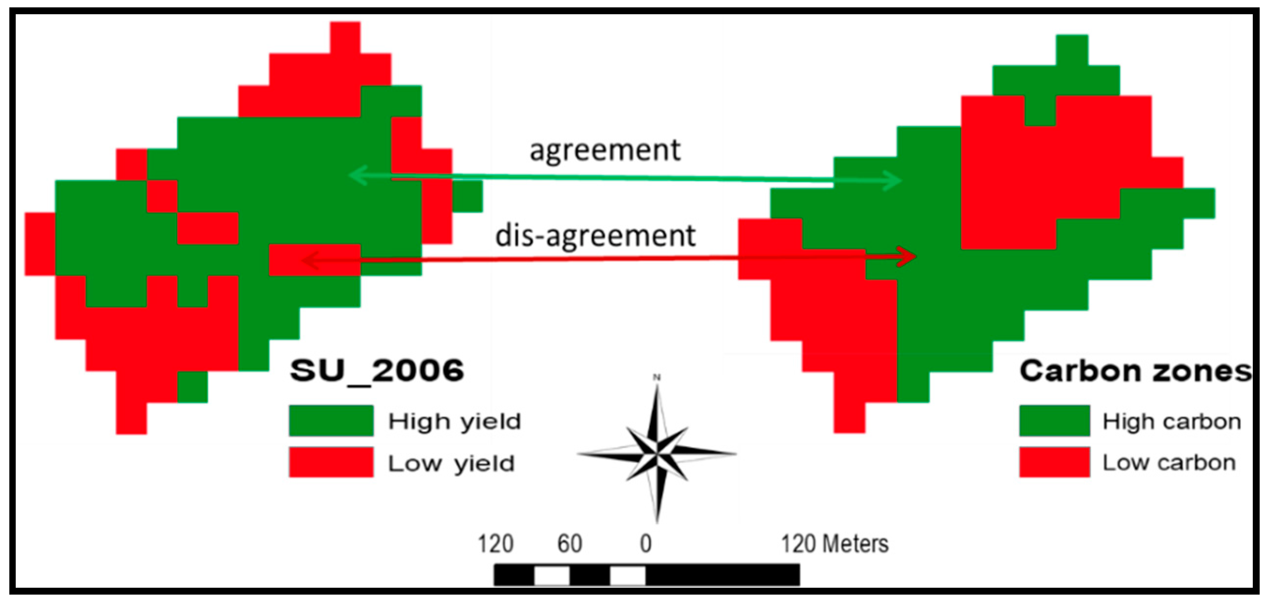
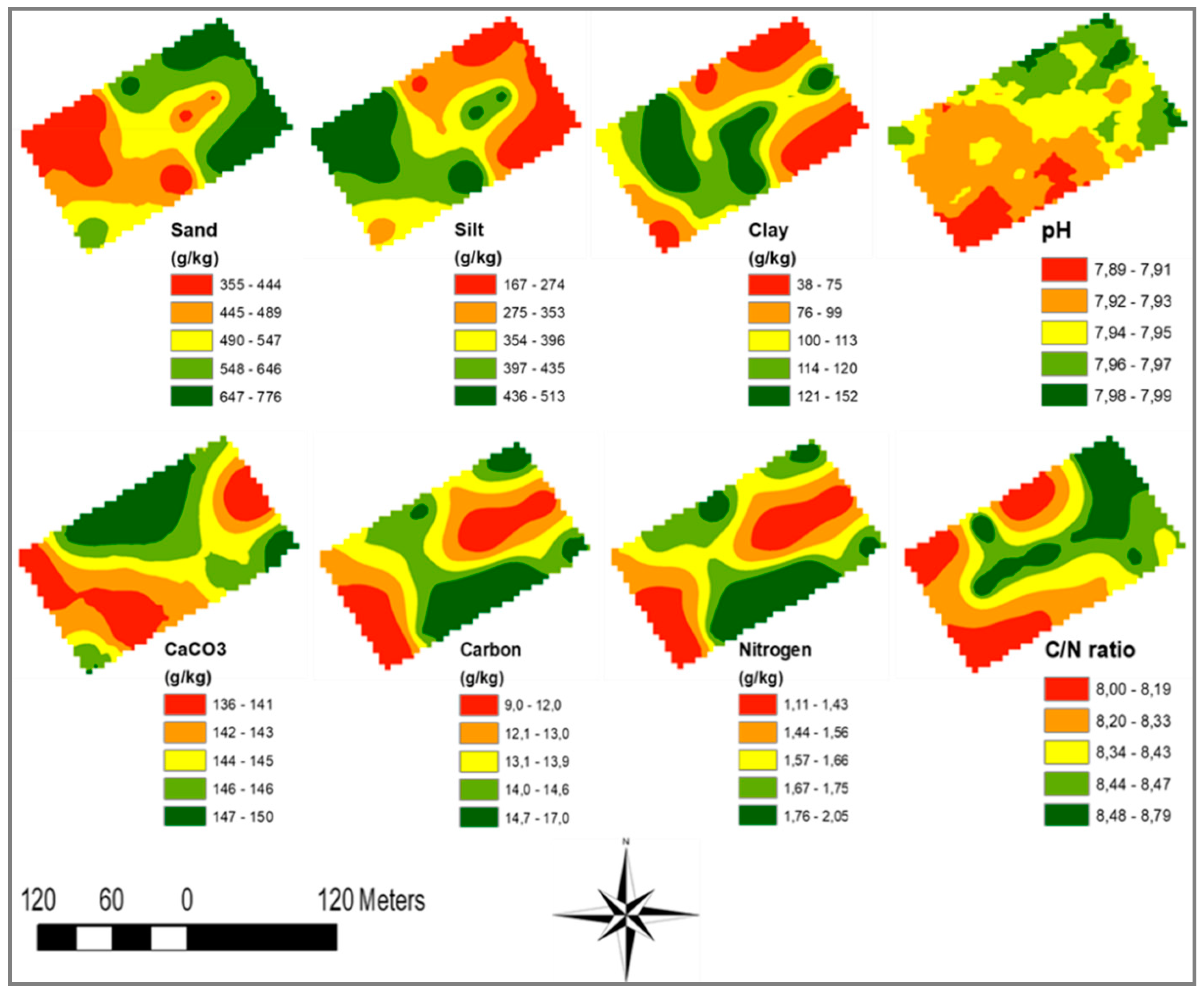
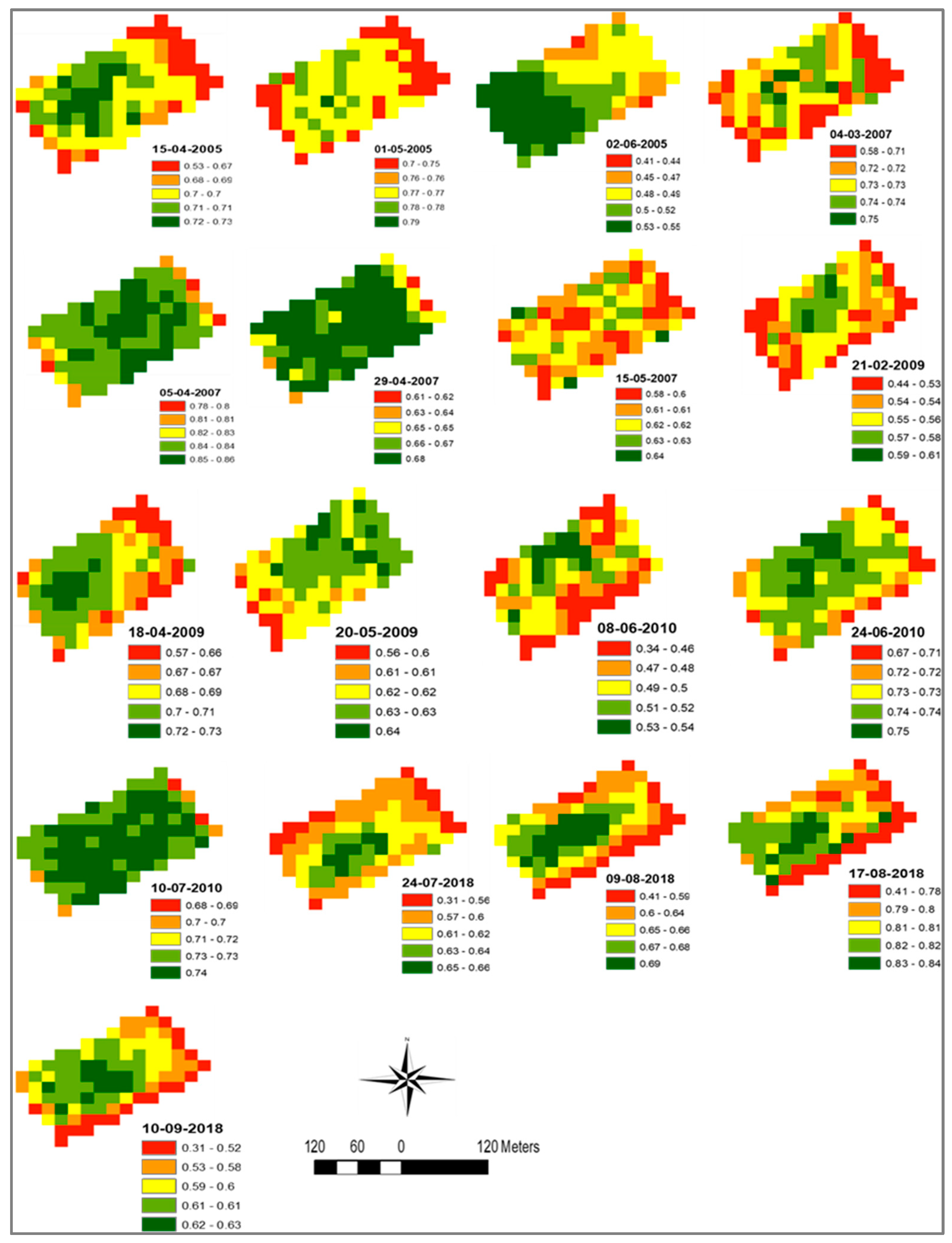
In this respect, it is evidenced that the two-zone maps of soil properties, NDVI values, and multiple yields (Figure 6 and Figure 7) have pixels of sufficient size (30 m) for dose variations to be implemented when passing from the low to the high zone, and vice versa. This is associated with modest patchiness of the two-zone maps (Figure 6 and Figure 7): only some single NDVI maps (e.g., 24-06-2010 in Figure 6) denote a patchy distribution that could pose problems in the differential application of some factor doses. However, the multiple soil and NDVI map (Figure 7) was not affected by this drawback, as the eight single parameters contributing to the multiple soil and NDVI maps provided the buffering that is a desired characteristic in a map intended for future use. The multiple yield two-zone map (
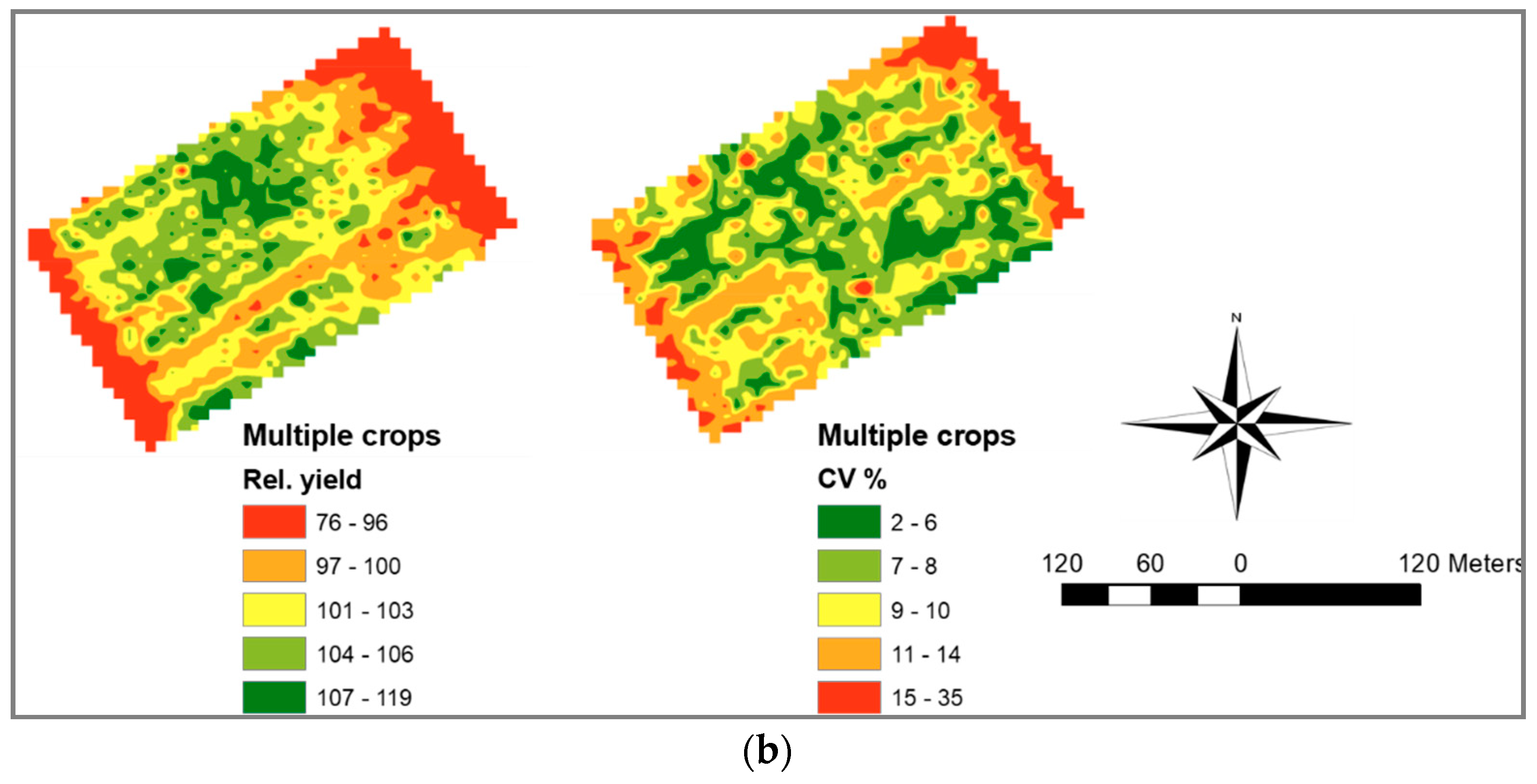
Figure 7) is an equally well-buffered map, as it originates from the multiple crops relative yield map (Figure 3b). The good agreement between the multiple soil and NDVI map, and multiple yield map (83% in Table 13), is a good premise for differential management of soil- and NDVI-based two zones in future cropping seasons.

5. Conclusions

Arable crop fields subjected for a number of years to georeferenced yield mapping obtain an amount of data deserving to be exploited in future crop management. The present work outlines a way to use these data in a field case study, by combining a temporal series of yield data from different crops into a standardized average yield, mapped through the field. This represents a robust indication of field spatial variability across varying weather and crop conditions. In parallel to this, spectral vegetation indices from remote sources and soil analyses could be obtained, and the soil and spectral vegetation data best correlated with yield could be combined into a multiple parameter mapped through the field. Geostatistical and clustering techniques were proven to be able to establish a suitable number of management zones across the field; in this case, it was only two zones, owing to the modest yield variability in the surveyed field. Lastly, a good agreement in the high and low zone between the multiple soil and spectral vegetation and multiple yield map, in this case 83 pixels out of 99 with agreement, is the ultimate proof that is needed to support the use of the soil- and vegetational-index-based map in the management of subsequent crops.

Supplementary Materials

The following supporting information can be downloaded at: https://www.mdpi.com/article/10.3390/agriculture12020231/s1. Table S1: Weather conditions during the seven crop growing seasons; Figure S1: Semi-variogram model of standardized crop yields; Table S2: Descriptive statistics of soil traits; Figure S2: Semi-variogram models of NDVI data; Figure S3: Single soil property zones; Figure S4: Single NDVI zones; Table S3: Statistical differences between 2-zone single soil property maps and their pixel agreements with yield zones; Table S4: Statistical differences between 2-zone single NDVI maps and their pixel agreements with yield zones; Figure S5: Semi-variogram graph of soil traits.

Author Contributions

Conceptualization, A.A., R.M. and L.B.; methodology, A.A., V.R., R.M., F.L. and L.B.; validation, V.R., G.F. and L.B.; formal analysis, A.A., R.M. and F.L.; investigation, G.F.; data curation, A.A., G.F. and L.B.; writing—original draft preparation, A.A. and L.B.; writing—review and editing, R.M., F.L. and L.B.; critically revising, A.A., V.R., R.M., G.F., F.L. and L.B.; supervision, V.R., R.M. and L.B.; funding acquisition, V.R.; final approval, A.A., V.R., R.M., G.F., F.L. and L.B. All authors have read and agreed to the published version of the manuscript.

Funding

This research received no external funding.

Institutional Review Board Statement

Not relevant to this study.

Informed Consent Statement

Not relevant to this study.

Data Availability Statement

Publicly available datasets were analyzed in this study. This data can be found here: [https://earthexplorer.usgs.gov/] (accessed on 30 December 2021).

Conflicts of Interest

The authors declare no conflict of interest.

References

  1. Khosla, R.; Fleming, K.; Delgado, J.A.; Shaver, T.M.; Westfall, D.G. Use of site specific management zones to improve nitrogen management for precision agriculture. J. Soil Water Conserv. 2002, 57, 513–518. [Google Scholar]
  2. Schepers, A.R.; Shanahan, J.F.; Liebig, M.K.; Schepers, J.S.; Johnson, S.H.; Luchiari, A., Jr. Appropriateness of management zones for characterizing spatial variability of soil properties and irrigated corn yields across years. Agron. J. 2004, 96, 195–203. [Google Scholar] [CrossRef] [Green Version]
  3. Fleming, K.L.; Westfall, D.G.; Wiens, D.W.; Brodah, M.C. Evaluating farmer developed management zone maps for variable rate fertilizer application. Precis. Agric. 2000, 2, 201–215. [Google Scholar] [CrossRef]
  4. Basso, B.; Ritchie, J.T.; Cammarano, D.; Sartori, L. A strategic and tactical management approach to select optimal N fertilizer rates for wheat in a spatially variable field. Eur. J. Agron. 2011, 35, 215–222. [Google Scholar] [CrossRef]
  5. Bao-wei, S.; Geng-xing, Z.; Chao, D. Spatio-temporal variability of soil nutrients and the responses of growth during growth stages of winter wheat in the north of China. PLoS ONE 2018, 13, e398701. [Google Scholar]
  6. Page, T.; Haygarth, P.M.; Beven, K.J.; Jones, A.; Butler, T.; Keeler, C.; Freer, J.; Owens, P.N.; Wood, G.A. The spatial variability of soil phosphorus in relation to topographic indices and important source areas: Samples to assess the risks to water quality. J. Environ. Qual. 2005, 34, 2263–2277. [Google Scholar] [CrossRef] [PubMed] [Green Version]
  7. Rufo, M.L.; Bollero, G.A.; Hoeft, R.G.; Bullock, D.G. Spatial variability of the Illinois soil nitrogen test: Implications for soil sampling. Agron. J. 2005, 97, 1485–1492. [Google Scholar] [CrossRef]
  8. Oshunsanya, S.O.; Oluwasemire, K.O.; Taiwo, O.J. Use of GIS to delineate sitespecific management zone for precision agriculture. Commun. Soil Sci. Plant Anal. 2017, 48, 565–575. [Google Scholar] [CrossRef]
  9. Peralta, N.R.; Costa, J.L. Delineation of management zones with soil apparent electrical conductivity to improve nutrient management. Comput. Electron. Agric. 2013, 99, 218–226. [Google Scholar] [CrossRef] [Green Version]
  10. Chatterjee, S.; Santra, P.; Majumdar, K.; Ghosh, D.; Das, I.; Sanyal, S.K. Geostatistical approach for management of soil nutrients with special emphasis on different forms of potassium considering their spatial variation in intensive cropping system of West Bengal, India. Environ. Monit. Assess. 2015, 187, 1–17. [Google Scholar] [CrossRef]
  11. Goovaerts, P. Geostatistical tools for characterizing the spatial variability of microbiological and physico-chemical soil properties. Biol. Fertil. Soils 1998, 27, 315–334. [Google Scholar] [CrossRef] [Green Version]
  12. Boydell, B.; McBratney, A.B. Identifying potential within field management zones from cotton yield estimates. In Proceedings of the 2nd European Conference on Precision Agriculture, Odense, Denmark, 11–15 July 1999; pp. 331–341. [Google Scholar]
  13. Jaynes, D.B.; Kaspar, T.C.; Colvin, T.S.; James, D.E. Cluster analysis of spatiotemporal corn yield patterns in an Iowa field. Agron. J. 2003, 95, 574–586. [Google Scholar] [CrossRef]
  14. Ali, A.; Martelli, R.; Scudiero, E.; Lupia, F.; Falsone, G.; Rondelli, V.; Barbanti, L. Soil and climate factors drive spatio-temporal variability of arable crop yields under uniform management in Northern Italy. Arch. Agron. Soil Sci. 2021, 1–15. [Google Scholar] [CrossRef]
  15. Corwin, D.L.; Lesch, S.M.; Shouse, P.J.; Soppe, R.; Ayars, J.E. Identifying soil properties that influence cotton yield using soil sampling directed by apparent soil electrical conductivity. Agron. J. 2003, 95, 352–364. [Google Scholar] [CrossRef] [Green Version]
  16. Huang, S.W.; Jing, J.Y.; Yang, L.P.; Cheng, M.F. Spatial variability and regionalized management of soil nutrients in the grain crop region in Yutian County. Acta Pedol. Sin. 2003, 40, 79–88. (In Chinese) [Google Scholar]
  17. Johnson, C.K.; Doran, J.W.; Duke, H.R.; Wienhold, B.J.; Eskridge, K.M.; Shanahan, J.F. Field-scale electrical conductivity mapping for delineating soil condition. Soil Sci. Soc. Am. J. 2001, 65, 1829–1837. [Google Scholar] [CrossRef] [Green Version]
  18. Long, D.S.; Carlson, G.R.; DeGloria, S.D. Quality of field management maps. In Proceedings of the 2nd International Conference on Site-Specific Management for Agricultural Systems, Minneapolis, MN, USA, 27–30 March 1994; pp. 251–271. [Google Scholar]
  19. Stafford, J.V.; Lark, R.M.; Bolam, H.C. Using yield maps to regionalize fields into potential management units. In Proceedings of the Fourth International Conference on Precision Agriculture, Madison, WI, USA, 19–22 July 1998; pp. 225–237. [Google Scholar]
  20. Hansen, P.M.; Schjoerring, J.K. Reflectance measurement of canopy biomass and nitrogen status in wheat crops using normalized difference vegetation indices and partial least squares regression. Remote Sens. Environ. 2003, 86, 542–553. [Google Scholar] [CrossRef]
  21. El Nahry, A.H.; Ali, R.R.; El Baroudy, A.A. An approach for precision farming under pivot irrigation system using remote sensing and GIS techniques. Agric. Water Manag. 2011, 98, 517–531. [Google Scholar] [CrossRef]
  22. Ferguson, R.B.; Lark, R.M.; Slater, G.P. Approaches to management zone definition for use of nitrification inhibitors. Soil Sci. Soc. Am. J. 2003, 67, 937–947. [Google Scholar] [CrossRef]
  23. Corwin, D.L.; Plant, R.E. Applications of apparent soil electrical conductivity in precision agriculture. Comput. Electron. Agric. 2005, 46, 1–10. [Google Scholar] [CrossRef]
  24. Moral, F.J.; Terrón, J.M.; Da Silva, J.M. Delineation of management zones using mobile measurements of soil apparent electrical conductivity and multivariate geostatistical techniques. Soil Tillage Res. 2010, 106, 335–343. [Google Scholar] [CrossRef]
  25. Doerge, T. Defining management zones for precision farming. Crop. Insights 1999, 8, 1–5. [Google Scholar]
  26. Guastaferro, F.; Castrignanò, A.; De Benedetto, D.; Sollitto, D.; Troccoli, A.; Cafarelli, B. A comparison of different algorithms for the delineation of management zones. Precis. Agric. 2010, 11, 600–620. [Google Scholar] [CrossRef]
  27. Fraisse, C.W.; Sudduth, K.A.; Kitchen, N.R. Delineation of site-specific management zones by unsupervised classification of topographic attributes and soil electrical conductivity. Trans. ASAE 2001, 44, 155–166. [Google Scholar] [CrossRef] [Green Version]
  28. Franzen, D.W.; Kitchen, N.R. Developing management zones to target nitrogen applications. SSMG-5. In Site-Specific Management Guidelines Series; Potash & Phosphate Institute: Singapore, 1999. [Google Scholar]
  29. Franzen, D.W.; Hopkins, D.H.; Sweeney, M.D.; Ulmer, M.K.; Halvorson, A.D. Evaluation of soil survey scale for zone development of site-specific nitrogen management. Agron. J. 2002, 94, 381–389. [Google Scholar]
  30. Kyaw, T.; Ferguson, R.B.; Adamchuk, V.I.; Marx, D.B.; Tarkalson, D.D.; McCallister, D.L. Delineating site-specific management zones for pH-induced iron chlorosis. Precis. Agric. 2008, 9, 71–84. [Google Scholar] [CrossRef] [Green Version]
  31. Metzger, M.J.; Bunce, R.G.H.; Jongman, R.H.; Mücher, C.A.; Watkins, J.W. A climatic stratification of the environment of Europe. Glob. Ecol. Biogeogr. 2005, 14, 549–563. [Google Scholar] [CrossRef]
  32. Ali, A.; Martelli, R.; Lupia, F.; Barbanti, L. Assessing multiple years’ spatial variability of crop yields using satellite vegetation indices. Remote Sens. 2019, 11, 2384. [Google Scholar] [CrossRef] [Green Version]
  33. Gee, G.W.; Bauder, J.W. Particle-size analysis. In Methods of Soil Analysis, 2nd ed.; Klute, A., Ed.; Part 1. Agron. Monogr. 9; ASA and SSSA: Madison, WI, USA, 1986; pp. 383–411. [Google Scholar]
  34. Loeppert, R.H.; Suarez, D.L. Carbonate and gypsum. In Methods of Soil Analysis; Part 3. Chemical Methods; SSSA-Book Series no. 5; Soil Science Society of America, Ins., American Society of Agronomy: Madison, WI, USA, 1996; pp. 437–474. [Google Scholar]
  35. Cambardella, C.A.; Moorman, T.B.; Parkin, T.B.; Karlen, D.L.; Novak, J.M.; Turco, R.F.; Konopka, A.E. Field-scale variability of soil properties in central Iowa soils. Soil Sci. Soc. Am. J. 1994, 58, 1501–1511. [Google Scholar] [CrossRef]
  36. Xiao, Y.; Gu, X.; Yin, S.; Shao, J.; Cui, Y.; Zhang, Q.; Niu, Y. Geostatistical interpolation model selection based on ArcGIS and spatio-temporal variability analysis of groundwater level in piedmont plains, northwest China. SpringerPlus 2016, 5, 425. [Google Scholar] [CrossRef] [Green Version]
  37. Blackmore, S. The interpretation of trends from multiple yield maps. Comput. Electron. Agric. 2000, 26, 37–51. [Google Scholar] [CrossRef]
  38. Fridgen, J.J.; Kitchen, N.R.; Sudduth, K.A.; Drummond, S.T.; Wiebold, W.J.; Fraisse, C.W. Management Zone Analyst (MZA) Software for Subfield Management Zone Delineation. Agron. J. 2004, 96, 100–108. [Google Scholar]
  39. Allen, R.G.; Pereira, L.S.; Raes, D.; Smith, M. Crop Evapotranspiration-Guidelines for Computing Crop Water Requirements-FAO Irrigation and Drainage; Report No.: 56; D05109.; FAO: Rome, Italy, 1998. [Google Scholar]
  40. Da Silva, J.M. Analysis of the spatial and temporal variability of irrigated maize yield. Biosyst. Eng. 2006, 94, 337–349. [Google Scholar] [CrossRef] [Green Version]
  41. Scudiero, E.; Teatini, P.; Manoli, G.; Braga, F.; Skaggs, T.; Morari, F. Workflow to establish time-specific zones in precision agriculture by spatiotemporal integration of plant and soil sensing data. Agronomy 2018, 8, 253. [Google Scholar] [CrossRef] [Green Version]
  42. Jiang, G.P.; Grafton, M.; Pearson, D.; Bretherton, M.; Holmes, A. Predicting spatiotemporal yield variability to aid arable precision agriculture in New Zealand: A case study of maize-grain crop production in the Waikato region. N. Z. J. Crop. Hortic. Sci. 2021, 49, 41–62. [Google Scholar] [CrossRef]
  43. Chang, J.Y.; Clay, D.E.; Carlson, C.G.; Reese, C.L.; Clay, S.A.; Ellsbury, M.M. Defining yield goals and management zones to minimize yield and nitrogen and phosphorus fertilizer recommendation errors. Agron. J. 2004, 96, 825–831. [Google Scholar] [CrossRef] [Green Version]
  44. McEntee, P.J.; Bennett, S.J.; Belford, R.K. Mapping the spatial and temporal stability of production in mixed farming systems: An index that integrates crop and pasture productivity to assist in the management of variability. Precis. Agric. 2020, 21, 77–106. [Google Scholar] [CrossRef]
  45. Kerry, R.; Oliver, M.A. Average variograms to guide soil sampling. Int. J. App. Earth Obs. Geoinf. 2004, 5, 307–325. [Google Scholar] [CrossRef]
  46. Kerry, R.; Oliver, M.A. Determining nugget: Sill ratios of standardized variograms from aerial photographs to krige sparse soil data. Precis. Agric. 2008, 9, 33–56. [Google Scholar] [CrossRef]
  47. McBratney, A.Á.; Pringle, M.J. Estimating average and proportional variograms of soil properties and their potential use in precision agriculture. Precis. Agric. 1999, 1, 125–152. [Google Scholar] [CrossRef]
Figure 1. Study site and soil sampling points across the field located in Northern Italy.
Agriculture 12 00231 g001
Figure 2. Example of pixel agreement for the calculation of pixel similarity.
Agriculture 12 00231 g002
Figure 3. Spatial maps (n = 937) of single crop yields (a), and multiple crop yields and the related coefficient of variation (CV) (b).
Agriculture 12 00231 g003aAgriculture 12 00231 g003b
Figure 4. Spatial variability of soil traits (n = 937).
Agriculture 12 00231 g004
Figure 5. Spatial variability maps of NDVI indices (n = 99).
Agriculture 12 00231 g005
Figure 6. Two-zone maps of single soil properties and NDVI indices (these latter simply indicated by their acquisition dates).
Agriculture 12 00231 g006
Figure 7. Two-zone multiple soil and NDVI map, (a); two-zone multiple crops yield map (b).
Agriculture 12 00231 g007
Table 1. Seeding and harvesting dates, and crop duration of cultivated crops.
Crop & YearBotanical NameSeedingHarvestingDuration (Days)
BW 2005Triticum aestivum L.19 October (2004)24 June248
SU 2006Helianthus annuus L.10 April12 September155
BW 2007Triticum aestivum L.9 October (2006)18 June252
BW 2009Triticum aestivum L.21-October (2008)30 June252
SO 2010Sorghum bicolor L.21 April28 August129
MA 2018Zea mays L.18 June25 September99
MA 2020Zea mays L.28 March8 August133
BW, bread wheat; SU, sunflower; SO, sorghum; MA, maize.
Table 2. Prospection of remotely sensed NDVI imagery and corresponding dates after sowing (DAS).
Crop &
Year
LS-
Mission
DateDAS
BW 2005LS-7 ETM+15 April178
LS-5 TM23 April186
LS-7 ETM+1 May194
LS-7 ETM+2 June226
SU 2006LS-5 TM26 April16
15 July96
31 July112
16 August127
BW 2007LS-7 ETM+4 March146
LS-7 ETM+5 April178
LS-5 TM29 April202
LS-5 TM15 May218
BW 2009LS-7 ETM+21 February123
LS-5 TM18 April179
LS-5 TM20 May211
SO 2010LS-5 TM8 June48
24 June64
10 July80
MA 2018LS-7 ETM+24 July36
LS-7 ETM+9 August52
LS-8 OLI17 August60
LS-7 ETM+10 September84
MA 2020LS-7 ETM+26 May59
LS-8 OLI19 June83
LS-8 OLI5 July99
LS-8 OLI21 July115
BW, bread wheat; SU, sunflower; SO, sorghum; MA, maize; LS, Landsat; DAS, days after sowing.
Table 3. Values of FPI and NCE based on standardized crop yields over seven years for the delineation of 2, 3, and 4 zones.
Number of ClustersCrop Yields
FPINCE
20.03690.0151
30.10070.0536
40.13420.0809
FPI (fuzziness performance index), NCE (normalized classification entropy).
Table 4. Descriptive statistics of standardized crop yields over seven years (means = 100).
SourceMedianMinMaxSDSkewnessKurtosis
BW_20051024312512.6−1.232.84
SU_20061004614714−0.110.56
BW_20071015714012.8−0.450.69
BW_20091025213312.9−0.80.75
SO_20101006620810.41.2112.5
MA_2018101791074.4−1.533.21
MA_20201012914912.6−0.882.38
Actual mean yield (t/ha); BW_2005 (6.91), SU_2006 (2.00), BW_2007 (3.50), BW_2009 (6.59), SO_2010 (2.71), MA_2018 (14.52), MA_2020 (24.5); BW, bread wheat; SU, sunflower; SO, sorghum; MA, maize; SD, standard deviation.
Table 5. Semi-variogram parameters of standardized crop yields over seven years.
SourceModelC0C0 + Ca (m)C0/(C0 + C) %SpDR2MAERMSEASE
BW_2005Stable27.81402920S0.960.0289.7510.5
SU_2006Stable40.633014612S0.95−0.003510.112.5
BW_2007Stable0283520S0.900.006110.712.3
BW_2009Spherical24.81641015S0.940.0217.877.78
SO_2010Stable0212870S0.920.0986.6910.3
MA_2018Exp.013250S0.870.00041.461.92
MA_2020Stable30.71892216S0.87−0.086.817.56
BW, bread wheat; SU, sunflower; SO, sorghum; MA, maize; C0, nugget; C, partial sill; C0 + C, sill; a, range; C0/(C0 + C), nugget-to-sill ratio; SpD, spatial dependence; S, strong; R2, coefficient of determinants, MAE, mean absolute error; RMSE, root mean square error; ASE, absolute standard error.
Table 6. Descriptive statistics of soil traits (depth 0–0.6 m).
Soil VariablesMeanMedianMinMaxSDSkewnessKurtosis
Sand (g/kg)5495043357931470.22−1.32
Silt (g/kg)354379153529116−0.16−1.33
Clay (g/kg)971103515637.9−0.28−1.39
pH7.937.907.728.190.130.72−0.1
CaCO3 (g/kg)14414511616211.1−0.710.66
C (g/kg)13.514.08.717.12.33−0.4−0.54
N (g/kg)1.621.681.082.060.28−0.32−0.7
C:N8.348.407.968.810.230.07−0.85
ECe (ds/m)0.420.410.260.630.10.6−0.39
Min, minimum; Max, maximum; SD, standard deviation.
Table 7. Semi-variogram parameters of soil traits.
SourceModelC0C0 + Ca (m)C0/(C0 + C)%SpDR2MAERMSEASE
SandSpherical07171190S0.981.1612.2915.48
SiltExp.05311250S0.96−0.7812.2217.06
ClayExp.039.51200S0.95−0.203.834.73
pHExp.00.00003900S0.92−0.000110.00420.0045
CaCO3Exp.00.481390S0.96−0.0120.400.49
CExp.00.161180S0.940.00340.260.30
NExp.00.00241300S0.940.000920.0320.036
C:NSpherical00.00351400S0.94−0.00200.0260.031
C0, nugget; C, partial sill; C0 + C, sill; a, range; C0/(C0 + C), nugget-to-sill ratio; SpD, spatial dependence; S, strong; R2, coefficient of determinants, MAE, mean absolute error; RMSE, root mean square error; ASE, absolute standard error.
Table 8. Pearson’s correlations between soil traits and crop yields (n = 99).
Soil TraitsBW_2005SU_2006BW_2007BW_2009SO_2010MA_2018MA_2020Mean Yields
Sand−0.69−0.09−0.19−0.17−0.08−0.58−0.07−0.44
Silt0.670.080.200.140.080.590.070.43
Clay0.710.230.170.340.040.370.100.47
pH−0.680.15−0.08−0.060.16−0.530.24−0.26
CaCO3−0.180.290.380.370.640.140.430.36
Carbon0.090.120.440.250.170.070.610.30
Nitrogen0.150.110.470.230.200.160.600.34
C/N−0.400.10−0.120.15−0.16−0.560.08−0.22
ECe−0.010.100.360.170.10−0.040.480.18
BW, bread wheat; SU, sunflower; SO, sorghum; MA, maize; bold letter correlations are significant at p < 0.05 according to Pearson correlation.
Table 9. Descriptive analysis of NDVI indices.
Crop & YearAcquisition DateMeanMedianMinMaxSDSkewnessKurtosis
BW 200515 April0.690.700.530.730.03−2.227.67
23 April0.470.490.220.520.06−2.616.19
1 May0.760.760.70.790.02−1.331.5
2 June0.50.500.410.550.03−0.42−0.81
SU 200626 April0.160.160.130.280.032.045.01
15 July0.550.560.470.610.03−0.40.51
31 July0.410.410.330.450.02−0.961.12
16 August0.320.330.10.570.130.01−1.25
BW 20074 March0.720.730.580.750.03−2.356.31
5 April0.840.840.780.860.02−1.733.29
29 April0.670.670.610.680.01−1.763.55
15 May0.610.610.580.640.01−0.47−0.02
BW 200921 February0.540.550.440.610.03−0.821.81
18 April0.680.670.570.730.03−1.184.13
20 May0.610.620.560.640.01−1.775.34
SO 20108 June0.480.490.340.540.04−1.141.79
24 June0.720.730.670.750.01−1.462.58
10 July0.720.730.680.740.01−2.478.54
MA 201824 July0.590.600.310.660.06−2.7510.09
9 August0.640.650.410.690.05−1.392.49
17 August0.780.810.410.840.07−2.67.72
10 September0.560.590.310.630.07−1.863.05
MA 202026 May0.550.580.30.650.08−1.551.67
19 June0.840.880.370.90.11−2.938
5 July0.810.850.370.870.11−2.757.13
21 July0.80.830.40.850.09−2.847.64
BW, bread wheat; SU, sunflower; SO, sorghum; MA, maize; Min, minimum; Max, maximum; SD, standard deviation.
Table 10. Pearson’s correlations (r values) between NDVI data in different acquisition dates and crop yields (n = 99).
BW_2005SU_2006BW_2007BW_2009SO_2010MA_2018MA_2020
0.79 (15 April)−0.30 (26 April)0.53 (4 March)0.79 (21 February)0.29 (8 June)0.55 (24 July)0.16 (26 May)
0.05 (23 April)−0.17 (15 July)0.57 (5 April)0.48 (19 April)0.53 (24 June)0.36 (9 August)0.18 (19 June)
0.71 (1 May)0.06 (31 July)0.58 (29 April)0.54 (20 May)0.31 (10 July)0.32 (17 August)0.20 (5 July)
0.58 (2 June)0.18 (16 August)0.31 (15 May) 0.24 (10 September)0.22 (21 July)
BW, bread wheat; SU, sunflower; SO, sorghum; MA, maize; correlations in bold are significant at p < 0.05.
Table 11. Semi-variogram analysis of NDVI index and best fit exponential model performance.
CropAcquisition DateC0C0 + Ca (m)C0/(C0 + C) %SpDR2MAERMSEASE
BW 200515 April00.87660S0.990.0010.0170.012
1 May0.581.0113157M0.850.000490.0120.0098
2 June01.141020S0.900.00020.010.01
BW 20074 March0.130.946914S0.980.000860.0170.015
5 April0.0051.01780S0.970.000690.00980.0085
29 April01.01820S0.960.000560.010.0089
15 May01.11920S0.950.000020.0110.01
BW 200921 February01.03560S0.980.00070.0170.014
18 April01.11920S0.980.000030.0110.0102
20 May0.570.965659M0.870.000150.00830.0071
SO 20108 June01.21020S0.990.000060.020.0201
24 June0.360.925639M0.880.000560.010.0081
10 July0.610.925967M0.650.00030.00860.0069
MA 201824 July01.091300S0.990.00240.0310.023
9 August01.011100S0.990.0010.0190.016
17 August0.1218312S0.990.00330.0380.029
10 September00.95630S0.990.00190.0260.022
BW, bread wheat; SU, sunflower; SO, sorghum; MA, maize; C0, nugget; C, partial sill; C0 + C, sill; a, range; C0/(C0 + C), nugget-to-sill ratio; SpD, spatial dependence; S, strong; M, moderate; R2, coefficient of determinants, MAE, mean absolute error; RMSE, root mean square error; ASE, absolute standard error.
Table 12. Statistical differences between two-zone single soil properties and NDVI indices, and their pixel agreements (percentage) with two-zone multiple crops yield map.
VariablesZonesData
Points
Mean ± SDAgreement
(%)
Clay (g/kg)High clay
Low clay
67112 ±7.39 a94
3279.3 ± 10.42 b
CaCO3 (g/kg)High CaCO349146 ± 1.31 a76
Low CaCO350142 ± 1.05 b
Nitrogen (g/kg)High Nitrogen541.69 ± 0.08 a81
Low Nitrogen451.48 ± 0.07 b
NDVI 15-Apr-2005High NDVI780.70 ± 0.012 a95
Low NDVI210.65 ± 0.032 b
NDVI 29-Apr-2007High NDVI840.67 ± 0.006 a89
Low NDVI150.64 ± 0.013 b
NDVI 21-Feb-2009High NDVI500.57 ± 0.014 a77
Low NDVI490.52 ± 0.021 b
NDVI 24-Jun-2010High NDVI510.73 ± 0.004 a78
Low NDVI480.71 ± 0.013 b
NDVI 24-Jul-2018High NDVI950.60 ± 0.033 a78
Low NDVI40.38 ± 0.068 b
SD, standard deviation; means bearing different letters are significantly different within 2-zone classes at p < 0.05 according to the least-significant difference (LSD) test.
Table 13. Statistical differences between two-zone multiple soil properties and NDVI indices, and their pixel agreements (percentage) with two-zone multiple crops yield map.
VariablesZonesData
Points
Mean ± SDAgreement (%)
Clay (g/kg)High values89103 ± 16.7 a83%
Low values1087.5 ± 19.8 b
CaCO3 (g/kg)High values89144 ± 2.09 a
Low values10143 ± 2.53 a
Nitrogen (g/kg)High values891.61 ± 0.13 a
Low values101.54 ± 0.14 a
NDVI 15-Apr-05High values890.70 ± 0.02 a
Low values100.63 ± 0.04 b
NDVI 29-Apr-07High values890.67 ± 0.01 a
Low values100.63 ± 0.01 b
NDVI 21-Feb-09High values890.55 ± 0.02 a
Low values100.50 ± 0.03 b
NDVI 24-Jun-10High values890.73 ± 0.01 a
Low values100.69 ± 0.01 b
NDVI 24-Jul-18High values890.60 ± 0.03 a
Low values100.47 ± 0.09 b
Multiple crops yield (%)High73102 ± 1.72 a
Low2694 ± 3.08 b
SD, standard deviation; means bearing different letters are significantly different within 2-zone classes at p < 0.05 according to the least-significant difference (LSD) test.
Publisher’s Note: MDPI stays neutral with regard to jurisdictional claims in published maps and institutional affiliations.

