Artificial Intelligence-Based Real-Time Pineapple Quality Classification Using Acoustic Spectroscopy

Abstract

The pineapple is an essential fruit in Taiwan. Farmers separate pineapples into two types, according to the percentages of water in the pineapples. One is the “drum sound pineapple” and the other is the “meat sound pineapple”. As there is more water in the meat sound pineapple, the meat sound pineapple more easily rots and is more challenging to store than the drum sound pineapple. Thus, farmers need to filter out the meat sound pineapple, so that they can sell pineapples overseas. The classification, based on striking the pineapple fruit with rigid objects (e.g., plastic rulers) is most commonly used by farmers due to the negligibly low costs and availability. However, it is a time-consuming job, so we propose a method to automatically classify pineapples in this work. Using embedded onboard computing processors, servo, and an ultrasonic sensor, we built a hitting machine and combined it with a conveyor to automatically separate pineapples. To classify pineapples, we proposed a method related to acoustic spectrogram spectroscopy, which uses acoustic data to generate spectrograms. In the acoustic data collection step, we used the hitting machine mentioned before and collected many groups of data with different factors; some groups also included the noise in the farm. With these differences, we tested our deep learning-based convolutional neural network (CNN) performances. The best accuracy of the developed CNN model is 0.97 for data Group V. The proposed hitting machine and the CNN model can assist in the classification of pineapple fruits with high accuracy and time efficiency.

1. Introduction and Motivation

1.1. Introduction

The pineapple is an essential fruit in Taiwan [1]. Under the Taiwan Council of Agriculture, Executive Yuan, farmers planted 7819 hectares of pineapples and gained 407,822 metric tons in 2021 [2], which makes the pineapple the most abundant fruit in Taiwan. There are many varieties of pineapples, such as native pineapples, milk pineapples, and mango pineapples. Most pineapples are planted in southern Taiwan (e.g., in Nantou, JiaYi, Tainan, Gaoxiong, and Pingdong). Since pineapples are planted, farmers can harvest fruits after 18 months. If pineapples grow normally, they will mature between June and August; however, it is rainy during this season in Taiwan—the weather makes pineapples contain more water than expected. When pineapples contain too much water, they rot more easily. Farmers separate pineapples into two types, according to the percentages of water in the pineapples: one type is the “drum sound pineapple”, which contains less water, and the other is the “meat sound pineapple”, which contains more water. The drum sound pineapple looks light yellow. It has a sweet-and-sour taste, and it smells better. The meat sound pineapple looks dark yellow [3]. As the meat sound pineapple contains more water than the drum sound pineapple, it cannot be stored too long.

In Taiwan, most pineapples are sold overseas. To ship pineapples for a long time, farmers can only sell the drum sound pineapple; otherwise, pineapples would rot before they can be sold. The straightforward way to distinguish between the drum sound and the meat sound pineapples is by hitting the pineapple and listening to the sound [3], as Figure 1c shows. When hitting on the drum sound pineapple, it sounds like hitting on a drum, and when hitting on the meat sound pineapples, it sounds like hitting on an arm. Farmers would swing a ruler to hit the pineapples and listen to the sound. For each pineapple, farms need to hit pineapples more than three times to ensure the sound is a drum sound or meat sound. This procedure costs many human resources and machinery, as shown in Figure 1; thus, farmers need to hire many laborers who have good physical strength, because they need to classify huge quantities of pineapples via the sound test.

In the 1990s, the Taiwanese government set a goal to achieve agriculture automation [4]. With agriculture automation, the quality of agricultural products can be raised. There are many aspects of agriculture automation, such as automated planting machines, precise automated watering systems, environmental automated control systems, and automated quality and rank classifications of agricultural products. Recently, using automated rice machine systems in 50 exhibition centers, around 2 million Yuan (in operating costs) were saved for each phase of cultivation in one season. In the article’s conclusion [4], it was noted that agriculture automation is an area that combines the knowledge of agriculture as well as multi-disciplinary engineering and science.

1.2. Motivation and Contribution

Traditional pineapple classification methods are time- and resource-intensive processes and, thus, they increase processing costs. To help farmers classify pineapples efficiently, we propose an automatic pineapple classification machine. First, we designed a “hitting” machine combined with Raspberry Pi, servo, and an ultrasonic sensor. As a pineapple on the conveyor passes Raspberry Pi, notified by the ultrasonic sensor, it will trigger the servo to hit the pineapple. We used our hitting machine to collect sound data. We transformed the sound data from the amplitude/time domain to the frequency/time domain by a short-time Fourier transform to get the spectrogram. To classify pineapples by spectrogram, we built a convolutional neural network. We also collected data from different batches of pineapples in different conditions to test our model adaptability.

2. Related Works

Some methods present in the literature are used to automatically classify fruits and are used for different classification techniques. Some approaches use machine learning to learn farmers’ experiences, such as using acoustic data to classify fruits, while other approaches analyze the properties of the fruits, to find the differences between the different categories labeled by farmers.

Weangchai Kharamat et al. checked the ripeness of the durian via acoustic data [5]. The durians were separated into three categories, ripe, mid-ripe, and unripe. Using acoustic is the most common way to classify durians. The sound is made by sweeping rubber-tipped sticks on the durians. The authors collected data from 30 durians. They used a smartphone to record 0.3 s of audio. As for the smartphone settings: the sampling frequency was 16 kHz, with 16-bits mono audio. Finally, they obtained 300 data points for each category.

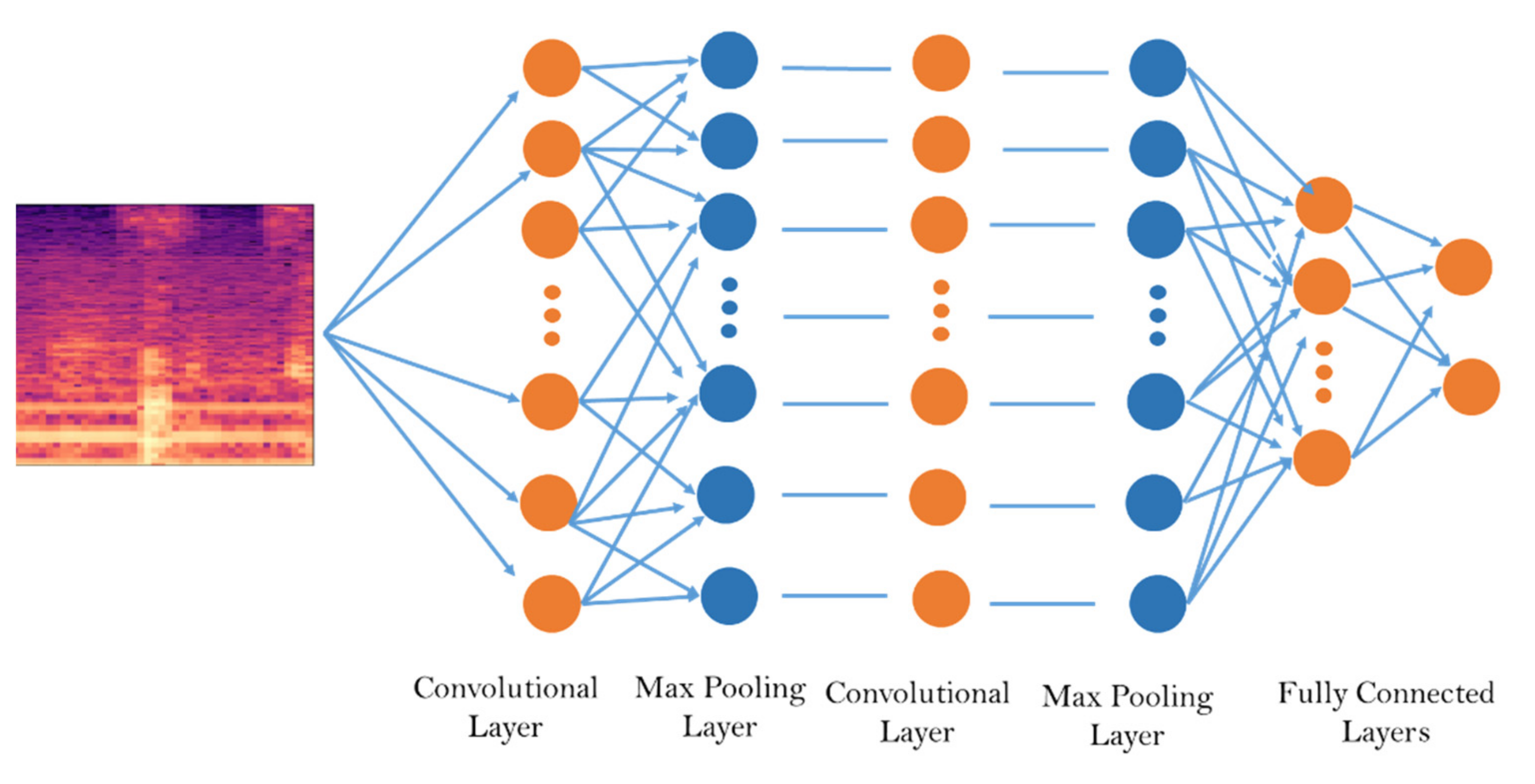
After collecting the data, the authors extracted the features by using Mel frequency cepstral coefficients (MFCCs) [6]. To get Mel frequency cepstral coefficients, there are four steps. First, use the Fourier transform to make the sound change to a frequency domain. Second, apply the triangular overlapping window and mapping to the Mel scale. Third, take the logs of power at each Mel frequency. Finally, transform the Mel log powers by a discrete cosine transform. The results of the Mel frequency cepstral coefficients are used as inputs of the convolutional neural network. The authors also applied a 25% dropout on layers two and four and a 50% dropout on the fully connected layer. The model was optimized by the Adam optimization algorithm. The model reached the highest testing accuracy, 0.89, with 150 epochs.

Arturo Baltazar et al. [7] classified tomatoes by the concept of data fusion. Data fusion [8] involves combining multiple data collected by different sensors. The authors collected three features of tomatoes—color, acoustic, and firmness. For color, they used a colorimeter; for acoustic, they designed a machine to hit tomatoes and record sound data. The firmness can be acquired by the nondestructive method if it is calculated by 2.1. S_c in the stiffness coefficient, f is the dominant frequency obtained from acoustic data, and m is the bulk mass of the fruit. The color and firmness data would be collected in specific intervals. Because the ranges of data are different, the authors used min–max normalization to limit the data in the range of 0 to 1 [9]. To classify tomatoes, the authors used a Bayesian classifier [10]. The classification error was reduced when the number of features rose.

Puneet Mishra et al. used near-infrared to analyze content in the pear [11]. Soluble solid content (SSC) and moisture content (MC) play an important role in fruit maturity and quality [12]. The authors used near-infrared to detect the content, which is a standard technology used in this field. The authors used the parameters of near-infrared in the spectral range of 310–1135 nm with a spectral resolution of 8–13 nm. They scanned at the bellies of the pears, calculating the average of six scans. To predict soluble solid content and moisture content, the authors used two common chemometric algorithms. One was interval partial least squares regression (iPLS2R) [13], which is used for predicting in a subset of continuous wavelengths, and the other was covariate selection (CovSel), which can select discrete wavelengths related to the content [14].

The authors also used model updating, which uses a few data from the new batch to improve the model. In the experiment, the authors selected 5, 10, and 20 samples by the Kennard–Stone (KS) sample partition technique from Batch 2 to recalibrate the model built from Batch 1. The Q2 of iPLS2R in soluble solid content improved from 0.71 to 0.76 with 5 and 10 samples; in moisture content, it improved from 0.84 to 0.87 with 20 samples. The Q2 of CovSel in soluble solid content improved from 0.73 to 0.77 with any number of sample selections; in moisture content, it improved from 0.84 to 0.85 with 5 and 20 samples.

R.P. Haff et al. used an X-ray to detect translucency in pineapples [15]. Translucency is a physiological disorder of pineapple. By using X-rays, the authors can get the internal image of a pineapple from the side. The pineapples were divided into five levels after cutting and examining the section. For the first level, there was no translucency in the pineapple. For the second level, there was less than 25% translucency. For the third level, there was 25–50% translucency. For the fourth level, there was 50–75% translucency. For the fifth level, there was more than 75% translucency. The first and second levels were considered good pineapples, and the others as bad. The X-ray pictures were used as the input of the logistic regression [16]. The output of the logistic regression was 1 and 0, which means the pineapples were good or bad. The R² of the model was 0.96.

Siwalak Pathaveer et al. [17] used multivariate data collected by nondestructive methods to analyze pineapple maturity and compared the results (i.e., with and without destructive methods). The non-destructive data were the specific gravity and acoustic impulses. The destructive data were flesh firmness (FF), soluble solid content (SSC), and titratable acidity (TA). The pineapples were separated into three classes—class A, Class B, and class C. Class A represented greater than 50% translucent yellow. Class B represented 25–50% translucent yellow. Class C represented less than 25% translucent yellow.

In the latest research from the Taiwan Agriculture Research Institute Council of Agriculture, Executive Yuan [18], the authors designed a product [19] that classified pineapples by resistance. They found that the difference between the drum sound pineapple and the meat sound pineapple might not be caused by the percentage of water, but by the distribution of water. As a result, using resistance to quantify the pineapple would be a better way than using capacitance. However, their product needs to be adjusted before being implemented in different batches.

The existing models in the literature can be improved in different ways. First, when using technology to analyze fruits, it should make the analysis accurate and help farmers reduce their work. Most previous works could not work automatically; some used high price devices. In this work, we designed an automatic classification machine that could distinguish between pineapple types and separate pineapples automatically, based on acoustic data. We also used our model to test different batches of pineapples collected in different conditions.

3. System Design and Implementation

We proposed a method to classify pineapples based on acoustic spectrogram spectroscopy. We designed a batting machine to hit pineapples and automatically collect the hitting sound for the acoustic data. After we obtained the audio data, we extracted important parts from the audio and augmented it. Finally, we built a convolutional neural network (CNN) [20].

The various components used in the development of this system are summarized in

Table 1. Components used in developing the system.

Components	Number
Raspberry Pi 4	1
Servo	1
Ultrasonic Sensor	1
Microphone	1
Conveyor	1

. Embedded onboard the computing processors, such as Raspberry Pi, Nvidia Jetson Nano was used to store and run the deep learning models, connect an ultrasonic sensor, a microphone, and a servo, as shown in Figure 2. The top and side views of the Raspberry installed on a conveyor belt are shown in the schematic diagram, Figure 3. The proposed system prototype developed in our lab is shown in Figure 4. The Raspberry Pi measures the distance across the conveyor that normally remains constant for the ultrasonic sensor, but the value of the distance would be smaller than the defined threshold when a pineapple passes the Raspberry Pi. Then the Raspberry Pi will open the microphone for 1 s, trigger the servo to hit the pineapple, send the acoustic data to the deep learning model to classify pineapples, and control the conveyor to separate the pineapple. The flowchart of the whole process is shown in Figure 5.

3.1. Data Collection and Preprocessing

To collect multiple data instances, we hit one pineapple multiple times and recorded it in one audio file. The automatic system was used to hit the pineapples to collect the test data similar to data that we obtained when we implemented the system. Figure 6 shows the flowchart of data collection, preprocessing, and data augmentation in the acoustic classification system.

Since we collected multiple “hit” sounds in one audio file, our goal was to extract them and create a new, strong, and clear sound for each hit sound. We used Librosa onset strength [21], calculating onset strength by spectral novelty functioning to find where the hit sound appeared. As we recorded k sounds in one audio file, the top-k onset strength was considered the hitting sounds. Onset was where the hit sound started, so we easily put the hit sound in the middle of 1 sec after we found the hit sound. This method can extract hitting sound perfectly if the audio is recorded in a stable environment; however, some data were collected in the farm factory, containing too many noises, such as humans talking, animals barking, and machines running, which were extracted due to their high “strengths”, and as they involved missing some “hit sounds”. As a result, we needed to listen to the one-second audio files to delete the audio with noise only.

3.1.1. Data Augmentation

Due to data insufficiency, we used some data augmentation techniques, such as adding noise, frequency, time masking, and audio shifting [22]. The mask should not include any sound, but if we mask first, some noise would be introduced into the mask; it should not cover all of the “hit” sounds in the time domain, but if we shifted the audio first, it would be difficult for us to determine where the hit sound appeared. As a result, we added noise, frequency, and time masking, as well as shifting audio.

3.1.2. Noise Addition

Noise can be recorded from the environment or added manually into the audio. We added additive white Gaussian noise (AWGN) [23]; the output Y_i is represented by Equation (1). Z_i is obtained from a normal distribution with zero means and variance N, as given by Equation (2).

$$Y_i=X_i+Z_i$$

(1)

$$Z_i ~ {\rm N}\left(0, N\right)$$

(2)

To add the noise, we set the signal-to-noise ratio (SNR) by first calculating the signal power of our data by Equation (3).

$$Powe{r}_{noise, db}=Powe{r}_{siganl, db}-SN{R}_{db}$$

(3)

Our data are in WAV format, which stores audio as a 16-bit integer pulse code modulation (PCM) using $-2^{15}~2^{15}-1$ [24]. To represent data, we normalized the data by dividing 2¹⁵. The original unit of data were voltage (V), so we needed to change it to decibel (dB). The unit can be changed to watts by Equation (4), then to decibels by Equation (5) [25].

$$Signa{l}_{watt}=Signa{l}_{voltage}^2$$

(4)

$$Signa{l}_{db}=10\log Signa{l}_{watt}$$

(5)

The signal-to-noise ratio was chosen from a uniform distribution from 0 to 20. For each datum, we created two new data, so the size of the data would be enlarged three times. The effect of adding noise is shown in Figure 7. In the spectrogram, the horizontal axis is the time series, the vertical axis is the frequency series, the highest strength sound would be set to 0 dB, and the negative symbol means how much lower the sound was than the highest sound. In the original spectrogram, the decibel in the high frequency was very low, but the decibel was higher after we added the noise.

3.1.3. Frequency Masking

Frequency masking is a technique used to mask frequency $\left(f_0, f_0+f\right)$. $f_0$ is the base of the mask and $f$ is the size of the mask [26,27]. The frequency of the hit sound is below 450 Hz, and the frequency of servo, which is irrelevant to pineapple classification, is below 150 Hz, so we considered the difference between the drum and the meat sound in the range of 150 to 450 Hz and used it as our model’s input. As a result, we selected $f_0$ from a uniform distribution from 150 to 200 Hz and f from a uniform distribution from 20 to 50 Hz, so that the sound would be broken, but some part of it remained, and the broken sound might make our model better. The effect of frequency masking is shown in Figure 8. In the original spectrogram, the decibel around 200 Hz is represented by a color, such as purple, but after we added the mask, the decibel became 0, which is represented by a darker color.

3.1.4. Time Masking

As with frequency masking, time masking is a technique used to mask time $\left(t_0, t_0+t\right)$ masked. $t_0$is the base of the mask and $t$ is the size of the mask [27]. Since we set the hit sound in the middle of 1-s audio, the hit sound started at around 0.45 s, and it continued around 0.1 s. To prevent covering the whole hit sound, we selected $t_0$ from a uniform distribution from 0.4 to 0.6 s, and f from a uniform distribution, from 0.023 to 0.09 s. The effect of time masking is shown in Figure 9. In the original spectrogram, the decibel around 0.6 s is medium, but after adding the mask, the decibel became 0, which is represented by a darker color.

3.1.5. Shifting

Shifting is a technique used to shift audio left or right, by t seconds, making the hit sound appear early or late, by t seconds [28]. Shifting one side of t seconds directly would cause the audio to empty on the other side; thus, to prevent the emptiness in the audio, which would be a silence for a short period, we filled up “empty” by the audio shifting out. Because we set the hit sound in the middle of 1 s of audio, there were around 0.4 s before hit sounds started, and 0.4 s after the hit sounds ended. We selected t from a uniform distribution, from 0 to 0.4 s. The effect of frequency masking is shown in Figure 10. In the original spectrogram, the hit sound appears at 0.5 s, after we shifted the audio, the hit sound started at 0.8 s.

3.1.6. Short-Time Fourier Transform

Because drum sound and meat sound lie on different frequencies, we needed to convert audio from the amplitude/time domain to the frequency/time domain. Short-time Fourier transform (STFT) [29] can convert a signal from the amplitude/time domain to the frequency/time domain. Short-time Fourier transform is a fast version of discrete Fourier transform and the formula of discrete Fourier transform is shown in Equation (6), where x(n) is the input signal, w(n) is a window function, and m is computed by hop length [30]. We used the Hann window as our window function; the window size was 2048, and the hop length was 512. The result of STFT is shown in Figure 11.

$$\mathrm{STFT}\mathrm{x}\left[\mathrm{t}\right]\left(\mathrm{m},\mathrm{w}\right)\equiv \mathrm{X}\left(\mathrm{m},\mathrm{w}\right)={{\displaystyle \sum }}_{\mathrm{n}=-\infty }^{\infty }\mathrm{x}\left[\mathrm{n}\right]\mathrm{w}\left[\mathrm{n}-\mathrm{m}\right]{\mathrm{e}}^{-\mathrm{jwm}}$$

(6)

3.2. Data Collection and Preprocessing

As shown in Figure 12, the hit sound occurred between 150 and 450 Hz; we set that range as the input of the model. The output of STFT is a spectrogram that could be treated as an image, so the spectrogram could be the input of a convolutional neural network (CNN) [20,31]. Figure 13 depicts the CNN model’s structure;

Table 2. Parameters of the developed CNN model for acoustic classification.

Layer	Size	Stride	Dropout	Activation
Convolution 1	128, 3 × 3	1	-	ReLu
Max pooling 1	2 × 2	(2, 2)	0.2	-
Convolution 2	128, 3 × 3	1	-	ReLu
Max pooling 2	2 × 2	(2, 2)	0.2	-
Fully connected 1	32	-	-	ReLu
Fully connected 2	2	-	-	SoftMax

shows the CNN model’s parameters. We used a batch size of 5 for a total of 20 epochs.

4. Experiment and Results

4.1. Acoustic Classification

We collected data in various environmental settings to improve our model and evaluate its flexibility, because acoustic data are vulnerable to noise. Many factors would affect data, such as the drumstick to hit the pineapples, the sampling rate of the recorder, and the place of the experiment.

Table 3. Experiment condition.

Group	Drumstick	Sampling Rate (SR)	Place	Position of Hit
I	Plastic ruler	22,050	Lab	Top, middle, bottom
II	Plastic ruler	22,050	Lab	Middle
III	Plastic ruler	48,000	Lab	Middle
IV	Iron ruler	22,050	Lab	Middle
V	Plastic ruler	22,050	Factory	Middle
VI	Plastic ruler	22,050	Lab	Middle
VII	Plastic ruler	22,050	Lab	Middle

summarizes the different conditions, positions, and materials of the drumstick used in our experiment. The conditions of Groups I and II are the same except for the pineapple batches, so we used Group I as our training dataset and Group II as the testing dataset. Group III, Group IV, and Group V have one factor different from Group I. As for Groups VI and Group, data were collected from the same pineapples in the same conditions, but we collected the data on different days.

Table 4. Number of pineapples.

Group	Number of Drum Sound Pineapples	Number of Meat Sound Pineapples
I	7	7
II	6	7
III	6	7
IV	6	7
V	20	15
VI	6	7
VII	6	7

shows the numbers of pineapples we used for each group. For each pineapple, we hit it multiple times and recorded them in the same WAV file. We recorded 10 hit sounds in Group I’s WAV file and 5 hit sounds for the other six groups.

Table 5. Number of hit sounds extracted.

Group	Number of Hit Sounds in a WAV File	Number of Drum Sounds Extracted	Number of Meat Sounds Extracted
I	10	210	209
II	5	30	35
III	5	28	35
IV	5	30	35
V	5	81	37
VI	5	30	35
VII	5	30	34

shows the number of hit sounds in a WAV file for each group and the number of drum sounds and meat sounds we extracted. We used four different augmentation methods; for each method, we enlarged the data 5 times so that the final dataset would be 81 times the original dataset. The numbers of the final dataset are shown in

Table 6. Number of hit sounds after augmentation.

Group	Number of Drum Sounds	Number of Meat Sound
I	17,010	16,929
II	2430	2835
III	2268	2835
IV	2430	2835
V	6561	2997
VI	2430	2835
VII	2430	2754

.

4.2. Results

We used Group I as our training set in four different ways. First, we used all of the data as the training dataset and split it into a training set, validation set, and testing set, at a ratio of 7:2:1. Then, we separated data into three sets: hitting at upper, middle, and bottom parts. We used one set as a training set and the other two as a testing set. The results are shown in

Table 7. Accuracy results of Group I.

Training set	70% Group I	70% Upper part	70% Middle part	70% Bottom set
Testing SET	10% Group I	10% Upper part	10% Middle part	10% Bottom set
Accuracy	0.81	0.87	0.88	0.91

. The accuracy is 0.81 if we used 10% of Group I to test the model, which means that the model could distinguish drum sounds and meat sounds made by our hitting machine. From the confusion matrix shown in Figure 14a, we found that there were too many meat sound pineapples recognized as drum sound pineapples, making it difficult for farmers to separate pineapples because the meat sound pineapples cannot be stored for too long. The accuracy was still high when we hit one part of the pineapples and used them as both the training set and the testing set, as Table 7 shows; Figure 14b–d present the confusion matrix. However, it is difficult to train on one part and test the other two parts, as

Table 8. Accuracy results of Group I on different parts.

Training Set	70% Group I	70% upper part	70% bottom set
Testing set	Middle and bottom parts	Upper and bottom parts	Upper and middle parts
Accuracy	0.61	0.56	0.55

shows; Figure 15a–c present the confusion matrix. Based on the results, we thought that if we collected data on the different parts of pineapples and used them as the training set, we could build a better model that reduces our work to design a hitting machine, because the position to be hit would not be that important.

Table 9. Accuracy results of Group II.

Training set	70% Group I	70% Group II	70% (Groups I and II)
Testing set	Group II	10% Group II	10% (Groups I and II)
Accuracy	0.57	0.85	0.88

shows the results, if we built the model on Group I and used it to test Group II, which is collected in the same conditions, except for only one difference that we used different pineapples to collect data. The accuracy was 0.57, which is very low because there are only two types of pineapples; if the accuracy was around 0.50, it would be just like blindly guessing the results. From Figure 16a, we found that the reason for the low accuracy was that too many meat sound pineapples were recognized as drum sound pineapples. Due to the lousy accuracy, we needed to see if we collected Group II correctly, so we built the model on Group II, and the accuracy was back to 0.85; its confusion matrix is shown in Figure 16b (it seems that there is no problem in Group II). Our final test involved combining Groups I and II to build a new model. The accuracy was 0.81, which is a little below training on Group I alone, but the false-positive rate in Figure 16c is lower than Group I. As a result, we concluded that our data were insufficient, so the accuracy would become low if we tested the model on other data.

The results of using Group III as the testing set, to test the model built on Group I, are shown in

Table 10. Accuracy results of Group III.

Training set	70% Group I	70% Group III	70% (Groups I and III)
Testing set	Group III	10% Group III	10% (Groups I and III)
Accuracy	0.47	0.83	0.79

. Group III used a higher sampling rate (SR) to record the data, so the resolution of Group III was higher than Group I; therefore, before Group III could be used as testing data, we needed to downsample the data to a sampling rate (SR) of 22,050, which might have caused some information loss. The accuracy was 47.66%. It showed that there were too many drum sound pineapples classified as meat sound pineapples, and the results would be wasted for the farmer. The accuracy of building the model on Group III was 83.67%. The accuracy for combining Group I and Group III was only 79.00%. The results show that, even though we combined two data sets, the downsampling action is unsuitable for the model.

The materials of the drumsticks were also crucial for hitting pineapples, so we tested the influence of different materials by using Group IV as a testing set; the results are presented in

Table 11. Accuracy results of Group IV.

Training set	70% Group I	70% Group IV	70% (Groups I and IV)
Testing set	Group IV	10% Group IV	10% (Groups I and IV)
Accuracy	0.57	0.82	0.87

. The results show that, no matter what the materials of the drumstick were—a plastic ruler or iron ruler—the accuracy can be high if the model is tested by the same dataset, so that both materials can be used in our hitting machine; however, the plastic ruler is still the better chose for the hitting machine, because the iron is too heavy for a servo to swing it. The model trained on the plastic ruler cannot be used on an iron ruler and the accuracy of combining two materials is 0.81, so we thought that the model could find the same properties between two materials, but these are not enough to make accuracy higher.

There are many noises on the farm, so it is essential to test the model on the data collected on the farm. As

Table 12. Accuracy results of Group V.

Training set	70% Group I	70% Group V	70% (Groups I and V)
Testing set	Group V	10% Group V	10% (Groups I and V)
Accuracy	0.54	0.97	0.83

shows, the accuracy is 0.54, so the model trained on a dataset collected in a stable environment could not be used in a natural environment. However, the accuracy of using Group V as a training dataset can reach 0.97, which means that using acoustic to classify pineapples might automatically be successful on the farm. However, as seen in Figure 17, the data are very imbalanced for the drum sound pineapple and the meat sound pineapple, so we need to collect more meat sound data to prove the model is working.

The farmer might separate pineapples on the different days after picking them, so it is vital to build a model that can distinguish the drum sound pineapple and the meat sound pineapple stored for different periods. To do this, we used a dataset collected on the same pineapples, but on different days. In

Table 13. Accuracy results of Groups VI and VII.

Training set	70% Group VI	70% Group VI	70% (Groups VI and VII)
Testing set	10% Group VI	Group VII	10% (Groups VI and VII)
Accuracy	0.88	0.65	0.85

the results show that the model is not universal, but the farmer said that the sound would not change, even if the pineapples were hit on a different day. The difference between the model’s result and the farm’s experience might be the tiny difference in sound, which is vast enough for the model but not enough for humans.

5. Conclusions

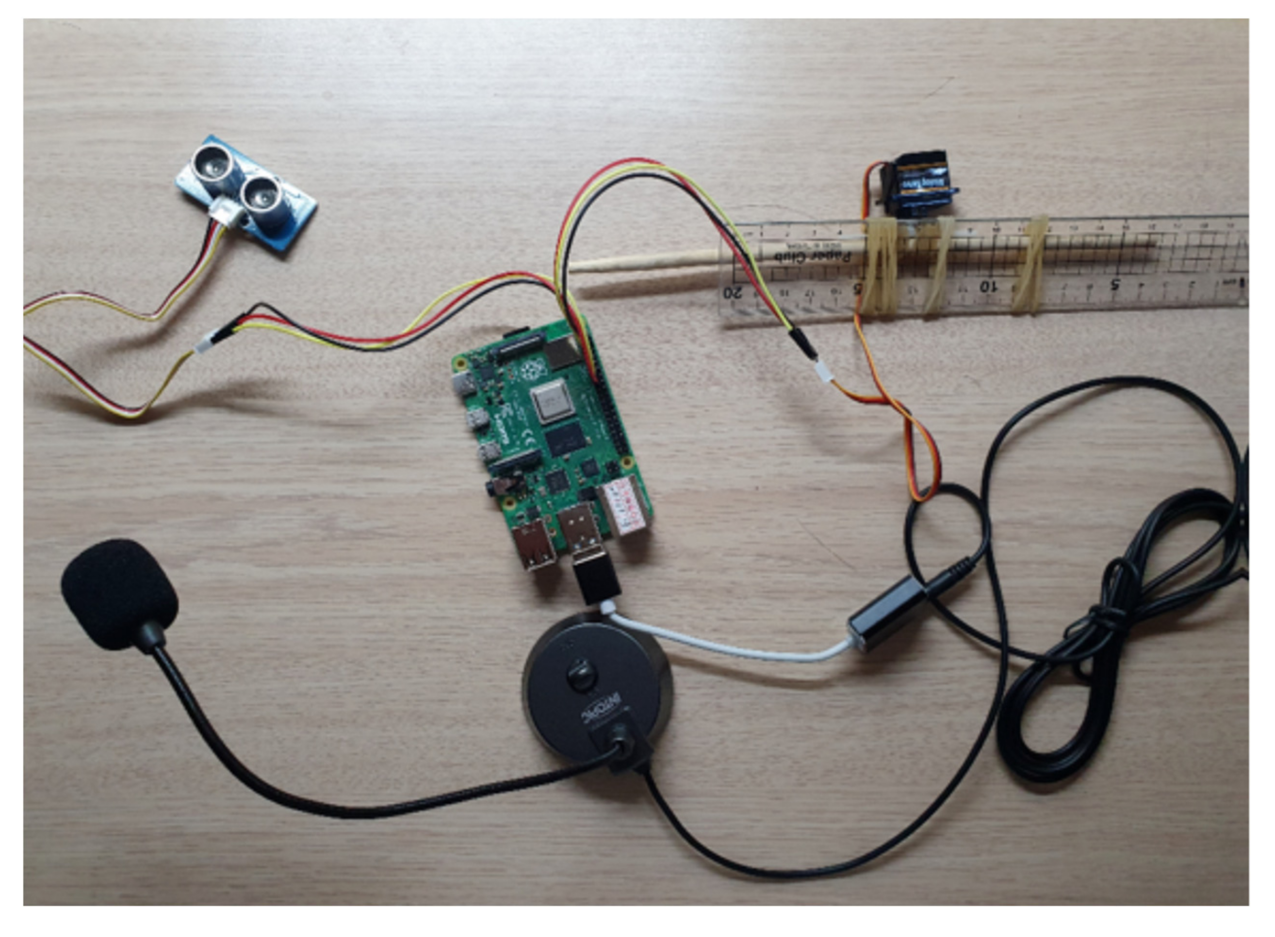
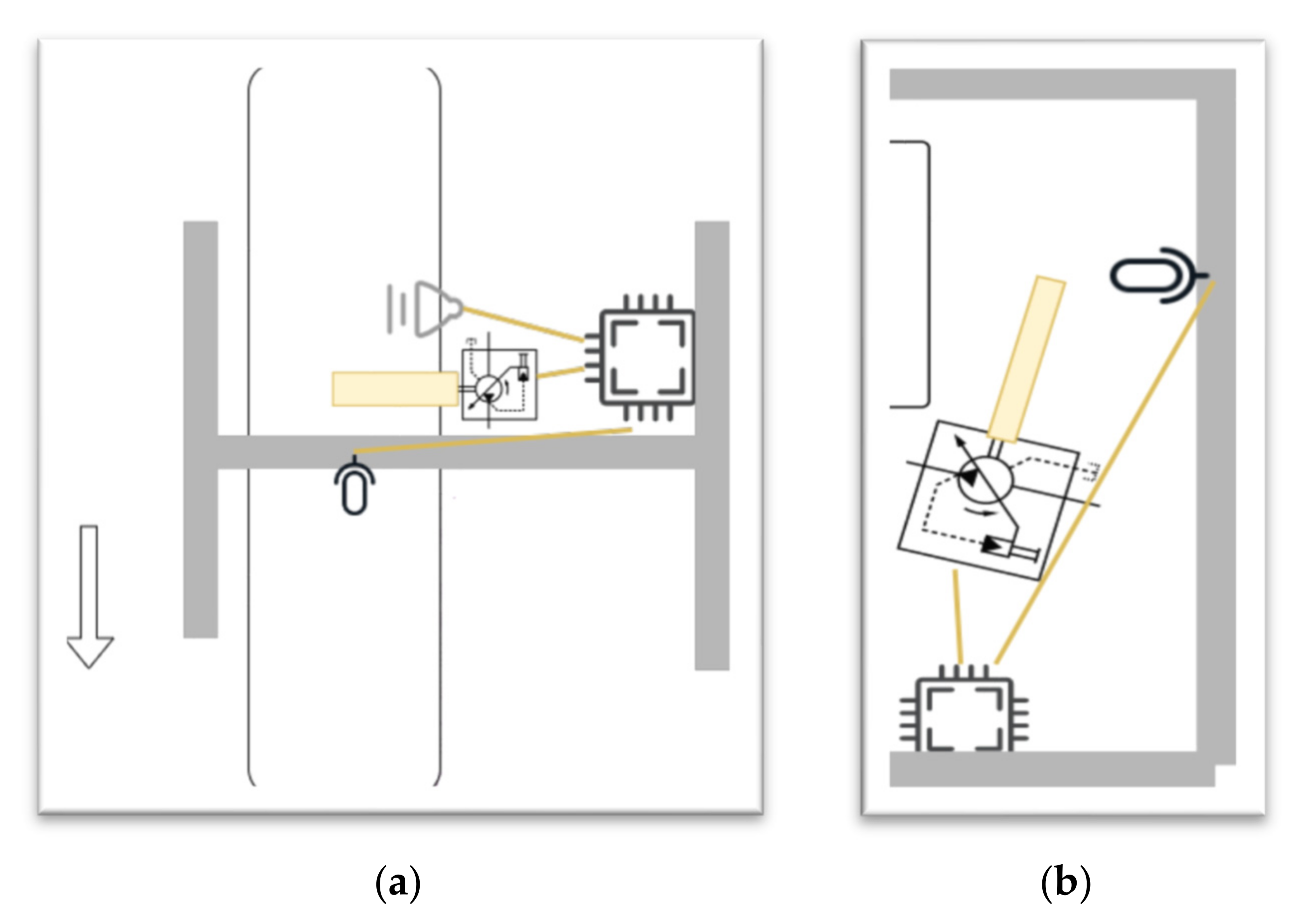
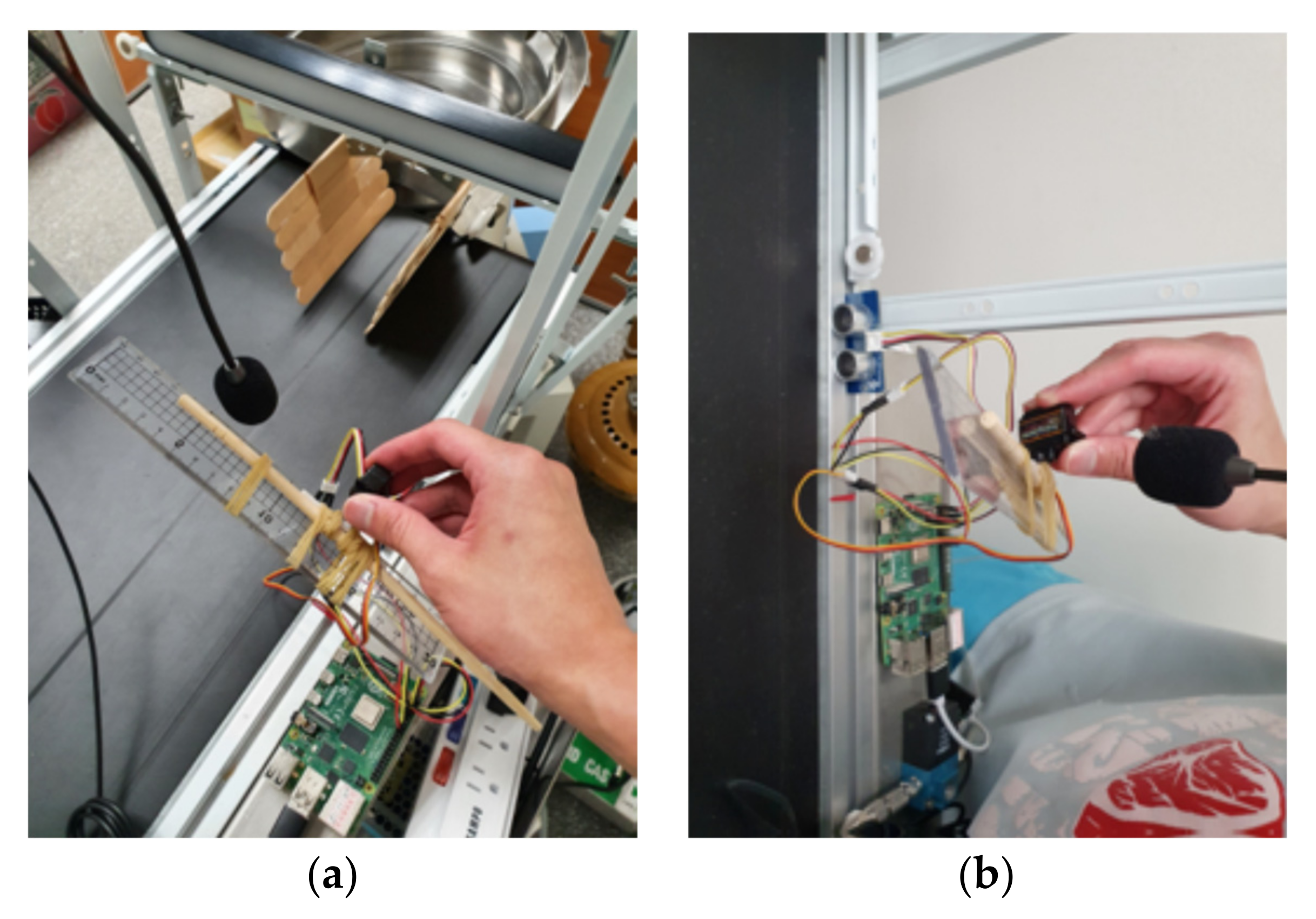
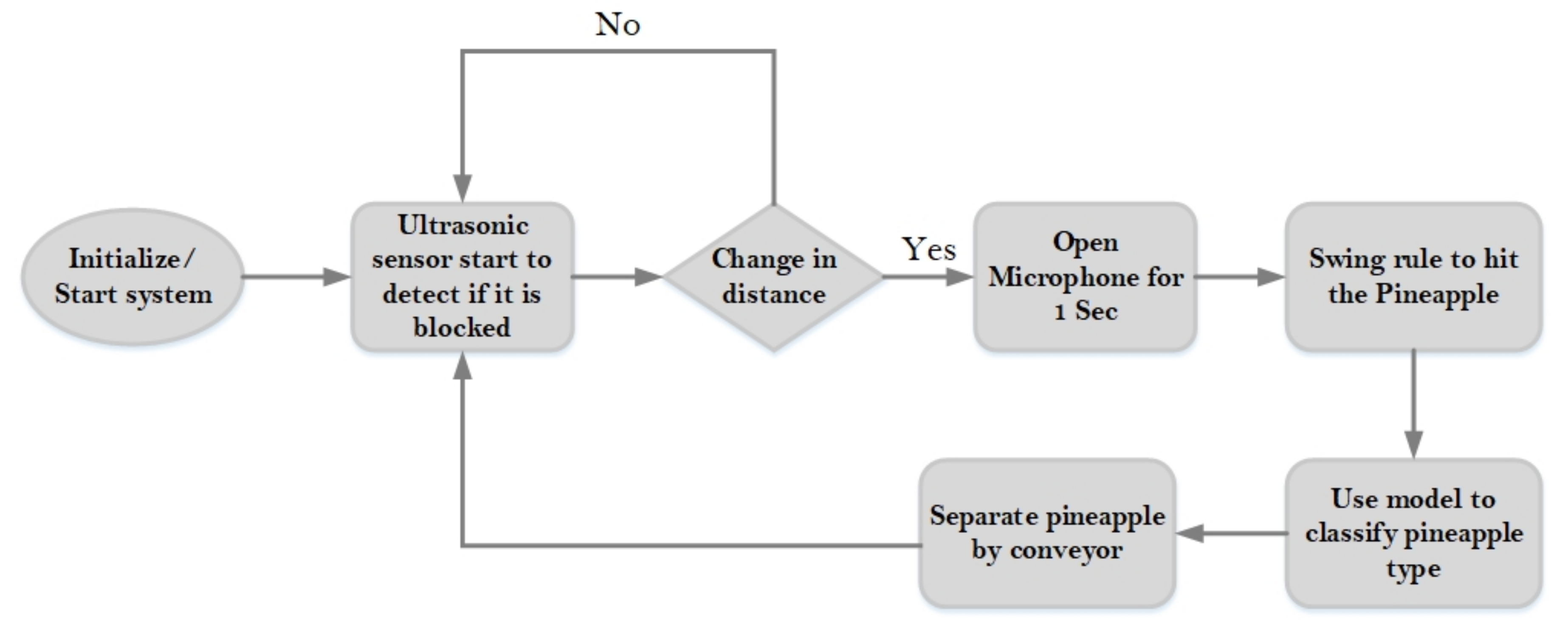
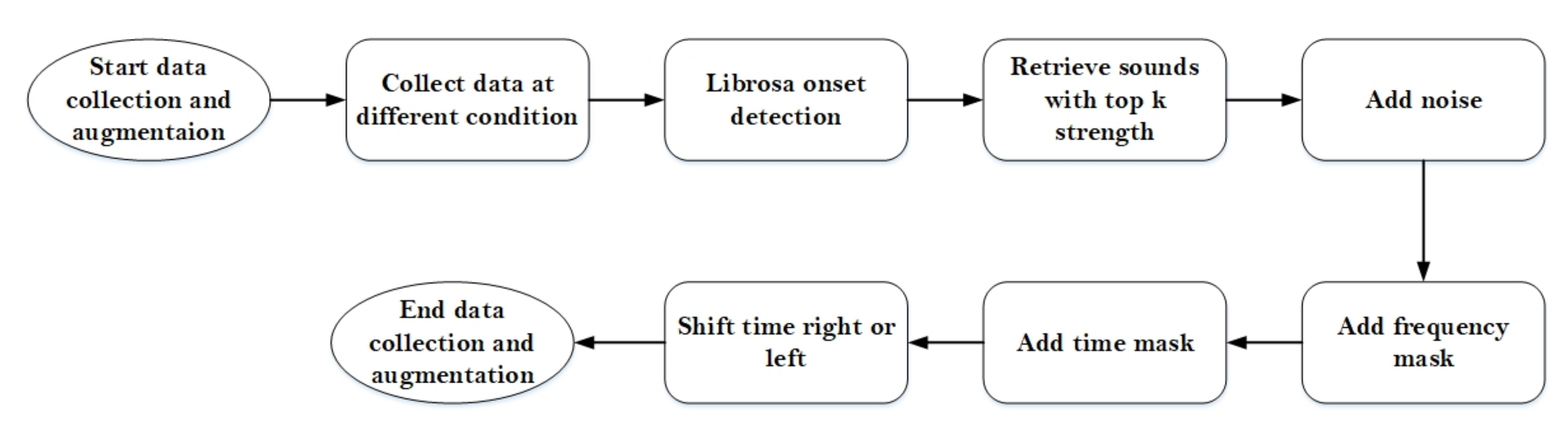
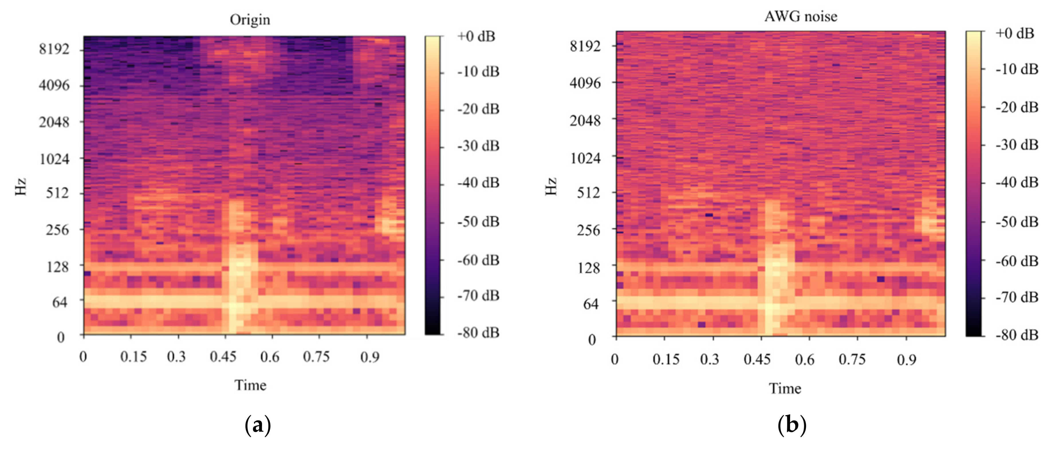
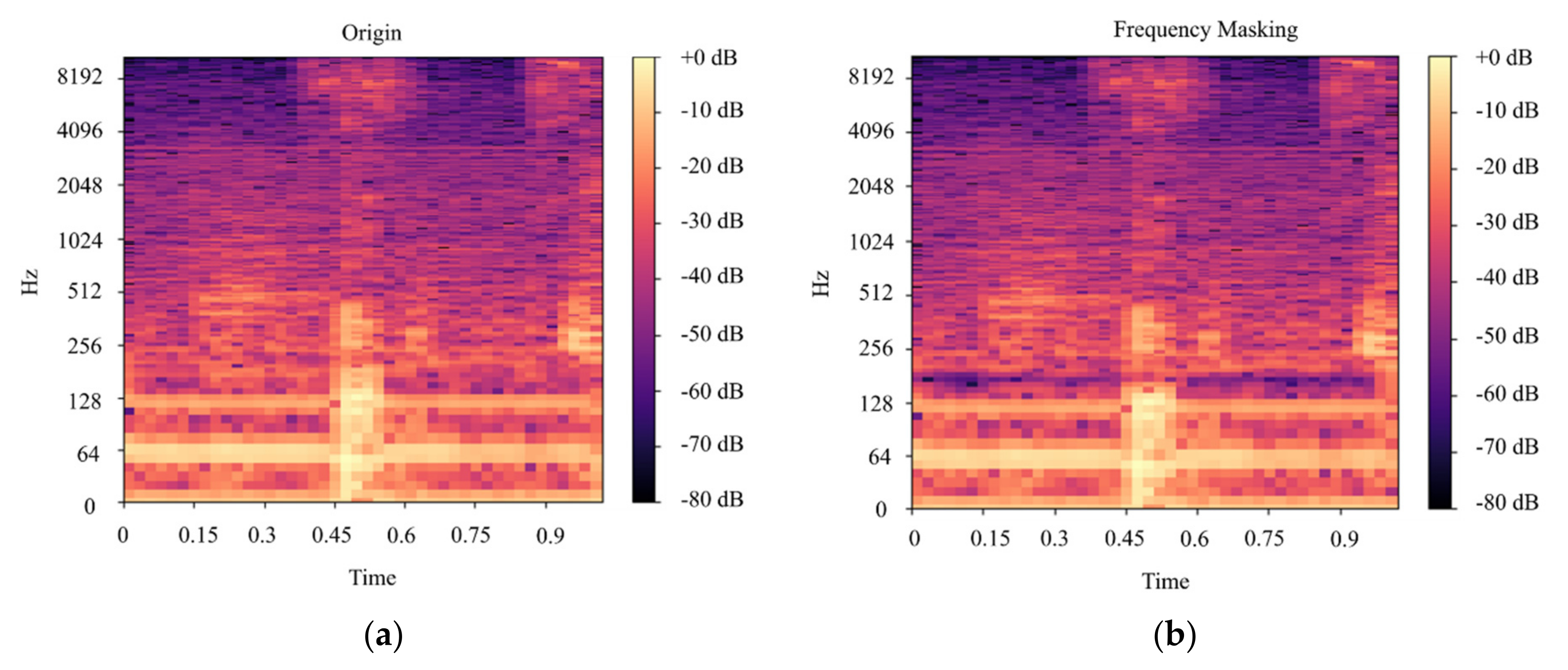
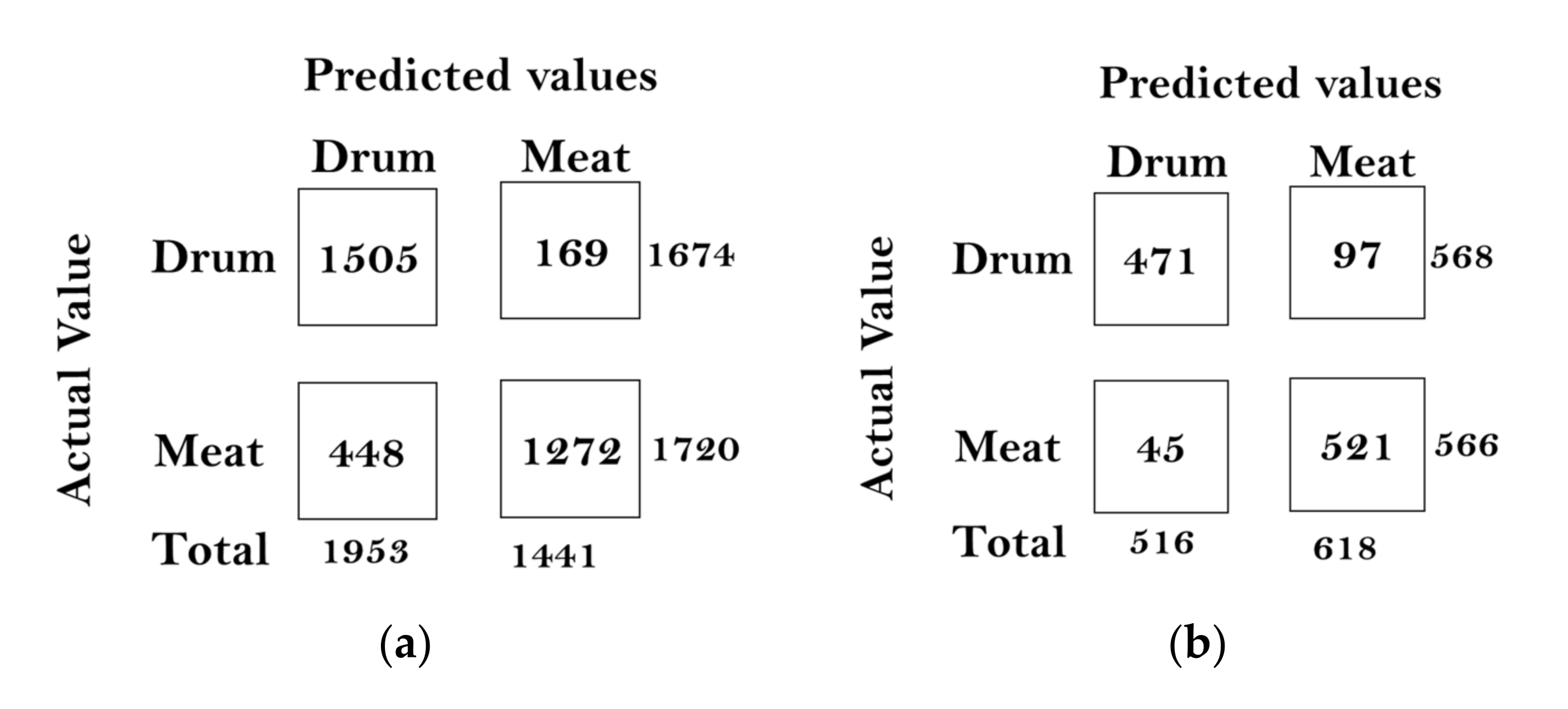
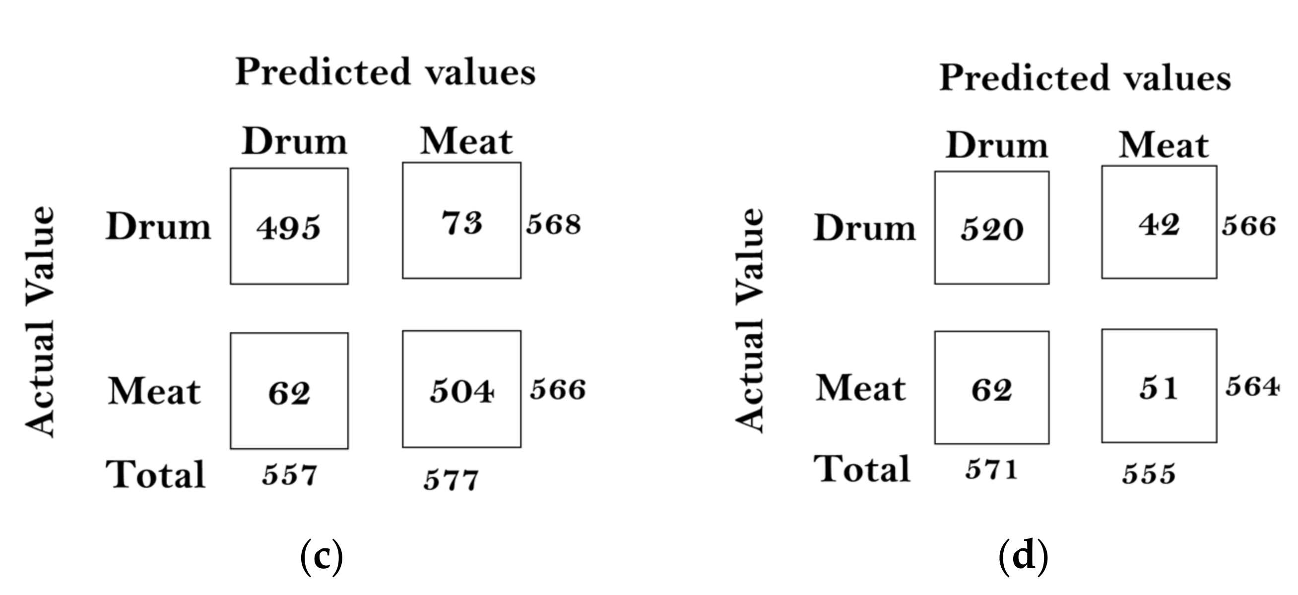
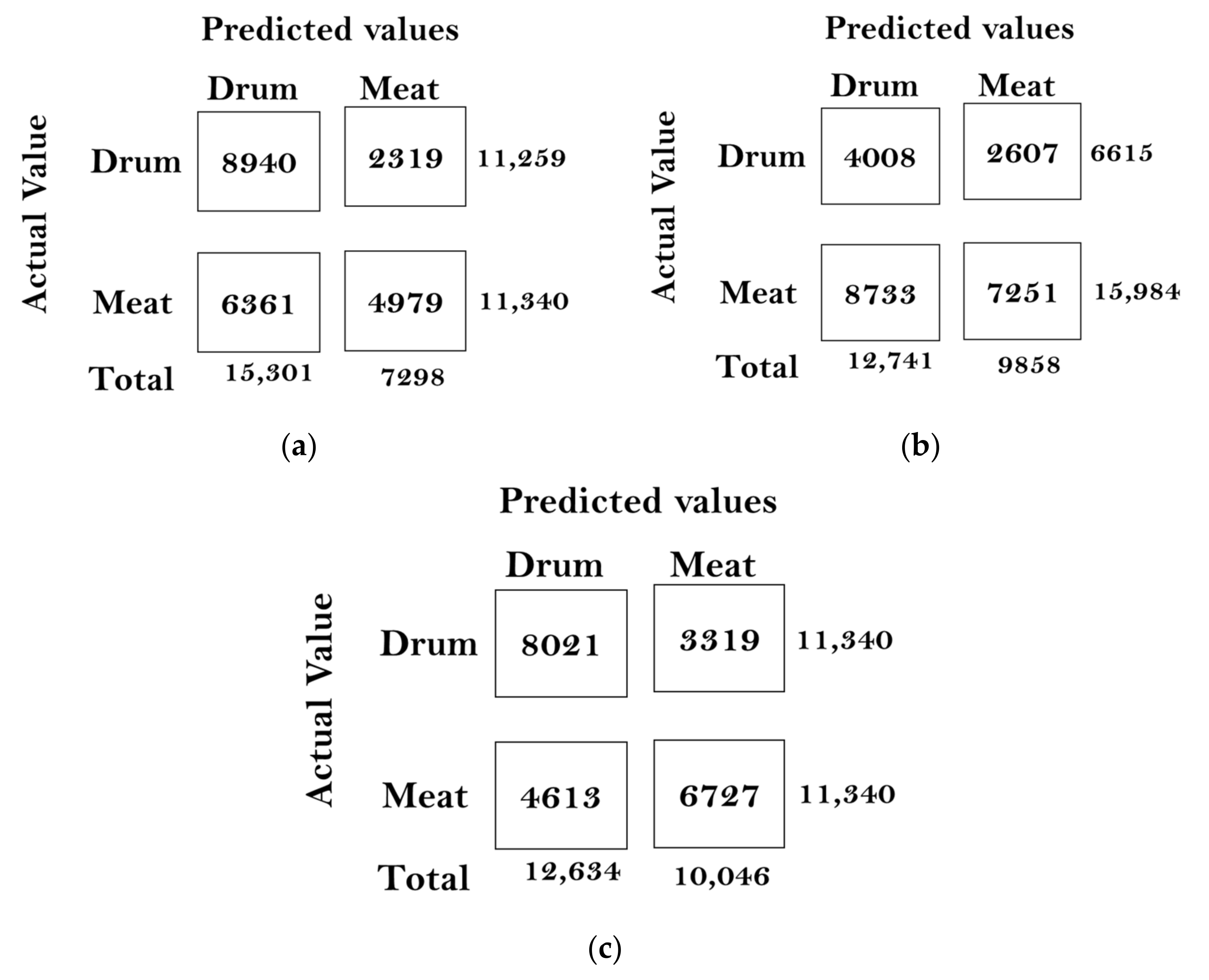
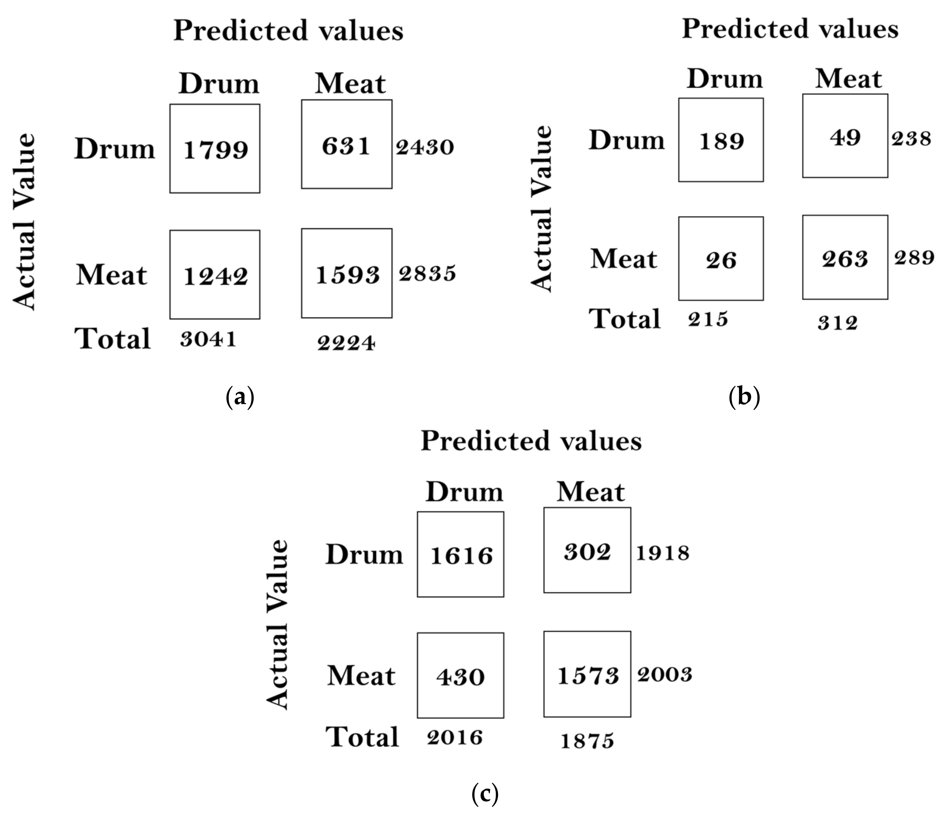
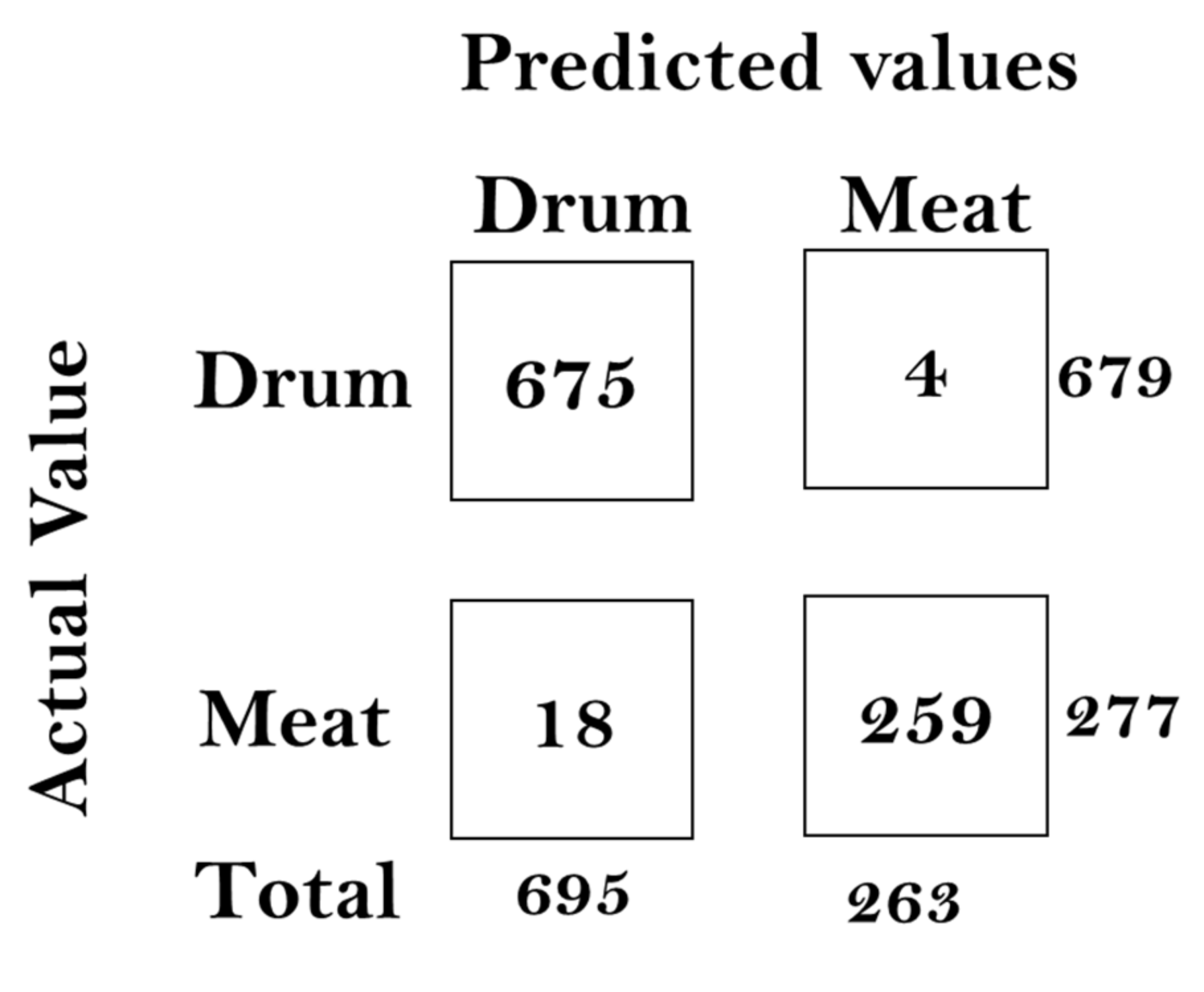
In this paper, we built a model that could classify pineapples, and we built an automatic machine to conduct the whole process. To classify pineapples, we proposed a method related to acoustic spectrograms, which use acoustic data to generate spectrograms. We used our machine to hit pineapples and recorded the hitting sounds to generate spectrograms from the acoustic data. The hitting sounds were transformed from amplitude/time domain to frequency/time domain by the short Fourier transform to create the spectrograms. The spectrograms were used as input to the CNN. Seven different data groups with different conditions and factors were collected from different pineapple batches in farm and factory environments. The highest accuracy of the CNN reached around 0.97 for data Group V when we divided one data group into a training and testing data set; however, when we used the trained from one group and tested the model by another set, the accuracy dropped to 0.54. The accuracy of the developed CNN model is 0.91 for data Group I, 0.88 for data Group II, 0.83 for data group III, 0.87 for data group IV, 0.97 for data Group V, and 0.87 for combined data Groups VI and VII. From the model accuracy and confusion matrices of the developed model, we found that the batches are essential factors for pineapple classification. The sounds of hitting pineapples would change if the data were collected on different days. The developed model reduces the time and cost of the pineapple classification process and increases the accuracy of classification by automating the process of differentiating the drum and meat sound pineapples. Thus, it helps farmers to classify pineapples efficiently. The developed hitting machine, along with the artificial intelligence model, would be significant for farmers around the world, regarding the classification of pineapples

Our current model works on one batch of pineapples and produces less accuracy on another batch. To overcome this, we need to collect more data to make the model more generalized. Our classification machine is still a prototype, which cannot be used as such in farms as it can be damaged easily, so we need to make it more stable. Moreover, according to the latest research by the Taiwan Agriculture Research Institute Council of Agriculture, Executive Yuan [18], the distribution of water might be another reason making the drum sound pineapple and the meat sound pineapple different. We could also train our quantification model with resistance data.

References

1. Chen, C.-Z.; Su, Y.-J.; Lai, Y.-X. Let’s Eat Pineapple in Summer! It’s an Anti-Inflammatory Food and Also Promotes Human Body’s Digestion. Available online: https://health.gvm.com.tw/article/66387 (accessed on 13 October 2021).
2. Statistics Data from Council of Agriculture. Available online: https://www.coa.gov.tw/ws.php?id=2512263 (accessed on 13 October 2021).
3. Buy Directly from Farmers, the Classification Method for Meat Sound Pineapple and Drum Sound Pineapple. Available online: https://www.ishs-horticulture.org/workinggroups/pineapple/PineNews12.pdf (accessed on 13 October 2021).
4. Development and Application of Agricultural Production Automation. Available online: https://www.coa.gov.tw/ws.php?id=9390 (accessed on 13 October 2021).
5. Kharamat, W.; Wongsaisuwan, M.; Wattanamongkhol, N. Durian Ripeness Classification from the Knocking Sounds Using Convolutional Neural Network. In Proceedings of the 2020 8th International Electrical Engineering Congress (iEECON), Chiang Mai, Thailand, 4–6 March 2020. [Google Scholar]
6. Melfrequency Cepstrum. Available online: https://en.wikipedia.org/wiki/Mel-frequency_cepstrum (accessed on 1 November 2021).
7. Baltazar, A.; Aranda, J.I.; González-Aguilar, G. Bayesian classification of ripening stages of tomato fruit using acoustic impact and colorimeter sensor data. Comput. Electron. Agric. 2008, 60, 113–121. [Google Scholar] [CrossRef]
8. Barnea, D.I.; Silverman, H.F. A class of algorithms for fast digital image registration. IEEE Trans. Comput. 1972, 100, 179–186. [Google Scholar] [CrossRef]
9. Feature Scaling. Available online: https://en.wikipedia.org/wiki/Feature_scaling (accessed on 5 November 2021).
10. Berrar, D. Bayes’ theorem and naive Bayes classifier. Encyclopedia of Bioinformatics and Computational Biology: ABC of Bioinformatics; Elsevier Science Publisher: Amsterdam, The Netherlands, 2018; pp. 403–412. [Google Scholar]
11. Mishra, P.; Woltering, E.; Brouwer, B.; van Echtelt, E.H. Improving moisture and soluble solids content prediction in pear fruit using near-infrared spectroscopy with variable selection and model updating approach. Postharvest Biol. Technol. 2021, 171, 111348. [Google Scholar] [CrossRef]
12. Palmer, J.W.; Harker, F.R.; Tustin, D.S.; Johnston, J. Fruit dry matter concentration: A new quality metric for apples. J. Sci. Food Agric. 2010, 90, 2586–2594. [Google Scholar] [CrossRef] [PubMed]
13. Geladi, P.; Kowalski, B.R. Partial least-squares regression: A tutorial. Anal. Chim. Acta 1986, 185, 1–17. [Google Scholar] [CrossRef]
14. Roger, J.; Palagos, B.; Bertrand, D.; Fernandez-Ahumada, E. CovSel: Variable selection for highly multivariate and multi-response calibration: Application to IR spectroscopy. Chemom. Intell. Lab. Syst. 2011, 106, 216–223. [Google Scholar] [CrossRef] [Green Version]
15. Haff, R.; Slaughter, D.C.; Sarig, Y.; Kader, A. X-ray assessment of translucency in pineapple. J. Food Process. Preser. 2006, 30, 527–533. [Google Scholar] [CrossRef] [Green Version]
16. Sperandei, S. Understanding logistic regression analysis. Biochem. Medica 2014, 24, 12–18. [Google Scholar] [CrossRef]
17. Pathaveerat, S.; Terdwongworakul, A.; Phaungsombut, A. Multivariate data analysis for classification of pineapple maturity. J. Food Eng. 2008, 89, 112–118. [Google Scholar] [CrossRef]
18. You, S.-F. High Water Content Is Not the Reason of the Apperance of Meat Sound Pineapple. Resistance Technique from TARI Helps Classification. Available online: https://www.agriharvest.tw/archives/68133 (accessed on 14 August 2021).
19. Resistance Product. Available online: https://www.tari.gov.tw/news/index-1.asp?Parser=9\%2C4\%2C28\%2C\%2C\%2C\%2C4013&fbclid=IwAR0sKpMOBC46p5MyFx6haWqm6GorpvtGyclguqoucP7OHTQTeGie6AxcYw (accessed on 15 November 2021).
20. Gu, J.; Wang, Z.; Kuen, J.; Ma, L.; Shahroudy, A.; Shuai, B.; Liu, T.; Wang, X.; Wang, G.; Cai, J.; et al. Recent advances in convolutional neural networks. Pattern Recogn. 2018, 77, 354–377. [Google Scholar] [CrossRef] [Green Version]
21. McFee, B.; Raffel, C.; Liang, D.; Ellis, D.P.; McVicar, M.; Battenberg, E.; Nieto, O. Librosa: Audio and music signal analysis in python. In Proceedings of the 14th Python in Science Conference, Austin, TX, USA, 6–12 July 2015; pp. 18–24. [Google Scholar]
22. Park, D.S.; Chan, W.; Zhang, Y.; Chiu, C.-C.; Zoph, B.; Cubuk, D.; Le, Q.V. Specaugment: A simple data augmentation method for automatic speech recognition. arXiv 2019, arXiv:1904.08779. [Google Scholar]
23. Ding, L.; Wang, H.-N.; Chetn, J.; Gualn, Z.-H. Tracking under additive white Gaussian noise effect. IET Control Theory Appl. 2010, 4, 2471–2478. [Google Scholar] [CrossRef]
24. Whibley, S.; Day, M.; May, P.; Pennock, M. WAV Format Preservation Assessment; British Library: London, UK, 2016. [Google Scholar]
25. Kay, S. Can detectability be improved by adding noise? IEEE Signal Process. Lett. 2000, 7, 8–10. [Google Scholar] [CrossRef]
26. Skoglund, J.; Kleijn, W.B. On time-frequency masking in voiced speech. IEEE Trans. Speech Audio Process. 2000, 8, 361–369. [Google Scholar] [CrossRef] [Green Version]
27. Wang, D. Time-frequency masking for speech separation and its potential for hearing aid design. Trends Amplif. 2008, 12, 332–353. [Google Scholar] [CrossRef] [PubMed] [Green Version]
28. Zhu, B.; Li, W.; Wang, Z.; Xue, X. A novel audio fingerprinting method robust to time scale modification and pitch shifting. In Proceedings of the 18th ACM International Conference on Multimedia, Yokohama, Japan, 25–29 October 2010; pp. 987–990. [Google Scholar]
29. Tao, R.; Li, Y.-L.; Wang, Y. Short-time fractional Fourier transform and its applications. IEEE Trans. Signal Process. 2009, 58, 2568–2580. [Google Scholar] [CrossRef]
30. Matlab: Shorttime Fourier Transform. Available online: https://www.mathworks.com/help/signal/ref/stft.html (accessed on 25 November 2021).
31. Dieleman, S.; Schrauwen, B. End-to-end learning for music audio. In In Proceedings of the 2014 IEEE International Conference on Acoustics, Speech and Signal Processing (ICASSP), Florence, Italy, 4–9 May 2014. [Google Scholar]
Figure 1. Time and resource-consuming classification of pineapples; (a) transportation, (b) conveyor classification by weight, (c) sound test classification, (d) cleaning, and (e) final classified pineapples.
Agriculture 12 00129 g001
Figure 2. The batting machine.
Agriculture 12 00129 g002
Figure 3. System schematic diagram: (a) top view, (b) side view.
Agriculture 12 00129 g003
Figure 4. System developed in the lab: (a) top view, (b) side view.
Agriculture 12 00129 g004
Figure 5. Flowchart of the proposed automatic classification system.
Agriculture 12 00129 g005
Figure 6. Flowchart of data collection.
Agriculture 12 00129 g006
Figure 7. Spectrograms before and after adding noise operation. (a) Original spectrogram, (b) spectrogram after adding AWG noise.
Agriculture 12 00129 g007
Figure 8. Spectrogram before and after frequency masking operation, (a) Original spectrogram, (b) spectrogram after frequency masking.
Agriculture 12 00129 g008
Figure 9. Spectrogram before and after time masking operation. (a) Original spectrogram, (b) spectrogram after time masking.
Agriculture 12 00129 g009
Figure 10. Spectrogram before and after shifting operation. (a) Original spectrogram, (b) spectrogram after shifting left.
Agriculture 12 00129 g010
Figure 11. Audio signal after STFT. (a) Amplitude/time domain, (b) frequency/time domain.
Agriculture 12 00129 g011
Figure 12. Hit sound spectrogram.
Agriculture 12 00129 g012
Figure 13. The Architecture of the CNN model for acoustic classification.
Agriculture 12 00129 g013
Figure 14. The confusion matrices (a) Group I, (b) Group I upper part, (c) Group I middle part, and (d) bottom part.
Agriculture 12 00129 g014aAgriculture 12 00129 g014b
Figure 15. The confusion matrices (a) training on upper and testing on the middle and bottom parts; (b) training on the middle and testing on the upper and bottom parts; and (c) training on the bottom and testing on the upper and middle parts.
Agriculture 12 00129 g015
Figure 16. The confusion matrices (a) train on Group I and test on Group II, (b) Group II, and (c) combining Groups I and II.
Agriculture 12 00129 g016
Figure 17. The confusion matrix of Group V.
Agriculture 12 00129 g017