
Utility of Deep Learning Algorithms in Initial Flowering Period Prediction Models

Abstract
:1. Introduction
2. Materials and Methods
2.1. Studied Species
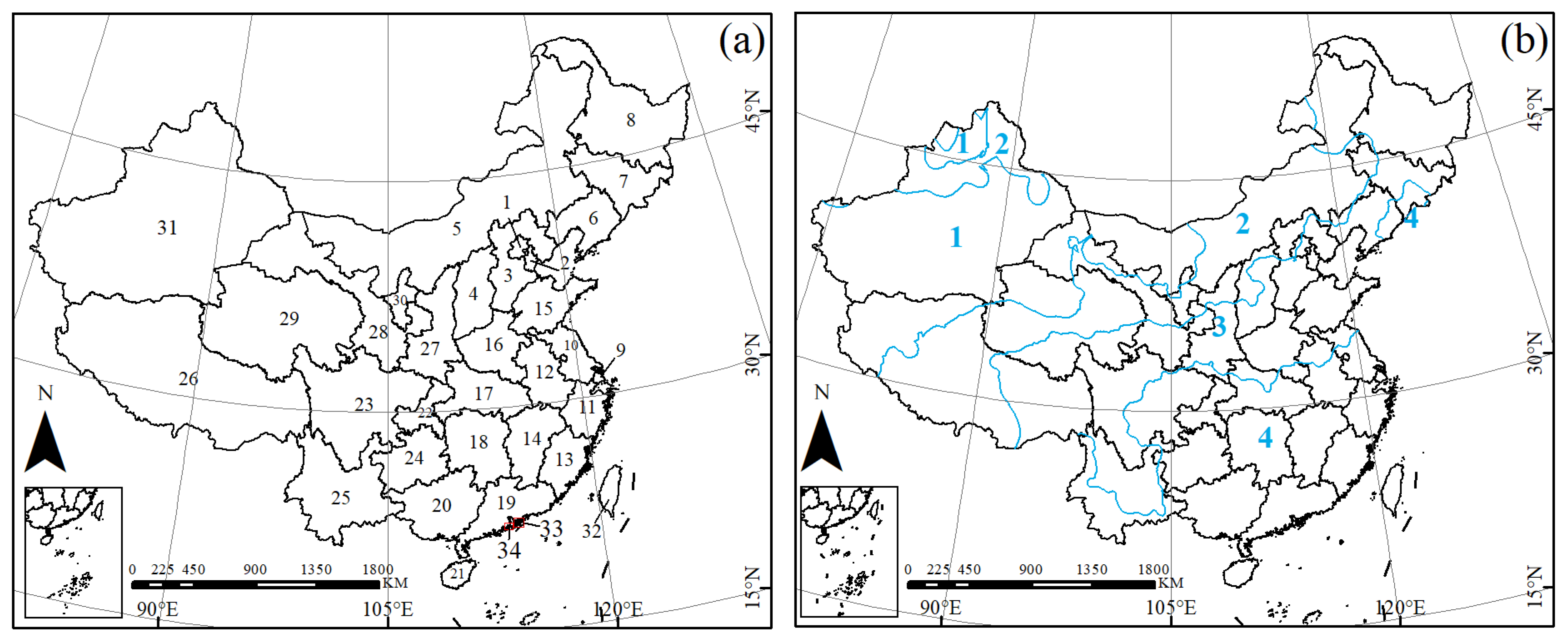
2.2. Region
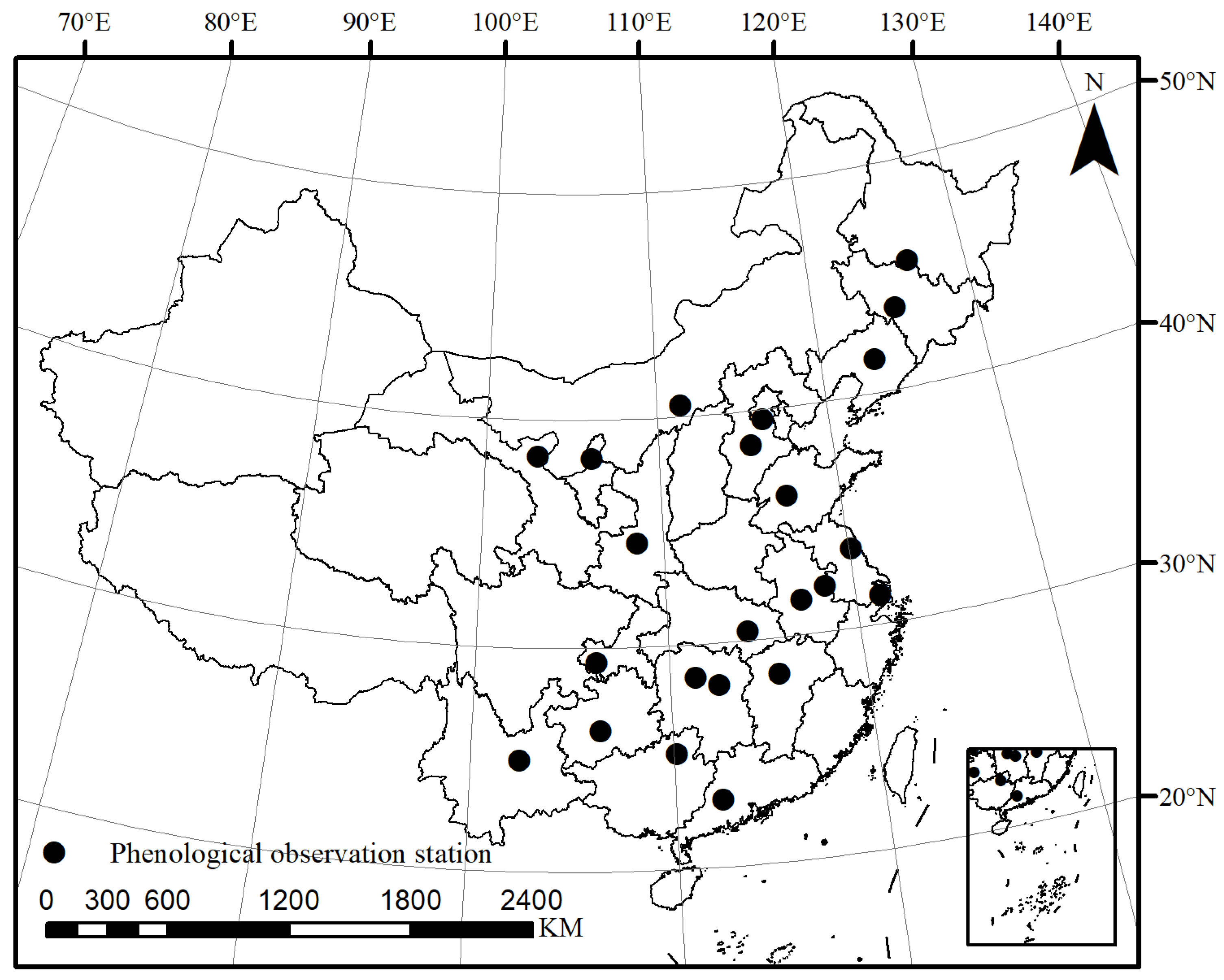
2.3. Materials
2.4. Methods
2.4.1. Selection of Meteorological Factors
2.4.2. Data Processing
2.4.3. Deep Learning Model
- Compared with other neural networks, the RNN can predict the current input value by combining the input values of the first N time series, that is, it has correlation in the time series.
- LSTM can learn the long-term dependence between two variables and retain the error, which can be maintained at a constant level when backpropagation is carried out along the time layer [34,35]. LSTM is equipped with three gating devices to filter the input data, namely, the input gate, forget gate and output gate. The forget gate will generate a value between 0 and 1 according to the output and current input of the previous time to decide whether to retain the information of the previous time [35]. The time function of the forget gate is mainly controlled by the sigmoid activation function:where is the forget gate, is the weight matrix, is the offset term, and is the sigmoid activation function. The closer the value of is to 0, the more items will be forgotten.
- Compared with the LSTM model, the GRU simplifies the calculation steps and substantially increases the training speed, while the GRU also uses a gate device to filter information, namely, the reset gate and update gate. In the process of training, the input information will not be cleared by the gate device, but the necessary information will be retained in the next cycle, and the information will be saved to avoid the problem of gradient disappearance. Since there are only two gate structures, the actual running time of the GRU model is substantially less than that of LSTM with fewer network parameters, so the risk of GRU model overfitting is smaller under the condition of ensuring accuracy.
2.4.4. Training Effect Indicators
2.4.5. Interpretability Model Based on SHAP
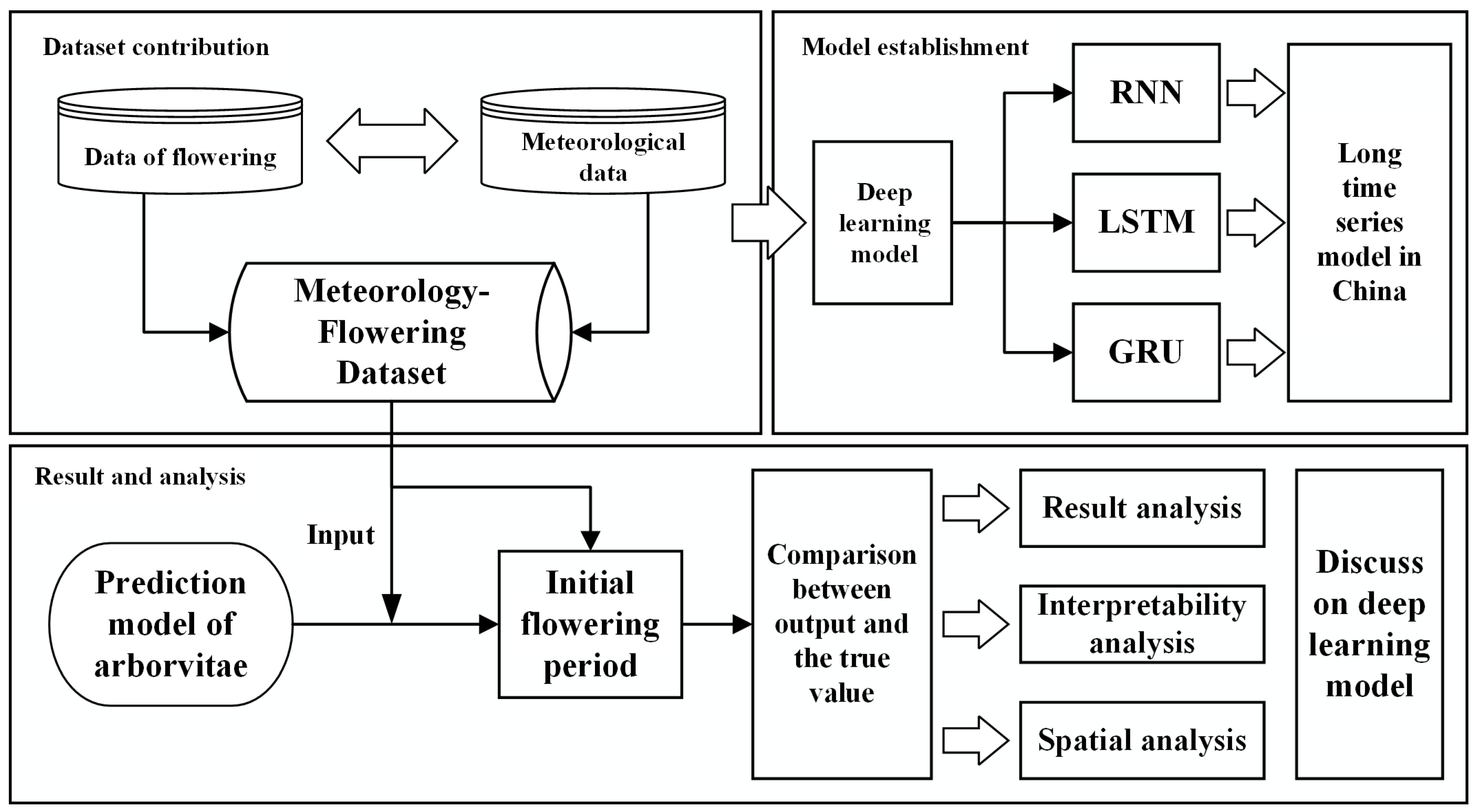
2.4.6. Overall Process of Predicting the Initial Flowering Period in DL
3. Results
3.1. Basic Characteristics of P. orientalis during Initial Flowering
3.2. Model Training Effect
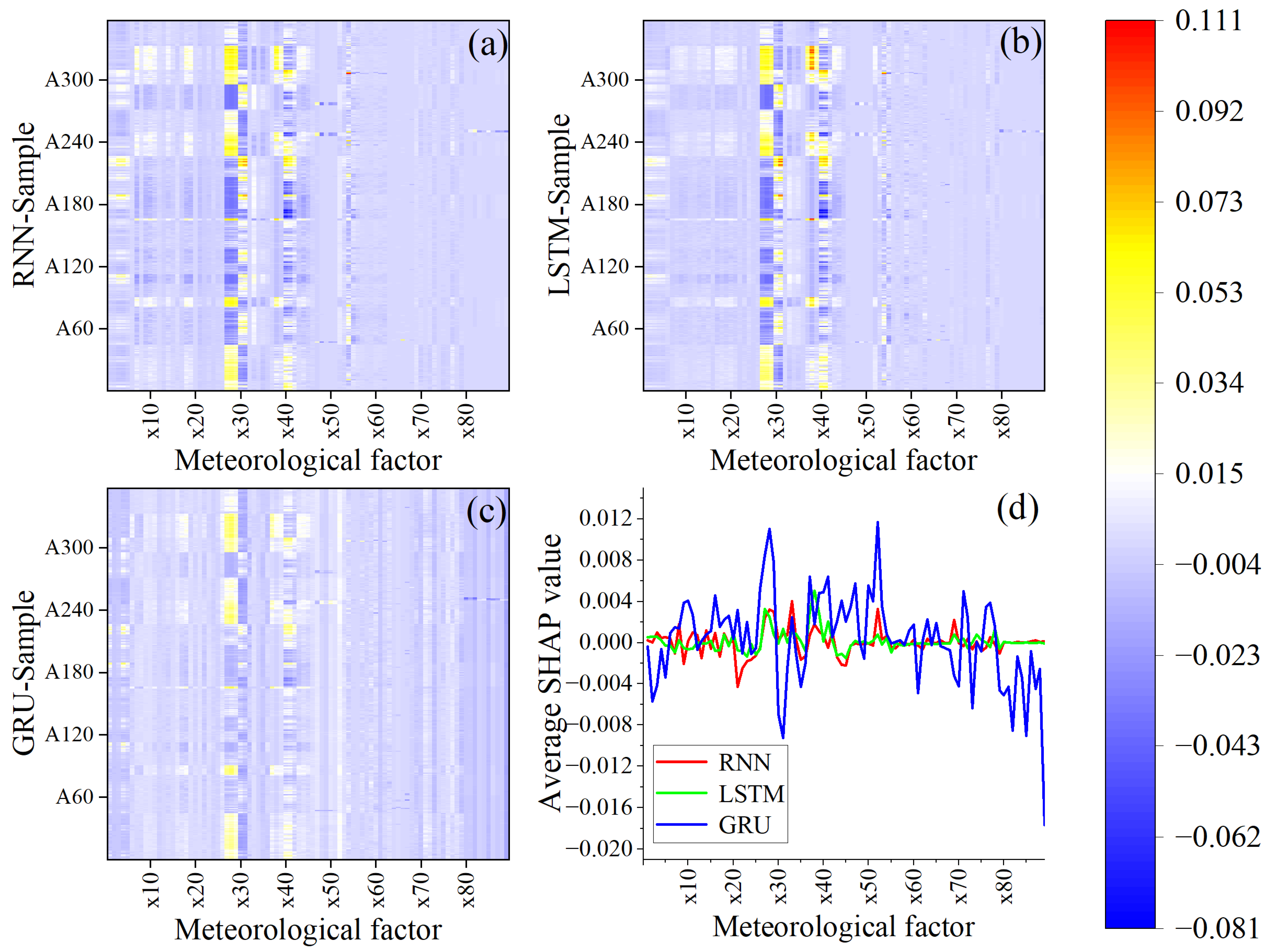
3.3. Interpretability of DL Models
3.4. Comparison between DL and the Traditional Prediction Model
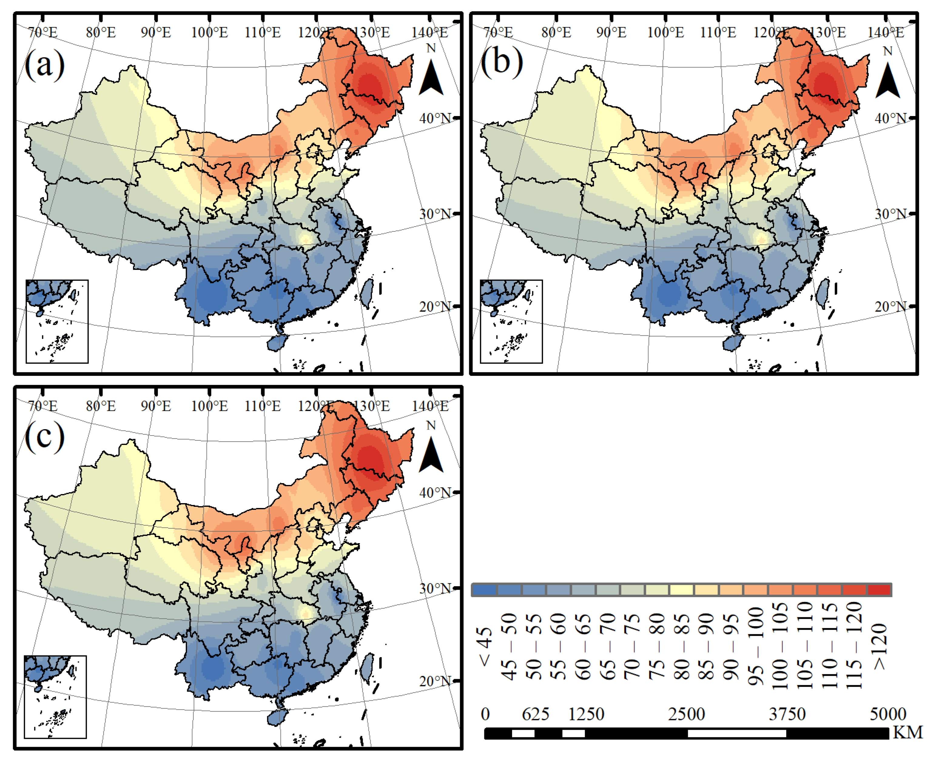
3.5. Spatial Distribution and Interpolation of Prediction for DL
4. Discussion
5. Conclusions
- (1)
- The initial flowering in China mainly occurs from the beginning of February to the end of April, and it has spatial differences, which are later in northern China than in southern China.
- (2)
- The DL model is suitable for nationwide flowering prediction in China, and the average error of DL is only within 2 d.
- (3)
- Comparing the RNN, LSTM and the GRU, we find that the GRU is more suitable for the prediction model of initial flowering, with higher accuracy and more stable spatial predictions.
- (4)
- The initial flowering period of P. orientalis in China presents obvious hierarchical characteristics, which are mainly manifested in the southern region where the flowering period is the earliest. With the increase in latitude, the initial flowering period gradually increases from south to north.
Author Contributions
Funding
Institutional Review Board Statement
Informed Consent Statement
Data Availability Statement
Acknowledgments
Conflicts of Interest
References
- Root, T.L.; Price, J.T.; Hall, K.R.; Schneider, S.H.; Rosenzweig, C.; Pounds, J.A. Fingerprints of Global Warming on Wild Animals and Plants. Nature 2003, 421, 57–60. [Google Scholar] [CrossRef] [PubMed]
- Walther, G.-R.; Post, E.; Convey, P.; Menzel, A.; Parmesan, C.; Beebee, T.J.C.; Fromentin, J.-M.; Hoegh-Guldberg, O.; Bairlein, F. Ecological Responses to Recent Climate Change. Nature 2002, 416, 389–395. [Google Scholar] [CrossRef] [PubMed]
- Cleland, E.; Chuine, I.; Menzel, A.; Mooney, H.; Schwartz, M. Shifting Plant Phenology in Response to Global Change. Trends Ecol. Evol. 2007, 22, 357–365. [Google Scholar] [CrossRef] [PubMed]
- Parmesan, C.; Yohe, G. A Globally Coherent Fingerprint of Climate Change Impacts across Natural Systems. Nature 2003, 421, 37–42. [Google Scholar] [CrossRef]
- Bandoc, G.; Piticar, A.; Patriche, C.; Roșca, B.; Dragomir, E. Climate Warming-Induced Changes in Plant Phenology in the Most Important Agricultural Region of Romania. Sustainability 2022, 14, 2776. [Google Scholar] [CrossRef]
- García-Mozo, H.; López-Orozco, R.; Oteros, J.; Galán, C. Factors Driving Autumn Quercus Flowering in a Thermo-Mediterranean Area. Agronomy 2022, 12, 2596. [Google Scholar] [CrossRef]
- Linderholm, H.W. Growing Season Changes in the Last Century. Agric. For. Meteorol. 2006, 137, 1–14. [Google Scholar] [CrossRef]
- Sparks, T. Local-Scale Adaptation to Climate Change: The Village Flower Festival. Clim. Res. 2014, 60, 87–89. [Google Scholar] [CrossRef] [Green Version]
- Wang, L.; Ning, Z.; Wang, H.; Ge, Q. Impact of Climate Variability on Flowering Phenology and Its Implications for the Schedule of Blossom Festivals. Sustainability 2017, 9, 1127. [Google Scholar] [CrossRef] [Green Version]
- Tao, Z.; Ge, Q.; Wang, H.; Dai, J. Phenological Basis of Determining Tourism Seasons for Ornamental Plants in Central and Eastern China. J. Geogr. Sci. 2015, 25, 1343–1356. [Google Scholar] [CrossRef]
- Wolkovich, E.M.; Cook, B.I.; Allen, J.M.; Crimmins, T.M.; Betancourt, J.L.; Travers, S.E.; Pau, S.; Regetz, J.; Davies, T.J.; Kraft, N.J.B.; et al. Warming Experiments Underpredict Plant Phenological Responses to Climate Change. Nature 2012, 485, 494–497. [Google Scholar] [CrossRef] [PubMed]
- Chmielewski, F.-M.; Rötzer, T. Response of Tree Phenology to Climate Change across Europe. Agric. For. Meteorol. 2001, 108, 101–112. [Google Scholar] [CrossRef]
- Linkosalo, T.; Hakkinen, R.; Hanninen, H. Models of the Spring Phenology of Boreal and Temperate Trees: Is There Something Missing? Tree Physiol. 2006, 26, 1165–1172. [Google Scholar] [CrossRef] [PubMed]
- Moussus, J.-P.; Julliard, R.; Jiguet, F. Featuring 10 Phenological Estimators Using Simulated Data: Featuring the Behaviour of Phenological Estimators. Methods Ecol. Evol. 2010, 1, 140–150. [Google Scholar] [CrossRef]
- Verbesselt, J.; Hyndman, R.; Zeileis, A.; Culvenor, D. Phenological Change Detection While Accounting for Abrupt and Gradual Trends in Satellite Image Time Series. Remote Sens. Environ. 2010, 114, 2970–2980. [Google Scholar] [CrossRef] [Green Version]
- Arlo Richardson, E.; Seeley, S.D.; Walker, D.R. A Model for Estimating the Completion of Rest for ‘Redhaven’ and ‘Elberta’ Peach Trees. Hortscience 1974, 9, 331–332. [Google Scholar] [CrossRef]
- White, L.M. Relationship between Meteorological Measurements and Flowering of Index Species to Flowering of 53 Plant Species. Agric. Meteorol. 1979, 20, 189–204. [Google Scholar] [CrossRef]
- Anderson, J.L.; Richardson, E.A.; Kesner, C.D. Validation of Chill Unit and Flower Bud Phenology Models for “Montmorency” Sour Cherry. Acta Hortic. 1986, 184, 71–78. [Google Scholar] [CrossRef]
- Hakkinen, R.; Linkosalo, T.; Hari, P. Effects of Dormancy and Environmental Factors on Timing of Bud Burst in Betula Pendula. Tree Physiol. 1998, 18, 707–712. [Google Scholar] [CrossRef] [Green Version]
- Demeloabreu, J. Modelling Olive Flowering Date Using Chilling for Dormancy Release and Thermal Time. Agric. For. Meteorol. 2004, 125, 117–127. [Google Scholar] [CrossRef]
- Chauhan, Y.S.; Ryan, M.; Chandra, S.; Sadras, V.O. Accounting for Soil Moisture Improves Prediction of Flowering Time in Chickpea and Wheat. Sci. Rep. 2019, 9, 7510. [Google Scholar] [CrossRef] [PubMed] [Green Version]
- Wu, D.; Huo, Z.; Wang, P.; Wang, J.; Jiang, H.; Bai, Q.; Yang, J. The Applicability of Mechanism Phenology Models to Simulating Apple Flowering Date in Shaanxi Province. J. Appl. Meteor. Sci. 2019, 30, 555–564. [Google Scholar] [CrossRef]
- Tan, J.; Chen, Z.; Xiao, M. Characteristics and forecast of flowering duration of Cherry Blossoms in Wuhan University. Acta Ecol. Sin. 2021, 41, 38–47. [Google Scholar] [CrossRef]
- Puchałka, R.; Klisz, M.; Koniakin, S.; Czortek, P.; Dylewski, Ł.; Paź-Dyderska, S.; Vítková, M.; Sádlo, J.; Rašomavičius, V.; Čarni, A.; et al. Citizen Science Helps Predictions of Climate Change Impact on Flowering Phenology: A Study on Anemone Nemorosa. Agric. For. Meteorol. 2022, 325, 109133. [Google Scholar] [CrossRef]
- Wang, L.; Zhou, X.; Zhu, X.; Dong, Z.; Guo, W. Estimation of Biomass in Wheat Using Random Forest Regression Algorithm and Remote Sensing Data. Crop J. 2016, 4, 212–219. [Google Scholar] [CrossRef] [Green Version]
- Jiang, P.; Shi, J.; Niu, P.X.; Yue, L.U. Effects on Activities of Defensive Enzymes and MDA Content in Leaves of Platycladus Orientalis under Naturally Decreasing Temperature. J. Shihezi Univ. (Nat. Sci.) 2009, 127, 487–493. [Google Scholar] [CrossRef]
- Li, X.P.; He, Y.P.; Wu, X.J.; Ren, Q.F. Water Stress Experiments of Platycladus Orientalis and Pinns Tablaeformis Young Trees. For. Res. 2011, 24, 91–96. [Google Scholar] [CrossRef]
- Wang, F.; Wu, D.; Haruhiko, Y.; Xing, S.; Zang, L. Digital Image Analysis of Different Crown Shape of Platycladus Orientalis. Ecol. Inform. 2016, 34, 146–152. [Google Scholar] [CrossRef]
- An Editorial Committee of Flora of China. Flora of China; Science Press: Beijing, China; Missouri Botanical Garden Press: St. Louis, MO, USA, 1999; Volume 4. [Google Scholar]
- Yearbook of the People’s Republic of China Climate. Available online: http://www.gov.cn/guoqing/2005-09/13/content_2582628.htm (accessed on 3 December 2022).
- Xu, J.; Wang, D.; Qiu, X.; Zeng, Y.; Zhu, X.; Li, M.; He, Y.; Shi, G. Dominant Factor of Dry-wet Change in China since 1960s. Int. J. Climatol. 2021, 41, 1039–1055. [Google Scholar] [CrossRef]
- Mi, Q.; Gao, X.; Li, Y.; Li, X.; Tang, Y.; Ren, C. Application of Deep Learning Method to Drought Prediction. J. Appl. Meteorol. Sci. 2022, 33, 104–114. [Google Scholar]
- Deo, R.C.; Şahin, M. Application of the Artificial Neural Network Model for Prediction of Monthly Standardized Precipitation and Evapotranspiration Index Using Hydrometeorological Parameters and Climate Indices in Eastern Australia. Atmos. Res. 2015, 161–162, 65–81. [Google Scholar] [CrossRef]
- Hochreiter, S.; Schmidhuber, J. Long Short-Term Memory. Neural Comput. 1997, 9, 1735–1780. [Google Scholar] [CrossRef] [PubMed]
- Gers, F.A. Learning to Forget: Continual Prediction with LSTM. Neural Comput. 2000, 12, 2451–2471. [Google Scholar] [CrossRef] [PubMed]
- Amin, M.; Akram, M.N.; Ramzan, Q. Bayesian Estimation of Ridge Parameter under Different Loss Functions. Commun. Stat. Theory Methods 2022, 51, 4055–4071. [Google Scholar] [CrossRef]
- Lundberg, S.; Lee, S.-I. A Unified Approach to Interpreting Model Predictions. Adv. Neural Inf. Process. Syst. 2017, 30, 1–10. [Google Scholar]
- Inouye, D.W. Effects of Climate Change on Phenology, Frost Damage, and Floral Abundance of Montane Wildflowers. Ecology 2008, 89, 353–362. [Google Scholar] [CrossRef] [PubMed] [Green Version]
- Park, I.W.; Mazer, S.J. Overlooked Climate Parameters Best Predict Flowering Onset: Assessing Phenological Models Using the Elastic Net. Glob. Chang. Biol. 2018, 24, 5972–5984. [Google Scholar] [CrossRef]
- Chen, Z.; Xiao, M.; Chen, X. Change in Flowering Dates of Japanese Cherry Blossoms (P. Yedoensis Mats.) in Wuhan University Campus and Its Relationship with Variability of Winter Temperature. Acta Ecol. Sin. 2008, 28, 5209–5217. [Google Scholar]
- Menzel, A.; Sparks, T.H.; Estrella, N.; Koch, E.; Aasa, A.; Ahas, R.; Alm-Kübler, K.; Bissolli, P.; Braslavská, O.; Briede, A.; et al. European Phenological Response to Climate Change Matches the Warming Pattern: European Phenological Response to Climate Change. Glob. Chang. Biol. 2006, 12, 1969–1976. [Google Scholar] [CrossRef]
- Abu-Asab, M.S.; Peterson, P.M.; Shetler, S.G.; Orli, S.S. Earlier Plant Flowering in Spring as a Response to Global Warming in the Washington, DC, Area. Biodivers. Conserv. 2001, 10, 597–612. [Google Scholar] [CrossRef]
- Zhou, L. Relation between Interannual Variations in Satellite Measures of Northern Forest Greenness and Climate between 1982 and 1999. J. Geophys. Res. 2003, 108, 4004. [Google Scholar] [CrossRef] [Green Version]
- Fitter, A.H.; Fitter, R.S.R.; Harris, I.T.B.; Williamson, M.H. Relationships Between First Flowering Date and Temperature in the Flora of a Locality in Central England. Funct. Ecol. 1995, 9, 55. [Google Scholar] [CrossRef]
- Krüger, E.; Woznicki, T.L.; Heide, O.M.; Kusnierek, K.; Rivero, R.; Masny, A.; Sowik, I.; Brauksiepe, B.; Eimert, K.; Mott, D.; et al. Flowering Phenology of Six Seasonal-Flowering Strawberry Cultivars in a Coordinated European Study. Horticulturae 2022, 8, 933. [Google Scholar] [CrossRef]
- Bonelli, M.; Eustacchio, E.; Avesani, D.; Michelsen, V.; Falaschi, M.; Caccianiga, M.; Gobbi, M.; Casartelli, M. The Early Season Community of Flower-Visiting Arthropods in a High-Altitude Alpine Environment. Insects 2022, 13, 393. [Google Scholar] [CrossRef]
- Monder, M.J. Trends in the Phenology of Climber Roses under Changing Climate Conditions in the Mazovia Lowland in Central Europe. Appl. Sci. 2022, 12, 4259. [Google Scholar] [CrossRef]
- Tooke, F.; Battey, N.H. Temperate Flowering Phenology. J. Exp. Bot. 2010, 61, 2853–2862. [Google Scholar] [CrossRef] [Green Version]
- Shi, Y.; Shen, Y.; Kang, E.; Li, D.; Ding, Y.; Zhang, G.; Hu, R. Recent and Future Climate Change in Northwest China. Clim. Chang. 2007, 80, 379–393. [Google Scholar] [CrossRef]
- Shi, P.; Sun, S.; Wang, M.; Li, N.; Wang, J.; Jin, Y.; Gu, X.; Yin, W. Climate Change Regionalization in China (1961–2010). Sci. China Earth Sci. 2014, 57, 2676–2689. [Google Scholar] [CrossRef]


| Meteorological Elements | Meteorological Factors | Number of Factors |
|---|---|---|
| Temperature |
| 46 |
| Ground temperature |
| 7 |
| Precipitation |
| 10 |
| Hours of sunshine |
| 5 |
| Relative humidity |
| 11 |
| Pressure |
| 10 |
| Station | Average Value (d) | Minimum Value (d) | Maximum Value (d) | Range (d) | Standard Deviation (d) | Skewness | Kurtosis |
|---|---|---|---|---|---|---|---|
| Baoding | 95.00 | 76 | 111 | 35 | 10.29 | −0.16 | −0.28 |
| Beijing | 86.97 | 65 | 108 | 43 | 10.03 | 0.12 | −0.59 |
| Changde | 59.88 | 38 | 78 | 40 | 10.06 | −0.27 | 0.026 |
| Guiyang | 57.05 | 33 | 86 | 53 | 13.89 | −0.11 | −0.44 |
| Hohhot | 108.00 | 101 | 121 | 20 | 6.31 | 0.97 | 0.19 |
| Shanghai | 63.38 | 50 | 76 | 26 | 7.61 | −0.04 | −0.07 |
| Foshan | 48.78 | 32 | 65 | 33 | 12.27 | −0.08 | −1.88 |
| Nanjing | 44.90 | 31 | 55 | 24 | 7.30 | −0.36 | −0.69 |
| Nanchang | 55.78 | 25 | 76 | 51 | 13.43 | −0.58 | 0.34 |
| Hefei | 63.93 | 41 | 78 | 37 | 11.11 | −0.67 | −0.70 |
| Harbin | 130.50 | 129 | 132 | 3 | 1.50 | 0.01 | 0.01 |
| Kunming | 40.08 | 5 | 98 | 93 | 23.96 | 0.93 | 0.95 |
| Guilin | 43.35 | 22 | 74 | 52 | 16.51 | 0.80 | −0.33 |
| Wuhan | 88.05 | 52 | 112 | 60 | 18.94 | −0.41 | −1.17 |
| Minqin | 104.93 | 92 | 136 | 44 | 10.76 | 1.61 | 4.07 |
| Shenyang | 111.20 | 104 | 122 | 18 | 7.33 | 0.69 | −2.49 |
| Tai’an | 76.25 | 70 | 86 | 16 | 6.01 | 1.29 | 1.78 |
| Xi’an | 65.86 | 46 | 81 | 35 | 8.20 | −0.43 | 0.51 |
| Chongqing | 54.62 | 24 | 76 | 52 | 14.99 | −0.39 | −1.05 |
| Yinchuan | 110.21 | 84 | 123 | 39 | 12.90 | −0.83 | −0.67 |
| Changchun | 111.96 | 93 | 129 | 36 | 7.91 | 0.12 | 0.89 |
| Changsha | 54.00 | 45 | 63 | 18 | 9.00 | 0.01 | 0.01 |
| Yancheng | 68.09 | 44 | 80 | 36 | 8.09 | −1.09 | 1.69 |
| Models and Indicators | RNN | LSTM | GRU |
|---|---|---|---|
| MAE | 1.50 × 10⁻² | 5.18 × 10⁻⁴ | 2.16 × 10⁻⁴ |
| MAPE | 4.56 | 0.16 | 0.05 |
| R2 | 0.99 | 0.99 | 0.99 |
| Model | Deep Learning Model | Multiple Linear Regression Model | ||||
|---|---|---|---|---|---|---|
| Indicator | RNN | LSTM | GRU | Mean | ||
| MAE | 1.50 × 10⁻² | 5.18 × 10⁻⁴ | 2.16 × 10⁻⁴ | 5.12 × 10⁻³ | 0.06 | |
| MAPE | 4.56 | 0.16 | 0.053 | 1.59 | 15.45 | |
| R2 | 0.99 | 0.99 | 0.99 | 0.99 | 0.84 | |
Publisher’s Note: MDPI stays neutral with regard to jurisdictional claims in published maps and institutional affiliations. |
© 2022 by the authors. Licensee MDPI, Basel, Switzerland. This article is an open access article distributed under the terms and conditions of the Creative Commons Attribution (CC BY) license (https://creativecommons.org/licenses/by/4.0/).
Share and Cite
Jiao, G.; Shentu, X.; Zhu, X.; Song, W.; Song, Y.; Yang, K. Utility of Deep Learning Algorithms in Initial Flowering Period Prediction Models. Agriculture 2022, 12, 2161. https://doi.org/10.3390/agriculture12122161
Jiao G, Shentu X, Zhu X, Song W, Song Y, Yang K. Utility of Deep Learning Algorithms in Initial Flowering Period Prediction Models. Agriculture. 2022; 12(12):2161. https://doi.org/10.3390/agriculture12122161
Chicago/Turabian StyleJiao, Guanjie, Xiawei Shentu, Xiaochen Zhu, Wenbo Song, Yujia Song, and Kexuan Yang. 2022. "Utility of Deep Learning Algorithms in Initial Flowering Period Prediction Models" Agriculture 12, no. 12: 2161. https://doi.org/10.3390/agriculture12122161