Stability Study of Time Lag Disturbance in an Automatic Tractor Steering System Based on Sliding Mode Predictive Control

Abstract

To improve the working accuracy and anti-interference capability of the steering operation of an automatic tractor, this paper investigates the tractor steering system. In response to the current problems of high steering resistance during tractor field operations and the low service life of the drive shaft of conventional electric steering wheel solutions, an electro-hydraulic coupled power-assisted solution combining EPS and HPS is proposed. The combination of the EPS system’s high control accuracy and sensitive steering operation and the hydraulic power system’s large steering torque greatly reduces the power of the power motor and battery performance requirements, optimizing the power transmission scheme to achieve green and energy-saving purposes. Secondly, the research is focused on the influence of external disturbances on the stability of the steering system during tractor operation, and a combination of model predictive control and sliding mode control is used to study the steering system control strategy. It is finally demonstrated through simulations and experiments that it can compensate for the disturbance of the system control parameters by external disturbances, has the ability of MPC to handle input constraints and maintains the advantages of SMC robustness.

1. Introduction

With the development of industrial modernization, agriculture is also gradually moving towards mechanization and intelligence. In agricultural production, a self-driving tractor can effectively reduce the intensity of operations, and has received a lot of attention by researchers. The automatic steering system is among the most important aspects and has become a hotspot for research. Many control methods have emerged, such as proportional integral differential (PID) control, feedback linearization control, backstepping control, adaptive control, sliding mode control (SMC) and model predictive control (MPC).

Abroshan et al. proposed a fuzzy PID steering control algorithm to improve the response speed and accuracy of the steering system [1]. Liu, J.Y. et al. used a proportional reversing valve to modify the tractor steering, established a multi-loop automatic hydraulic steering system, and designed a PID-based steering control strategy to achieve accurate control of the steering [2]. A backstepping control technique has been used by Huynh et al. (2012) [3] and Fang (2004) [4]. However, the performance of the backstepping controller is more sensitive to the unmatched disturbances. Hence, Javad T. [5] proposed a non-linear disturbance control method based on SMC for tire skidding of tractors. The SMC method is an important robust control method that can effectively handle model uncertainty. Some researchers have used MPC for steer-by-wire systems to solve the problem of large steering tracking errors [6,7]. Borreli et al. [8] proposed an MPC-based active steering controller to solve the constrained optimization problem, which can track the desired path well while ensuring lateral driving stability. Wang et al. [9] used an integral LTV-MPC control strategy to solve the problem of mutual interference between the steering and braking systems in a hierarchical controller, thus ensuring the effectiveness of the tracked path. Huang [10] proposed a robust weighted gain-scheduling H∞ controller for the disturbance caused by the time lag between the power transmission of the steering system. The proposed method is validated by CarSim simulation to reduce the effects of steering lags and time-varying parameters on the steering system. While MPC has unique advantages in dealing with system constraints, some researchers have also gradually used MPC and SMC in combination to address system disturbances and stability requirements. Zhao et al. [11] proposed a passive controller for discrete-time uncertain generalized systems based on SMPC technology to improve the control performance of control systems under time lags.

In the field of vehicle steering systems, hydraulic power steering (HPS) and electric power steering (EPS) are commonly used. The hydraulic power steering not only maintains the clear road feeling compared to mechanical steering, but can also adjust the flow to change the power-assisting characteristics of the steering system [12,13]. However, the energy losses inherent in HPS have limited its development in the direction of electrification. EPS provides the necessary auxiliary power to the steering system through the use of a power-assisted motor, which overcomes the disadvantages of hydraulic power transmission by means of gears, has the advantage of high transmission efficiency, is easy to use and economical, and is widely used in small cars [14]. However, compared with HPS, the road feel of the transmission is poor, while the control accuracy and smoothness is low. Since the output torque of the motor is related to the winding of the coil, the high power motor means that the power supply requirements are high for the large size of the booster motor, and the small space in the cab location results in the installation of motors that do not meet the steering assistance needs of large vehicles. In addition, due to factors such as the safety limitation of circuit board power and the installation space of high-power motors, the assist power provided by the EPS is too small to meet the steering system demand of the vehicles with a large load on the front axle, such as trucks, buses, agricultural and engineering vehicles. Therefore, a number of researchers have investigated the combination of the two power steering systems. Zhao et al. [15] built a test rig to model and validate an electro-hydraulic compound steering (EHCS) system to improve the operational efficiency of bus steering systems and achieve energy savings. The results show that the EHCS system can maintain good road feel and low steering energy consumption.

In practice, the tractor is a non-linear system and there are various disturbances in the environment, so this paper combines sliding mode control (SMC) and model predictive control (MPC) to study the control of an automatic tractor steering system. The use of SMPC can effectively handle the input constraints of MPC and has the robust stability of SMC. An electro-hydraulic coupled steering technique is used for the steering system to build an experimental rig and to establish a relevant control model based on SMPC. Simulations and experiments show that SMPC maintains good robustness and tracking performance in the presence of model uncertainties and disturbances.

The relevant parts of this paper are organized as follows. The electro-hydraulic coupling power steering(EHCPS) system model is developed in Section 2.1. The SMC controller design is discussed in Section 2.2. In Section 2.3, the proposed SMPC is described. The performance of the SMPC controller is demonstrated in Section 2.6. Finally, some conclusions are drawn in Section 4 and the directions for future work are discussed.

2. Materials and Methods

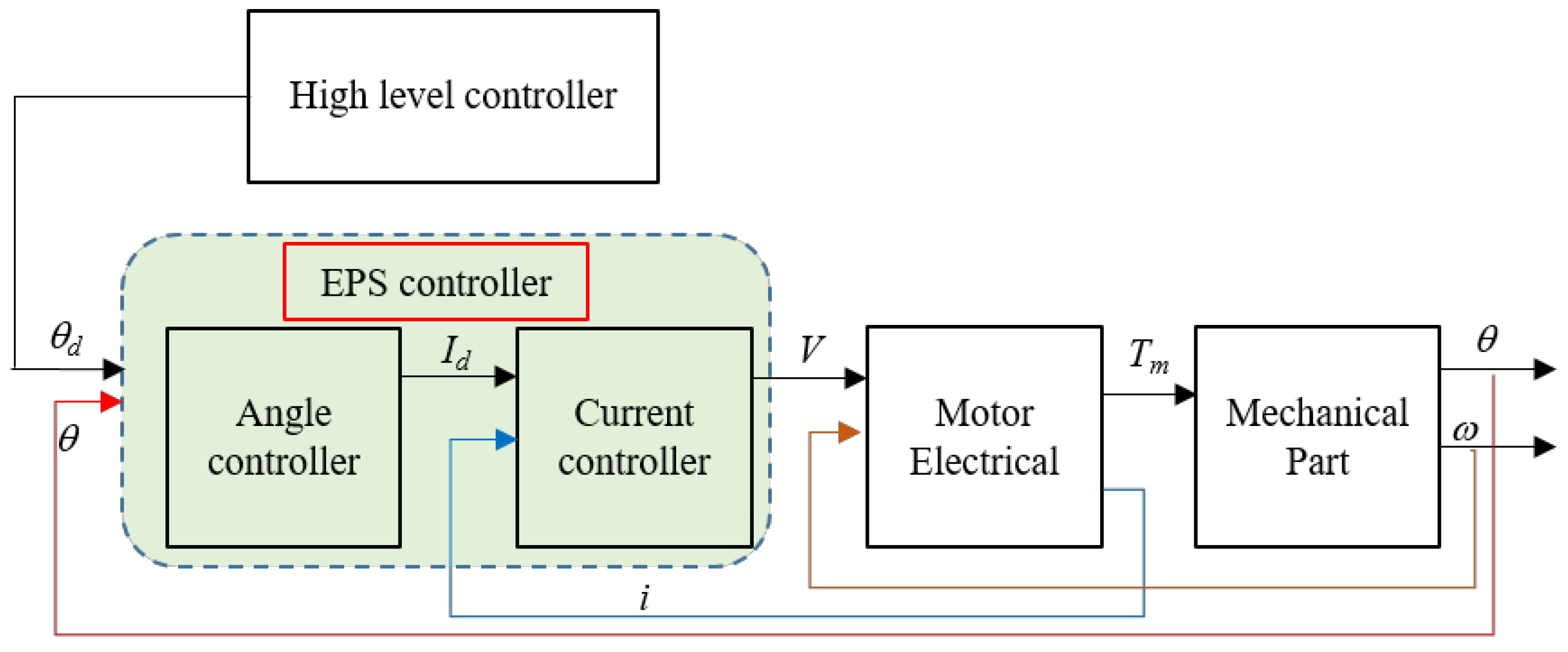
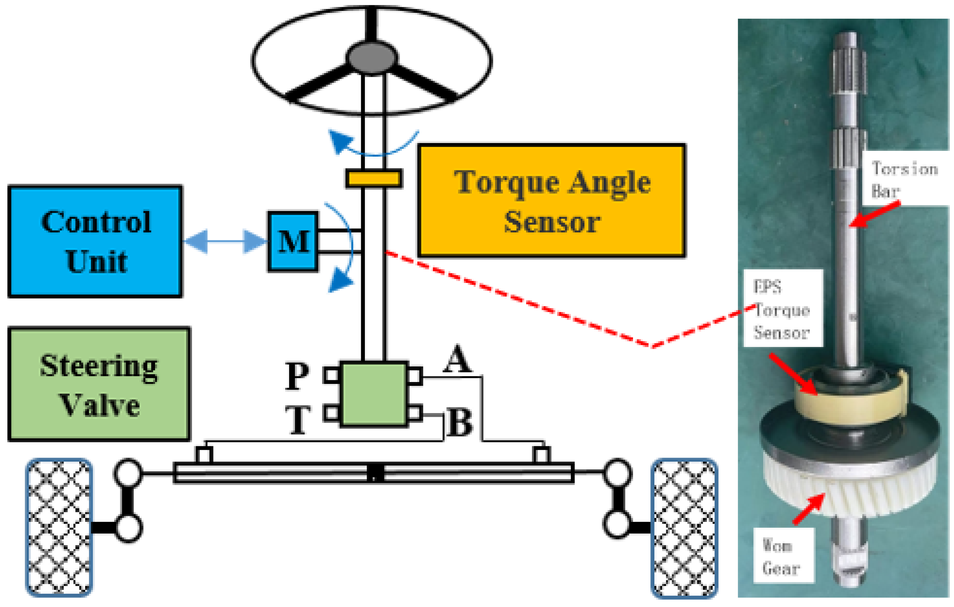
2.1. EHCPS System Modeling

For a self-driving tractor to be operated unmanned, it needs to have the functions of sensing, decision making, control and execution of these components to be performed automatically. In a self-driving tractor, the steering system is used to execute the desired steering angle θ_d output by the high-level control system, and the desired steering angle is tracked by adjusting the motor current I_d output by the EPS controller. As shown in Figure 1.

Controller Modeling

The structure of the electro-hydraulic coupling power steering system (EHCPS) is shown in Figure 2. The system works as follows: Firstly, the controller of the EPS receives the steering wheel rotation angle signal θ_d, and then controls the steering torque T_M output from the motor M, which is applied to the steering column, opening the steering valve through the rotation of the column. The hydraulic fluid flows from port P to the hydraulic cylinder through ports A and B, causing the cylinder to move from side to side and ultimately driving the front wheel.

The total steering resistance moment to be overcome when the front wheels are turned from side to side is given by Taborek’s formula [16]

$$T_{steer}=0.05\times G_f\times \frac{1}{1+e/L_b}\times \frac{L_b}{200}\times \frac{{\mu }_{road}}{0.7}$$

(1)

where $T_{steer}$ is the torque of steer of the road wheel, $G_f$ is the force on steering front axle, e is the King pin off-set (100 mm), and L_b is the tire breadth (165 mm). ${\mu }_{\mathrm{road}}$ is the coefficient of friction between the road surface and the tire, in relation to the operating surface, usually ranges from 0.1 to 0.9, with the coefficient of friction between the tire and the ground in field environments at 0.7.

Maximum working force of the steering cylinder

$$F_{s\max }=T_{steer}/{\mathrm{r}}_{\min }$$

(2)

where r_min is the minimum steering resistance arm.

Operating thrust and working volume of the steering cylinder (balanced cylinder) for the front axle

$$\begin{array}{l}F=P\times \frac{\pi }{4}\times (D^2-{\mathrm{d}}^2)\times 10\\ V=\frac{\pi }{4}\times (D^2-{\mathrm{d}}^2)\times L_{ps}\end{array}$$

(3)

where F is the steering force (N); P is the steering pressure (Pa); D is the internal diameter of cylinder (cm); d is the piston rod diameter (cm); L_ps is the piston stroke (cm); V is the cylinder working volume (cm³).

The operating principle of an EPS based on field-oriented control (FOC) of a permanent magnet synchronous motor (PMSM) is shown in Figure 3.

In the case of a permanent magnet synchronous motor, the equation for the balance of the rotating torque can be expressed as

$$J_R\frac{d^2{\theta }_r}{d^{2}t}+D\frac{d{\theta }_r}{dt}+K{\theta }_r=T_M-T_L$$

(4)

where J_R represents the rotor inertia, θ_r represents the rotor rotation angle, D represents the wind resistance and friction torque coefficient proportional to speed, K represents the torsional elastic torque coefficient, T_M represents the motor torque and T_L represents the load torque.

So the tractor electro-hydraulic coupled steering power system model (EHCPS) was constructed based on the EPS model and torque balance established by Wonhee Kim to model the automatic steering system [17,18].

$$J{\ddot{\delta }}_f{\left(\mathrm{t}\right)+b}_w{\dot{\delta }}_f{\left(\mathrm{t}\right)+k}_c\mathrm{sgn}({\dot{\delta }}_f\left(\mathrm{t}\right))+T_t^f\left(\mathrm{t}\right)=i{T}_M+F{\mathrm{r}}_{\min }$$

(5)

where J and b_w denote the moment of inertia (kg m²) and damping coefficient of the front wheel, respectively; k_c denotes the Coulomb friction constant; δ_f denotes the steering angle; $T_t^f$ denotes the self-aligning torque; i indicates the steering ratio of the booster motor; T_M indicates the motor turning torque; F indicates the operating thrust of the balanced cylinder of the front axle; r_min is the minimum steering resistance arm of the front wheel; $\mathrm{sgn}({\dot{\delta }}_f\left(\mathrm{t}\right))$ is the sign function defined as follows:

$$\begin{array}{l}\mathrm{sgn}({\dot{\delta }}_{sw}\left(\mathrm{t}\right))=\left\{\begin{array}{c}-1,({\dot{\delta }}_f<0)\\ 0,({\dot{\delta }}_f=0)\\ 1,({\dot{\delta }}_f>0)\end{array}\right.\\ T_t^f=-(l_p+l_m)C_f(\beta +\frac{l_f\times \omega }{v_x}-{\delta }_f)\end{array}$$

(6)

In the above equations, $l_p$ and $l_m$ is the pneumatic trail (the distance between the resultant point of application of lateral force and the center of the tire, 0.028 m) and the mechanical trail (distance between the tire center point and the ground point where the tire turns due to the wheel roll angle, 0.05 m), respectively. C_f denotes the front tire cornering stiffness coefficient, $\beta$ denotes the lateral deflection angle, $l_f$ denotes the distance of the front axle to CG (1 m), $\omega$ denotes the yaw rate, $v_x$ denotes the longitudinal component of the center of gravity velocity, and ${\delta }_f$ denotes the steering angle of the front axle.

The output torque $T_M$ of the power steering motor and the thrust F of the hydraulic steering cylinder can be seen as proportional to the input voltage u of the motor

$$\left\{\begin{array}{c}{T}_M=k_{M}u\\ F=k_{BC}u\end{array}\right.$$

(7)

Write EHCPS in the form of a state space equation

$$\left\{\begin{array}{c}\dot{x}=Ax+Bu+B_{T}T\\ y=Cx+Du\end{array}\right.$$

(8)

where the state vector $x$ is $x={\left[\begin{array}{cc}{\dot{\delta }}_f& {\delta }_f\end{array}\right]}^T$; the input vector u is the motor input voltage.

$$\begin{gathered} \left\{\begin{array}{c}\left[\begin{array}{c}{\ddot{\delta }}_f\\ {\dot{\delta }}_f\end{array}\right]=\left[\begin{array}{cc}-\frac{b_w}{J}& 0\\ 1& 0\end{array}\right]\left[\begin{array}{c}{\dot{\delta }}_f\\ {\delta }_f\end{array}\right]+\left[\begin{array}{c}\frac{i{k}_M+k_{BC}{r}_{\min }}{J}\\ 0\end{array}\right]u+\left[\begin{array}{c}\frac{-1}{J}\\ 0\end{array}\begin{array}{c}\frac{-1}{J}\\ 0\end{array}\right]\left[\begin{array}{c}{k}_c\mathrm{sgn}({\dot{\delta }}_f)\\ T_t^f\end{array}\right]\\ y=\left[\begin{array}{cc}0& 1\end{array}\right]\left[\begin{array}{c}{\dot{\delta }}_f\\ {\delta }_f\end{array}\right]\end{array}\right. \\ A=\left[\begin{array}{cc}-\frac{b_w}{J}& 0\\ 1& 0\end{array}\right];B=\left[\begin{array}{c}\frac{i{k}_M+k_{BC}{r}_{\min }}{J}\\ 0\end{array}\right];B_T=\left[\begin{array}{c}\frac{-1}{J}\\ 0\end{array}\begin{array}{c}\frac{-1}{J}\\ 0\end{array}\right];T=\left[\begin{array}{c}{k}_c\mathrm{sgn}({\dot{\delta }}_f)\\ T_t^f\end{array}\right];C=\left[\begin{array}{cc}0& 1\end{array}\right]; \\ D=0; \end{gathered}$$

2.2. Design of Discrete SMC Controllers

When considering the uncertainty and external disturbances during tractor operation, the EHCPS model is further expressed as

$$\left\{\begin{array}{c}\dot{x}(t)=Ax(t)+Bu(t)+(B_{T}T+B_u{T}_u)\\ y(t)=Cx(t)\end{array}\right.$$

(9)

Here, $B_{T}T$ is seen as the input disturbance term and $B_u{T}_u$ as the uncertainty term denotes the uncertainty of system.

When the sampling interval is T, the steering system is discretized and obtained when considering the system subject to disturbances and parameter uptake.

$$\left\{\begin{array}{c}x(k+1)=(A_1+\Delta A_1)x(k)+B_{1}u(k)+d(k)\\ y(k)=Cx(k)\end{array}\right.$$

(10)

where $A_1=e^{AT}$, $\Delta A_1{=\mathrm{B}}_1{\tilde{A}}_1$, and $\Delta A_1$ represent parameter uncertainties, ${\tilde{A}}_1$ is a row vector, $B_1={\displaystyle {\int }_0^{T}B\cdot e^{A\upsilon }}{d}_{\upsilon }$, $d(k)={\displaystyle {\int }_0^T{e}^{A\upsilon }B{\delta }_{d}f((k+1)T-\upsilon )d_{\upsilon }}$, and $d(k)$ represent the external disturbances to the system, $d(k)$ is a constant in a sampling period and $\left|d(k)\right|\le d_{\max }(k)$, $d_{\max }(k)>0$. From the above equation, it can be seen that the design of the control law u(k) can be used to compensate for or cancel out the parameter uncertainties and external disturbances of the system.

The output tracking error is defined as

$$e(k)=y-y_d$$

(11)

where y_d is the desired output value, the sliding mode switching function that takes the output tracking error is [19]

$$s(k)=Ge(k)+k_M(k)$$

(12)

where

$$s=\left\{s(k)\left|s(k)=0\right.,for\begin{array}{c}\end{array}k=0,1,\cdots \right\},k_M(k)=k_M(k-1)+Ge(k)-GC{A}_{1}x(k)$$

(13)

where G is a constant proportional gain vector, obtained through the discrete system model (10).

$$e(k+1)=y(k+1)-y_d(k+1)=C(A_1+\Delta A_1)x(k)+C{B}_{1}u(k)+Cd(k)-y_d(k+1)$$

(14)

When the discrete system enters the ideal sliding mode (s(k) = 0), the system should satisfy $s(k+1)=s(k)$ [20,21], then

$$\left\{\begin{array}{l}s(k+1)=Ge(k+1)+k_M(k+1)=GC(A_1+\Delta A_1)x(k)+GC{B}_{1}u(k)\\ \begin{array}{ccccc}& & & & \end{array}+GCd(k)-G{y}_d(k+1)+k_M(k+1)=s(k)=0\\ s(k)=Ge(k)+k_M(k)=0\end{array}\right.$$

(15)

When the above conditions are met, $u(k)$ at this point is $u_{eq}(k)$, and the equivalent controller input is

$$u_{eq}(k)=u(k)=\frac{-1}{GC{B}_1}\left[GC\Delta A_{1}x(k)-Ge(k)+GCd(k-1)-G{y}_d(k+1)+k_M(k)\right]$$

(16)

However, Equation (16) is not a real controller, as the disturbance term d(k) is unknown. The value of the disturbance term d(k − 1) for the steering system can be derived by one-step delayed estimation, from Equation (10)

$$\widehat{d}(k)=d(k-1)=x(k)-(A_1+\Delta A_1)x(k-1)-B_{1}u(k-1)$$

(17)

Assuming that the range of $\Delta A_1$ in Equation (17) is known as $\Delta A_{1\min }\le \Delta A_1\le \Delta A_{1\max }$, $\Delta {\widehat{A}}_{1}x(k)\approx 1/2(\Delta A_{1\min }+\Delta A_{1\max })$, the equivalent controller for the discrete SMC is designed as

$$u_{eq}(k)=\frac{-1}{GC{B}_1}\left[GC\Delta A_{1}x(k)-Ge(k)+GC\widehat{d}(k)-G{y}_d(k+1)+k_M(k)\right]$$

(18)

Substituting Equations (17) and (18) into the discrete system model (10). At s(k) = 0, one can obtain a model of the sliding dynamics at the location of the sliding surface.

$$\begin{array}{l}x(k+1)=(A_1+\Delta A_1-\frac{B_1}{GC{B}_1}GC\Delta A_1)x(k)+\frac{B_1}{GC{B}_1}Ge(k)+\frac{B_1}{GC{B}_1}G{y}_d(k+1)-\frac{B_1}{GC{B}_1}{k}_M(k)\\ \hspace{1em}\hspace{1em}\hspace{1em}=(A_1+\Delta A_1-\frac{B_1}{GC{B}_1}GC\Delta A_1)x(k)+\frac{B_1}{GC{B}_1}Ge(k)+d_2(k)\end{array}$$

(19)

where $d_2(k)=\frac{B_1}{GC{B}_1}G{y}_d(k+1)-\frac{B_1}{GC{B}_1}{k}_M(k)$, when the system trajectory remains on the sliding surface, at which point the equivalent controller works. However, if the initial state of the system moves before the switching surface, or if an external disturbance intervenes during the sliding motion, the equivalent control alone cannot push the trajectory towards the sliding surface, so in the next discussion we design an augmented controller.

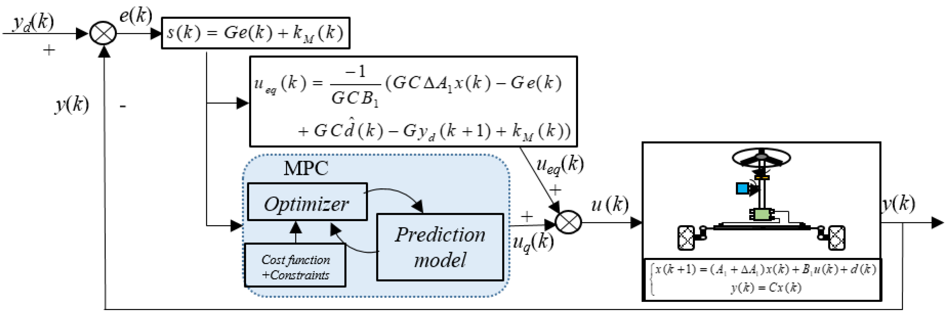
2.3. SMPC Controller Design

In this section, we improve the performance of SMC systems by using SMC and MPC together to handle the non-linearities and disturbances existing in the system. Although MPC’s rolling optimization is not globally optimal control, its objective function can achieve suboptimal solutions in the predicted time domain satisfying constraints [22], and it can compensate for system uncertainties and disturbances in a timely manner, and has better results in dealing with system hysteresis [23,24,25,26]. After we have determined the sliding mode hyperplane, we start to solve the sliding mode generation problem for the sliding mode hyperplane and the system arriving at the hyperplane in the predicted time domain. To solve both of these problems, we need to first determine the control inputs $u(k)$ to the system. As shown in Figure 4, the MPC part is used to process online and obtain a locally optimal state solution $u_q(k)$ for the system under the constraint that s converges to zero, thus achieving a system output that reaches the vicinity of the sliding mode plane. Equivalent control is then used to smooth the system state to the sliding mode.

2.3.1. Controller Design

The discrete sliding mode controller input $u(k)$ contains two components, the equivalent control input $u_{eq}(k)$ (linear state feedback control) and the non-linear control term $u_q(k)$.

$$u(k)=u_{eq}(k)+u_q(k)$$

(20)

Substitute Equation (20) and Equation (18) into Equation (15)

$$s(k+1)=s(k)+GC{B}_1{u}_q(k)+GCd(k)-GC\widehat{d}(k)$$

(21)

Express Equation (21) according to Equation (17) as

$$s(k+1)=s(k)+GC{B}_1{u}_q(k)+GC(d(k)-d(k-1))$$

(22)

Assuming that $\left|d(k)-d(k-1)\right|$ in Equation (22) is bounded

$$\begin{array}{l}\Delta d(k)=d(k)-d(k-1)={\displaystyle {\int }_0^t{e}^{At}f((k+1)t-T)d_T}-{\displaystyle {\int }_0^t{e}^{At}f(kt-T)d_T}={\displaystyle {\int }_0^t{e}^{At}{\displaystyle {\int }_{kt-T}^{(k+1)t-T}\dot{f}(\upsilon )d_{\upsilon }}{d}_T}\\ \to \left|{\displaystyle {\int }_0^t{e}^{At}{\displaystyle {\int }_{kt-T}^{(k+1)t-T}\dot{f}(\upsilon )d_{\upsilon }}{d}_T}\right|\le R\end{array}$$

$s(k+1)$ in Equation (22) represents the next step in the prediction of the sliding mode dynamics $s(k)$. The state prediction of $s(k)$ by this formula gives as follows.

$$\left\{\begin{array}{c}s(k+1)=s\left(k\right)+GC{B}_1{u}_q\left(k\right)+GC\Delta d\left(k\right)\\ s(k+2)=s\left(k\right)+GC{B}_1{u}_q\left(k\right)+GC{B}_1{u}_q(k+1)+GC\Delta d\left(k\right)+GC\Delta d(k+1)\\ s(k+3)=s\left(k\right)+GC{B}_1{u}_q\left(k\right)+GC{B}_1{u}_q(k+1)+GC{B}_1{u}_q(k+2)+GC\Delta d\left(k\right)+GC\Delta d(k+1)+GC\Delta d(k+2)\\ s(k+4)=s\left(k\right)+GC{B}_1{u}_q\left(k\right)+GC{B}_1{u}_q(k+1)+GC{B}_1{u}_q(k+2)+GC{B}_1{u}_q(k+3)+GC\Delta d\left(k\right)+GC\Delta d(k+1)+GC\Delta d(k+2)+GC\Delta d(k+3)\\ ⋮\\ s\left(k+N_c\right)=s\left(k\right)+GC{B}_1{u}_q\left(k\right)+GC{B}_1{u}_q(k+1)+GC{B}_1{u}_q(k+2)\cdots GC{B}_1{u}_q\left(k+N_c-1\right)+GC\Delta d\left(k\right)+GC\Delta d(k+1)+GC\Delta d(k+2)\cdots GC\Delta d\left(k+N_c-1\right)\\ ⋮\\ s\left(k+N_p\right)=s\left(k\right)+GC{B}_1{u}_q\left(k\right)+\cdots +\left(N_p-N_c+1\right)GC{B}_1{u}_q\left(k+N_c-1\right)+GC\Delta d\left(k\right)+\cdots +GC\Delta d\left(k+N_p-1\right)\end{array}\right.$$

Therefore

$$\begin{array}{l}s(k+q)=s(k)+GC{B}_1{u}_q(k)+\cdots +(N_p-N_c+1)GC{B}_1{u}_q(k+N_c-1)\\ \begin{array}{ccc}& & \end{array}+GC\Delta d(k)+\cdots +GC\Delta d(k+N_p-1)\end{array}$$

(23)

where $N_p$ is the prediction horizon and $N_c$ is the control horizon, the prediction function can be expressed in matrix form as

$$\left[\begin{array}{c}s(k+1)\\ s(k+2)\\ ⋮\\ s\left(k+N_c\right)\\ ⋮\\ s\left(k+N_p\right)\end{array}\right]=\left[\begin{array}{c}s\left(k\right)\\ s\left(k\right)\\ ⋮\\ s\left(k\right)\\ ⋮\\ s\left(k\right)\end{array}\right]+\left[\begin{array}{cccc}GC{B}_1& 0& \cdots & 0\\ GC{B}_1& GC{B}_1& \cdots & ⋮\\ ⋮& ⋮& \ddots & GC{B}_1\\ ⋮& ⋮& \ddots & ⋮\\ GC{B}_1& GC{B}_1& \cdots & \left(N_p-N_c+1\right)GC{B}_1\end{array}\right]\times \left[\begin{array}{c}{u}_q\left(k\right)\\ u_q(k+1)\\ ⋮\\ u_q\left(k+N_c-1\right)\end{array}\right]+\left[\begin{array}{cccccc}GC& 0& \cdots & & & 0\\ GC& GC& & & & \\ GC& GC& GC& \cdots & & \\ & & & \ddots & & ⋮\\ ⋮& ⋮& & & \ddots & 0\\ GC& GC& & \cdots & GC& GC\end{array}\right]\left[\begin{array}{c}\Delta d\left(k\right)\\ \Delta d(k+1)\\ ⋮\\ \Delta d\left(k+N_c-1\right)\\ ⋮\\ \Delta d\left(k+N_p-1\right)\end{array}\right]$$

(24)

Express Equation (24) as

$$S(k)={{\rm I}}_{s}s(k)+B_{GC{B}_1}{U}_q(k)+D_{GC}\Delta D(k)$$

(25)

where

$$\begin{gathered} {{\rm I}}_s=\left[\begin{array}{c}I\\ I\\ ⋮\\ I\\ ⋮\\ I\end{array}\right];B_{GC{B}_1}=\left[\begin{array}{cccc}GC{B}_1& 0& \cdots & 0\\ ⋮& GC{B}_1& \cdots & ⋮\\ ⋮& ⋮& \ddots & GC{B}_1\\ ⋮& ⋮& \ddots & ⋮\\ GC{B}_1& GC{B}_1& \cdots & (N_p-N_c+1)GC{B}_1\end{array}\right];U_q(k)=\left[\begin{array}{c}{u}_q(k)\\ u_q(k+1)\\ ⋮\\ u_q(k+N_c-1)\end{array}\right]; \\ {D}_{GC}=\left[\begin{array}{cccccc}GC& 0& \cdots & & & 0\\ GC& GC& & & & \\ GC& GC& GC& \cdots & & \\ & & & \ddots & & ⋮\\ ⋮& ⋮& & & \ddots & 0\\ GC& GC& & \cdots & GC& GC\end{array}\right];\Delta D(k)=\left[\begin{array}{c}\Delta d(k)\\ \Delta d(k+1)\\ ⋮\\ \Delta d(k+N_c-1)\\ ⋮\\ \Delta d(k+N_p-1)\end{array}\right] \end{gathered}$$

2.3.2. Optimal Solution

In practice, the control increment $\Delta u_q(k)$ of the automatic tractor steering system is unknown, while the control increment can only be solved by means of a suitable optimization objective to obtain a suitable control sequence in the control time domain. According to the relevant definitions in the literature [27,28],

$$\left\{\begin{array}{c}J={\left({\mathrm{R}}_s-Y\right)}^T({\mathrm{R}}_s-Y)+\Delta U^{T}R\Delta U\\ {\mathrm{R}}_s^T=\left[\begin{array}{ccc}1& \cdots & 1_{N_p}\end{array}\right]r(k)\end{array}\right.$$

(26)

Here, the first term indicates the magnitude of the error between the predicted output and the set input signal, and the second term indicates the value of $\Delta U$ when the objective function J is as small as possible. R is the weight matrix and the final minimum objective function is established as shown below.

$$J(k)=S^T(k)S(k)+\Delta U_q^T(k)R\Delta U_q(k)$$

(27)

2.3.3. Design of Constraints

The first term of the objective function indicates the tracking performance of the system for the SMC output term, i.e., the MPC input term signal, the second term indicates the smoothness requirement for the control quantity, the tractor needs to constrain the state quantity and control quantity of the system when the tractor is actually operating, R is the weight matrix.

Control volume constraints:

$$u_{q\min }(k)\le u_q(k)\le u_{q\max }(k)$$

(28)

Control of incremental constraints:

$$\Delta u_{q\min }(k)\le \Delta u_q(k)\le \Delta u_{q\max }(k)$$

(29)

Denote $u_q(k)$ and $\Delta u_q(k)$ by the relationship between control quantities and control increments as $\Delta u_q(k)=u_q(k)-u_q(k-1)$. Then, $u_q(k)=u_q(k-1)+\Delta u_q(k)$; write the state prediction for $u_q(k)$ as

$$\left\{\begin{array}{c}{u}_q(k)=u_q(k-1)+\Delta u_q(k)\\ u_q(k+1)=u_q(k)+\Delta u_q(k+1)=u_q(k-1)+\Delta u_q(k)+\Delta u_q(k+1)\\ ⋮\\ u_q(k+N_c-1)=u_q(k+N_c-2)+\Delta u_q(k+N_c-1)=u_q(k-1)+\Delta u_q(k)+\cdots +\Delta u_q(k+N_c-1)\end{array}\right.$$

(30)

Then, Equation (30) is written in the form of a state-space equation

$$\left[\begin{array}{c}{u}_q(k)\\ u_q(k+1)\\ ⋮\\ u_q(k+N_c-1)\end{array}\right]=\left[\begin{array}{c}{u}_q(k-1)\\ u_q(k-1)\\ ⋮\\ u_q(k-1)\end{array}\right]+\left[\begin{array}{cccc}I& 0& \cdots & 0\\ I& I& 0& 0\\ ⋮& 0& \ddots & ⋮\\ I& I& \cdots & I\end{array}\right]\left[\begin{array}{c}\Delta u_q(k)\\ \Delta u_q(k+1)\\ ⋮\\ \Delta u_q(k+N_c-1)\end{array}\right]$$

(31)

Denote this as

$$U_q(k){=\mathrm{I}}_u{u}_q(k-1){+\mathrm{L}}_U\Delta U_q(k)$$

(32)

We represent the constraint $\Delta U_q(k)$ as a parametric linearization inequality, and SMPC is converted to solve the optimal problem using Quadratic Programming (QP) [27], such that the input signal $\Delta U_q(k)={\left[\begin{array}{cccc}\Delta u_q(k)& \Delta u_q(k+1)& \cdots & \Delta u_q(k+N_c-1)\end{array}\right]}^T$, subject to satisfying the system constraints, is made to slip the modal term $S(k)\to 0$ by step $N_c$. The constraint relationship between $U_q(k)$ and $\Delta U_q(k)$ is expressed according to the relationship between the control volume constraint (28) and the control increment constraint (29) as

$$U_{q\min }(k)\le {\mathrm{I}}_u{u}_q(k-1){+\mathrm{L}}_U\Delta U_q(k)=U_q(k)\le U_{q\max }(k)$$

(33)

$$\Delta U_{q\min }(k)\le \Delta U_q(k)\le \Delta U_{q\max }(k)$$

(34)

Using the inequality constraint is expressed as

$$\left\{\begin{array}{l}-{\mathrm{L}}_U\Delta U_q(k)\le -U_{q\min }(k)+{\mathrm{I}}_u{u}_q(k-1)\\ {\mathrm{L}}_U\Delta U_q(k)\le U_{q\max }(k)-{\mathrm{I}}_u{u}_q(k-1)\\ -\Delta U_q(k)\le -\Delta U_{q\min }(k)\\ \Delta U_q(k)\le \Delta U_{q\max }(k)\end{array}\right.$$

(35)

Then, the system constraints are expressed in matrix form as

$$\left[\begin{array}{c}-{\mathrm{L}}_U\\ {\mathrm{L}}_U\\ -I\\ I\end{array}\right]\Delta U_q(k)\le \left[\begin{array}{c}-U_{q\min }(k)+{\mathrm{I}}_u{u}_q(k-1)\\ U_{q\max }(k)-{\mathrm{I}}_u{u}_q(k-1)\\ -\Delta U_{q\min }(k)\\ \Delta U_{q\max }(k)\end{array}\right]$$

(36)

Further expressed in the form of a constraint equation

$$L_{U,I}\times \Delta U_q(k)-U_{U,\Delta }\le 0$$

(37)

where

$$L_{U,I}=\left[\begin{array}{c}-{\mathrm{L}}_U\\ \begin{array}{l}{\mathrm{L}}_U\\ -I\\ I\end{array}\end{array}\right];\hspace{1em}{U}_{U,\Delta }=\left[\begin{array}{c}-U_{q\min }(k)+{\mathrm{I}}_u{u}_q(k-1)\\ U_{q\max }(k)-{\mathrm{I}}_u{u}_q(k-1)\\ -\Delta U_{q\min }(k)\\ \Delta U_{q\max }(k)\end{array}\right];$$

$\Delta U_q(k)$ subject to the constraints above can be expressed in terms of the cost function as

$$\begin{array}{l}J(k)=S^T(k)S(k)+\Delta U_q^T(k)R\Delta U_q(k)=\\ \left[\begin{array}{cccccc}s(k+1)& s(k+2)& \cdots & s(k+N_c)& \cdots & s(k+N_p)\end{array}\right]\left[\begin{array}{c}s(k+1)\\ s(k+2)\\ ⋮\\ s(k+N_c)\\ ⋮\\ s(k+N_p)\end{array}\right]+\\ \lambda [\begin{array}{cccc}\Delta u_q(k)& \Delta u_q(k+1)& \cdots & \Delta u_q(k+N_c-1)\end{array}]\left[\begin{array}{c}\Delta u_q(k)\\ \Delta u_q(k+1)\\ ⋮\\ \Delta u_q(k+N_c-1)\end{array}\right]\\ ={\displaystyle \sum _{i=1}^{N_p}s{(k+i)}^2+}\lambda {\displaystyle \sum _{j=1}^{N_c}\Delta u_q{(k+j-1)}^2}\end{array}$$

(38)

where $\lambda$ is the weighting matrix used to limit the partial control effort. Considering that the system model is changing in real-time, the linear constraint for the optimization link is solved by the Lagrange multiplier method in order to find the minimum value of J(k). The Lagrange multiplier method is a method for finding the extreme value of a multi-variate function when the variables are subject to one or more constraints. The Lagrange multiplier method [28,29] is introduced to solve for the constraints by constructing an incremental extensive function.

The minimum value of the cost function of the system of Lagrange multiplier $\lambda (k)$ introduced into the pending Lagrange multiplier vector is expressed as

$$\min J(k)=S^T(k)S(k)+\Delta U_q^T(k)R\Delta U_q(k)+{\lambda }^T(L_{U,I}\times \Delta U_q(k)-U_{U,\Delta })$$

(39)

This converts the optimization problem of a system containing constraints into a problem of solving the extreme value of a system of equations using the classical variational method (the variables are not subject to any constraints). It is easy to see that the value of (38) subject to the equality constraints $L_{U,I}\times \Delta U_q(k)-U_{U,\Delta }=0$ being satisfied is the same as the original objective function.

The value of the disturbance term $\Delta D(k)$ in Equation (25) $S(k)={{\rm I}}_{s}s(k)+B_{GC{B}_1}{U}_q(k)+D_{GC}\Delta D(k)$ is unknown and is estimated by prediction

$$\Delta \widehat{D}(k)=\left[\begin{array}{c}\Delta d(k)\\ \Delta d(k+1)\\ ⋮\\ \Delta d(k+N_c-1)\\ ⋮\\ \Delta d(k+N_p-1)\end{array}\right]$$

(40)

When the system enters the sliding modal zone (i.e., when the value of the cost function is minimal), the cost function needs to satisfy the following conditions.

$$\left\{\begin{array}{c}\frac{dJ}{d\lambda }=0\\ \frac{dJ}{d{u}_q}=0\end{array}\right.$$

(41)

By solving Equation (41) we get

$$\begin{array}{l}{\lambda }^{\ast }=-{[L_{U,I}{({2L_U}^T{B}_{GC{B}_1}{}^T{B}_{GC{B}_1}{L}_U+2R)}^{-1}{L_{U,I}}^T]}^{-1}[U_{U,\Delta }+{({L_U}^T{B_{GC{B}_1}}^T{B}_{GC{B}_1}{L}_U+R)}^{-1}\\ \hspace{1em}\hspace{1em}{L}_U{}^T{B}_{GC{B}_1}{}^T(s(k)+B_{GC{B}_1}{\mathrm{I}}_u{u}_q(k-1)+D_{GC}\Delta \widehat{D}(k))]\\ \Delta U_q(k)=-{(L_U{}^T{B}_{GC{B}_1}{}^T{B}_{GC{B}_1}{L}_U+R)}^{-1}[L_{U,I}{}^T{\lambda }^{\ast }+L_U{}^T{B}_{GC{B}_1}{}^T(s(k)\\ \hspace{1em}\hspace{1em}+B_{GC{B}_1}{\mathrm{I}}_u{u}_q(k-1)+D_{GC}\Delta \widehat{D}(k))]\end{array}$$

(42)

Then, according to Equation (32), $u_q(k)$ is the first element of $U_q(k)$, i.e., $u_q(k)=\left[\begin{array}{cccc}1& 0& \cdots & 0\end{array}\right]{(\mathrm{I}}_u{u}_q(k-1){+\mathrm{L}}_U\Delta U_q(k))$, $\Delta u_q(k)$ is the first element of $\Delta U_q(k)$, then the total control behavior of the steering system SMPC is expressed as

$$\begin{array}{l}u(k)=u_{eq}(k)+u_q(k)=u_{eq}(k)+\left[\begin{array}{cccc}1& 0& \cdots & 0\end{array}\right]({\mathrm{I}}_u{u}_q(k-1){+\mathrm{L}}_U\Delta U_q(k))=\\ \frac{-1}{GC{B}_1}\left[GC\Delta {\widehat{A}}_{1}x(k)-Ge(k)+GC\widehat{d}(k)-G{y}_d(k+1)+k_M(k)\right]+\\ \left[\begin{array}{cccc}1& 0& \cdots & 0\end{array}\right]({\mathrm{I}}_u{u}_q(k-1)-L_U{(L_U{}^T{B}_{GC{B}_1}{}^T{B}_{GC{B}_1}{L}_U+R)}^{-1}[L_{U,I}{}^T{\lambda }^{\ast }+L_U{}^T{B}_{GC{B}_1}{}^T(s(k)\\ +B_{GC{B}_1}{\mathrm{I}}_u{u}_q(k-1)+D_{GC}\Delta \widehat{D}(k))])\end{array}$$

(43)

2.4. SMPC-Based Steering System Stability Analysis

In this section, we analyze the stability of the system according to the definition of sliding mode variable structure control [30].

We consider that the discrete model of the steering system satisfies the property of arriving near the boundary of the sliding mode surface, as in the switching surface of Figure 5 [31]. Since the discrete system sliding mode control can only produce quasi-sliding mode control, rather than ideal sliding mode control. Normally the quasi-sliding control system movement consists of a phase of movement outside the sliding surface ($A\to B$) and a phase of movement near and along the sliding surface ($B\to C$) as shown in Figure 6. Thus, in the quasi-sliding mode region.

$$-\Delta \le S(k+1)\le \Delta$$

(44)

In the above equation, $2\Delta$ is the width of the switching band of the sliding mode control system.

In the vicinity of the switching surface, the switching band near the sliding surface is defined as

$$S_{\Delta }=\left\{\left.k\in R^n\right|-\Delta <S(k)<\Delta \right\}$$

(45)

Then, in the vicinity of the switching zone there is

$$\left\{\begin{array}{c}-\Delta \le S(k+1)<S(k)\begin{array}{c}\end{array}for\begin{array}{c}\end{array}S(k)>\Delta \\ S(k)=0\\ S(k)<S(k+1)\le \Delta \begin{array}{c}\end{array}for\begin{array}{c}\end{array}S(k)<-\Delta \end{array}\right.$$

(46)

Considering the discrete quasi-sliding mode control arrival condition when the sliding mode function needs to satisfy $\left|S(k+1)\right|\le \left|S(k)\right|$, then due to $\left|S(k)\right|\le \Delta$, we get $\left|S(k+1)\right|\le \Delta$. Additionally, according to the definition of sliding mode control of discrete systems in the paper [32], it is known that the system is stable.

According to Equation (13), substituting the first term of Equation (43) into Equation (15) yields

$$\begin{array}{c}s(k+1)=GC\left(A_1+\Delta A_1\right)x\left(k\right)+GCd\left(k\right)-G{y}_d(k+1)+k_M(k+1)+GC{B}_{1}u\left(k\right)=\hfill \\ GC\left(A_1+\Delta A_1\right)x\left(k\right)+GCd\left(k\right)-G{y}_d(k+1)+k_M(k+1)+GC{B}_1\frac{-1}{GC{B}_1}\hfill \\ \left[GC\Delta {\widehat{A}}_{1}x\left(k\right)-Ge\left(k\right)+GC\widehat{d}\left(k\right)-G{y}_d(k+1)+k_M\left(k\right)\right]+GC{B}_1\left(I_u{u}_q(k-1)\right.\hfill \\ \left.-L_U{\left(L_U{}^T{B}_{GC{B}_1}{}^T{B}_{GCB}{L}_U+R\right)}^{-1}\left[L_{U,I}{}^T{\lambda }^{\ast }+L_U{}^T{B}_{GC{B}_1}^T\left(s\left(k\right)+B_{GCB}{I}_u{u}_q(k-1)+D_{GC}\Delta \widehat{D}\left(k\right)\right)\right]\right)\hfill \\ =GC{A}_{1}x\left(k\right)+GC\left(\Delta A_1-\Delta \widehat{A_1}\right)x\left(k\right)+GCd\left(k\right)-GC\widehat{d}\left(k\right)+k_M(k+1)+Ge\left(k\right)-k_M\left(k\right)+GC{B}_1\left(I_u{u}_q(k-1)\right.\hfill \\ \left.-L_U{\left(L_U{}^T{B}_{GC{B}_1}{}^T{B}_{GCB}{L}_U+R\right)}^{-1}\left[L_{U,I}{}^T{\lambda }^{\ast }+L_U{}^T{B}_{GC{B}_1}{}^T\left(s\left(k\right)+B_{GCB}{I}_u{u}_q(k-1)+D_{GC}\Delta \widehat{D}\left(k\right)\right)\right]\right)\hfill \end{array}$$

(47)

$s(k+1)$ is the first element of $S(k)$. To reduce the computational effort, when the values of R and ${\lambda }^{\ast }$ are 0

$$\begin{array}{l}S(k)=s(k+1)=GC{A}_{1}x(k)+GC(\Delta A_1-\Delta {\widehat{A}}_1)x(k)+GCd(k)-GC\widehat{d}(k)\\ +k_M(k+1)+Ge(k)-k_M(k)+GC{B}_1({\mathrm{I}}_u{u}_q(k-1)-L_U{(L_U{}^T{B}_{GC{B}_1}{}^T{B}_{GC{B}_1}{L}_U)}^{-1}\\ [L_U{}^T{B}_{GC{B}_1}{}^T(s(k)+B_{GC{B}_1}{\mathrm{I}}_u{u}_q(k-1)+D_{GC}\Delta \widehat{D}(k))])\\ =GC(\Delta A_1-\Delta {\widehat{A}}_1)x(k)+GC(d(k)-2d(k-1)+d(k-2))\end{array}$$

(48)

In the above equation, since both $\Delta A_1$ and $\Delta {\widehat{A}}_1$ are bounded, and by the definition of sliding mode control

$$\left\{\begin{array}{c}1/2GC(\Delta A_{1\min }-\Delta A_{1\max })x(k)\le GC(\Delta A_1-\Delta {\widehat{A}}_1)\le 1/2GC(\Delta A_{1\max }-\Delta A_{1\min })x(k)\\ GC(d(k)-2d(k-1)+d(k-2))\le GC\Delta \\ \left|\Delta d(k)\right|=\left|d(k)-d(k-1)\right|\le R\end{array}\right.$$

(49)

So

$$\begin{gathered} \left|S(k+1)\right|\le \left|S(k)\right|=\left|s(k+1)\right|\le \Delta \\ \left|S(k+1)\right|\le \left|S(k)\right|=\left|s(k+1)\right|\le \left|GC(\frac{(\Delta A_{1\max }-\Delta A_{1\min })x(k)}{2}+2R)\right|\le \Delta \end{gathered}$$

(50)

The above calculations lead to the conclusion that the SMPC control system designed for the steering system is a stable system that effectively suppresses and compensates for system parameter disturbances and external disturbances.

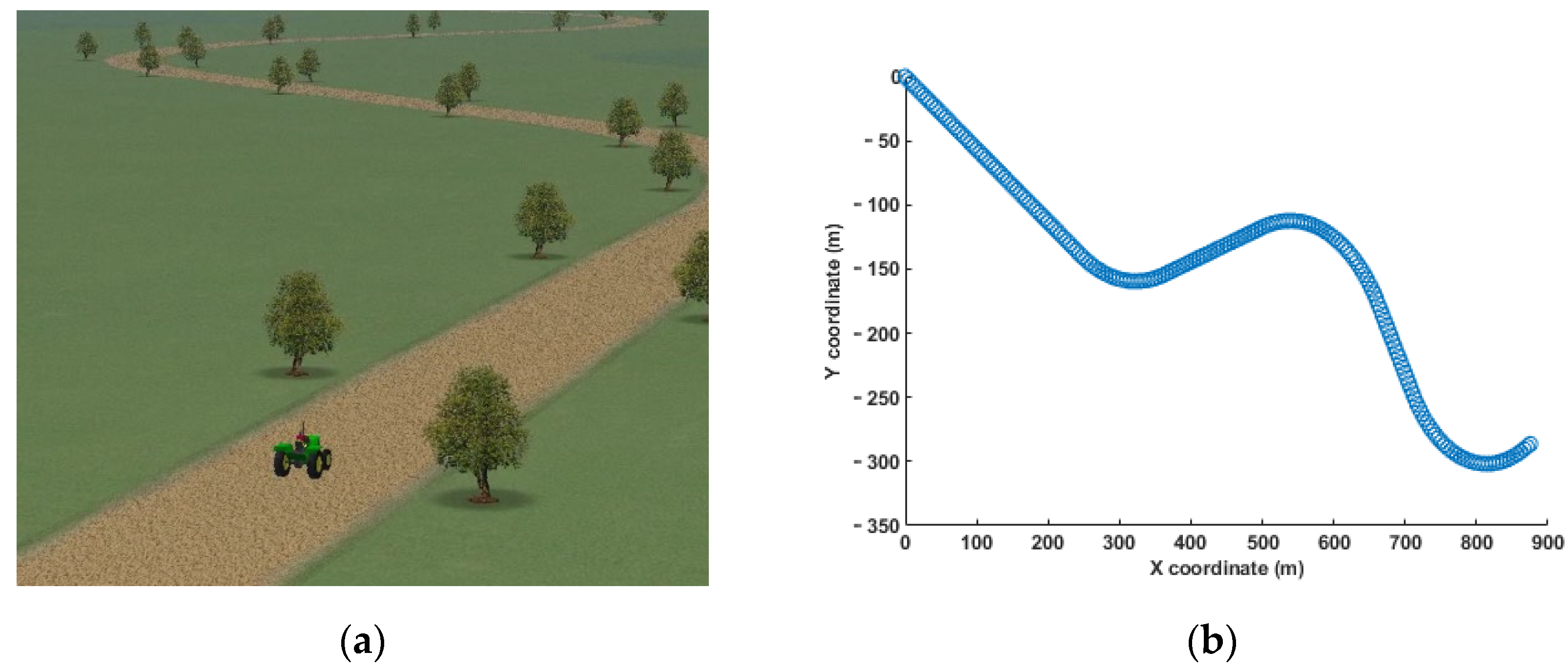
2.5. Validation of Simulation Results

To demonstrate the effectiveness of the proposed control algorithm, the steering system SMC and SMPC controllers were modelled by MATLAB/Simulink, respectively. The state vector of the system is $x(k)={[\begin{array}{cc}x1(k)& x2(k)\end{array}]}^T$. In order to verify the immunity of the system to disturbances, a disturbance (step signal, initial value: 1; final value: 0) is added at 2 s. When the SMC controller is simulated, the results are shown in Figure 7 and Figure 8.

Additionally, for the SMPC control strategy simulation, the results are obtained as shown in Figure 9.

As can be seen in Figure 8 and Figure 9, the SMPC is able to handle the chattering of the SMC very well, mainly because it has the advantage of feedback correction and receding horizon optimization of the MPC controller, which compensates for the chattering caused by the SMC control switching. In addition, the SMPC quickly returns to a stable state after an external disturbance input at 2 s, proving that it can effectively handle external disturbances.

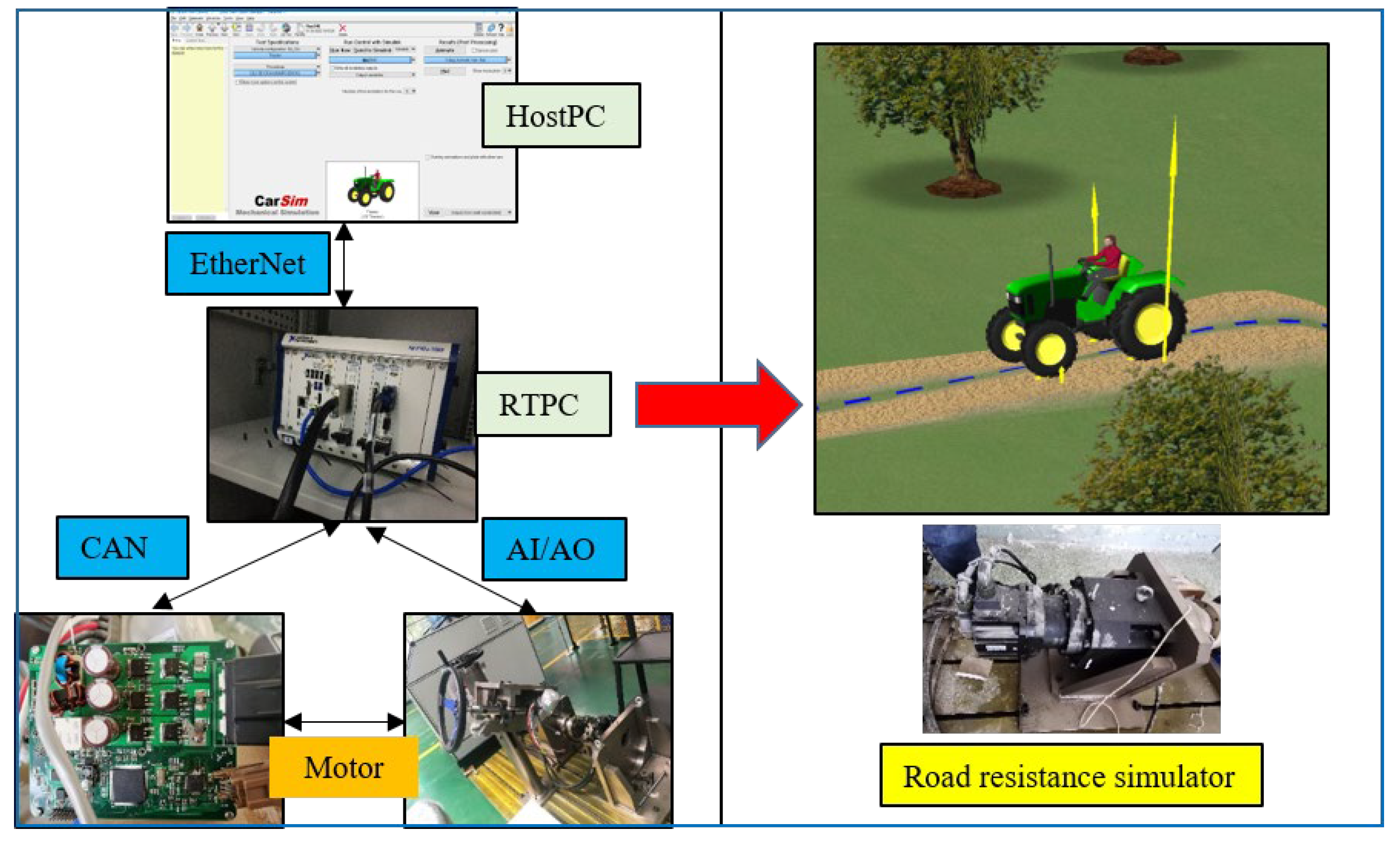
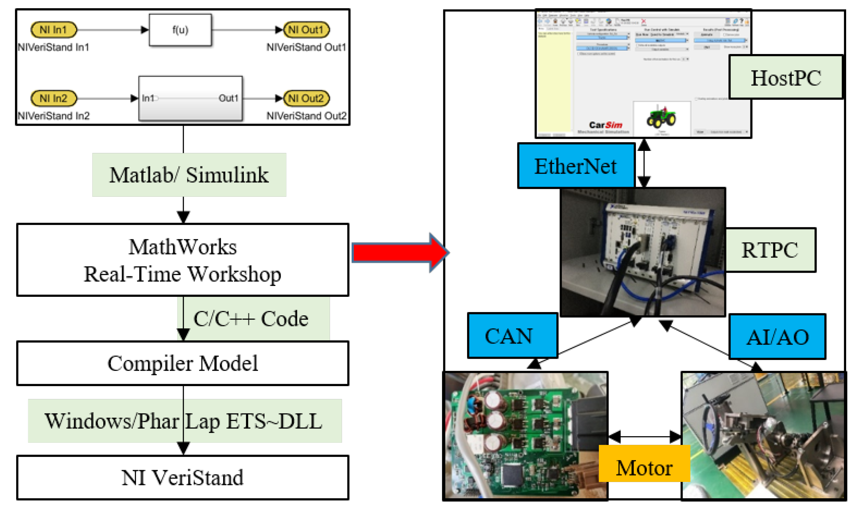
2.6. Test Verification

In this section, to better validate the steering system SMPC control strategy, the control algorithm simulation platform was built through a joint CarSim/Simulink simulation [33,34], and the steering control system was tested in hardware in the loop on a steering test rig based on NI’s PXI measurement and control platform. The hardware-in-the-loop (HIL) tests can be carried out in place of a real vehicle under certain conditions, replacing the driver’s operation in some extreme sections to prevent accidents, and some experimental data can be easily interacted with via the host computer. The following settings are made for the CarSim math model: Time step 0.001 (s), Freq 1000 (Hz); Output file: Time step 0.01(s), Freq 100 (Hz); Integration method: AM-2 (2 updates per step).

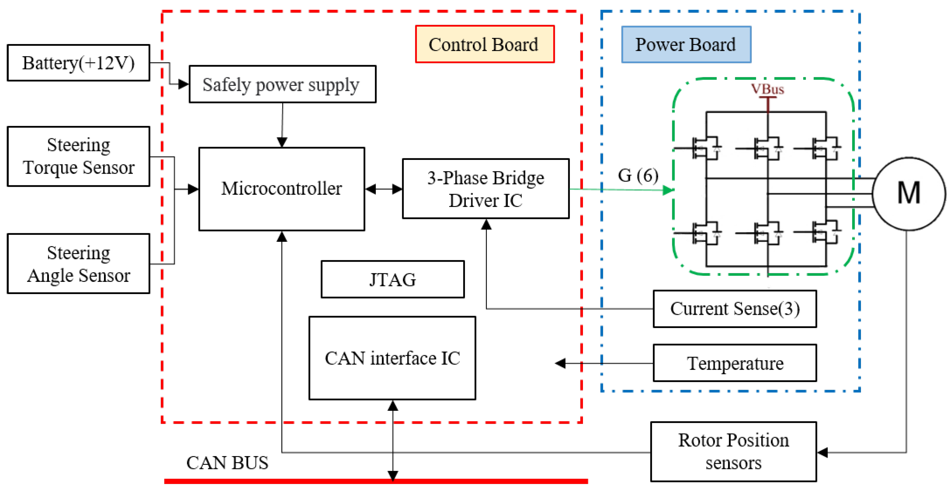
Introduction to Test Benches

The test platform is shown in Figure 10, this experiment platform is mainly comprised of power supply system, hydraulic station, steering resistance motor, PMSM drive board, permanent magnet synchronous motor (PMSM) and steering power transfer system, hydraulic steering valve, NI-PXI real-time platform (chassis: NI PXIe-1082, controller: PXIe-8840 Quad-Core, modules: PXIe-6363DAQ Card (AI: −10 V~+10 V, 16 bits, 2 MSample/s; AO: −10 V~+10 V, 16 bits, 2.86 MSample/s), PXI-8512 CAN Card, PXIe-6612 Timing Card). The specific functions of the steering system equipment are described below. The power supply system provides electrical power to the permanent magnet synchronous motor and its drive board, the hydraulic station provides steering hydraulic power to the steering valve, the EPS works with the hydraulic power steering system under the steering column to provide total steering assistance, and the road resistance simulation uses the steering load motor (Panasonic AC SERVO MOTOR, 5 KW, 23.9 N.m) to provide simulated steering resistance. The PXI-8512 CAN Card communicates with and controls the steering PMSM motor controller [35] and acquires the steering angle torque sensor and motor operating current signals. The CarSim vehicle system calculates the front wheel steering resistance based on the cornering signal, vehicle model and road conditions, then outputs an analogue voltage signal to the steering load motor via the PXIe-6363 DAQ Card’s AO channel to provide steering resistance and collects the torque signal from the entire steering system and the hydraulic fluid pressure and flow signals from the hydraulic power steering system via the AI channel.

The control strategy of the system is implemented on the PXI platform from NI. The general workflow is shown in Figure 11. The control algorithm model is established through the MATLAB/Simulink software and LabVIEW Model Interface Toolkit (MIT) of the upper computer and the DLL file is generated and imported to the LabVIEW software platform, and CarSim through the Phar Lap ETS system of the PXI platform. The specific vehicle dynamics model runs on the NI-PXI real-time system and is communicated and controlled by the PXI CAN card with the steering PMSM motor drive board. The AI channel of the PXI DAQ Card is used to collect the hydraulic pressure flow signals and the AO channel generates the corresponding voltage signal to the road simulation motor to achieve the steering resistance loading. The performance of the control algorithm is evaluated by the output of the steering test bench system and the performance parameters.

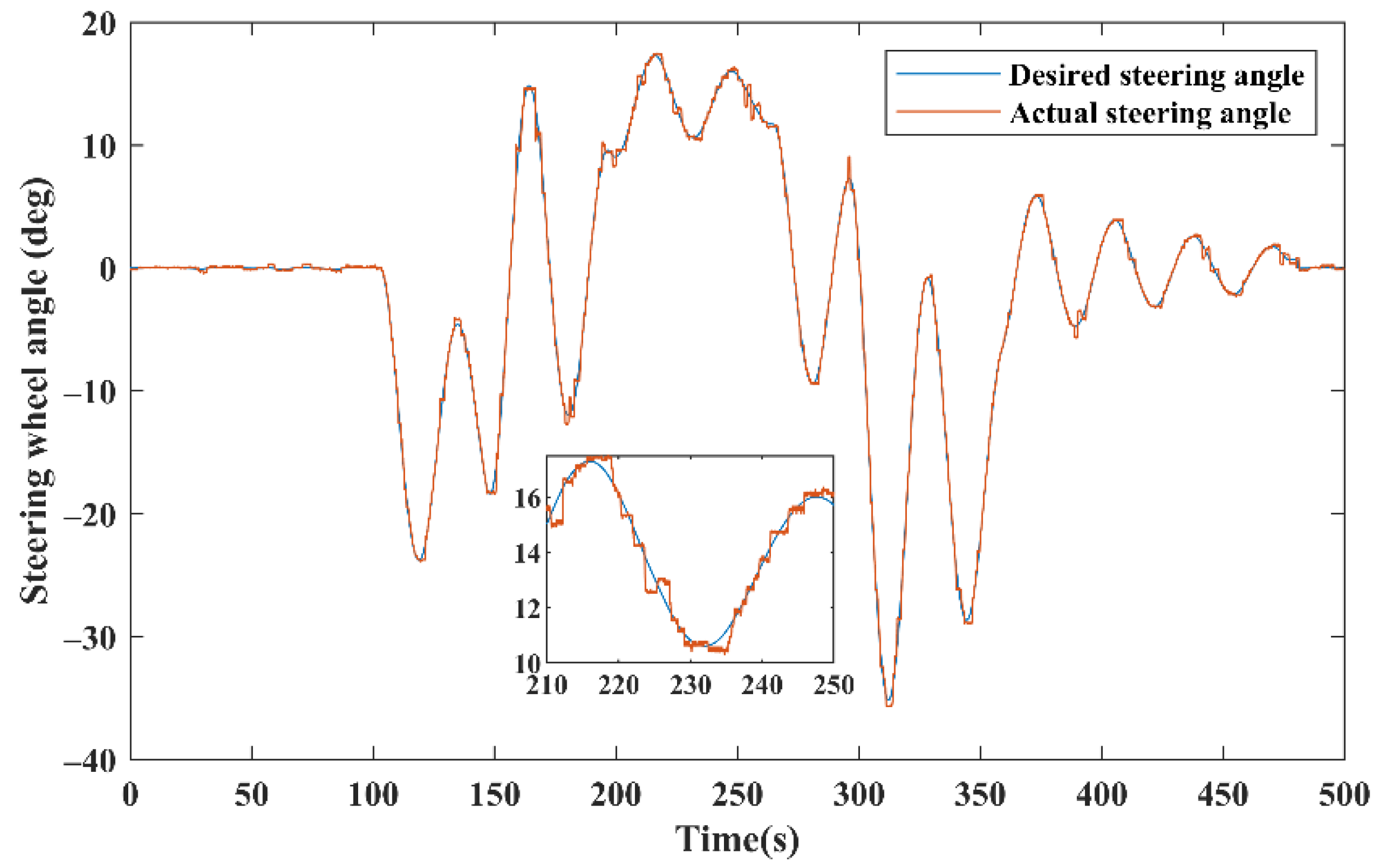
3. Results and Discussion

Analysis and Discussion of Experimental Results

The steering system angle tracking was investigated when the tractor speed was set to 10 km/h. The driving road coordinates were as shown in Figure 12, and the tire–road friction coefficient of the soil road was 0.5.

The steering angle tracking test is carried out when the tractor is travelling over flat terrain and the relevant test parameters are shown in Figure 13, Figure 14, Figure 15 and Figure 16 below.

When a tractor is in the field, the steering system is subject to external environmental disturbances, such as changes in terrain. Due to the terrain, the tractor will generate a lateral force component, which will cause some disturbance to the steering system when it changes. A simulation road environment was built to better verify the stability of the steering system under changing terrain. The relevant road parameters are set as shown in Figure 17 below, with the road gradient being relatively flat at the start (0–120 m) and end (1080–1200 m) positions, while three ramps occur in the middle position, with a right-leaning road in the middle section of the route (at approximately 600–840 m) and left-leaning ramps at the 360 m and 1000 m positions.

The results shown in Figure 18, Figure 19, Figure 20 and Figure 21 were obtained for steering system target angle tracking under the effect of road gradient.

Comparative analysis of target steering angle tracking (Figure 13 vs. Figure 18): when the tractor travels along a fixed route, on flat terrain and road slope conditions, the trend of the change in the angle is more or less the same. However, at 100 s, there is a certain amount of jitter due to the terrain, while at approximately 120, 230 and 320 s, the expected front wheel angle changes significantly due to the road gradient and road curvature, but the expected front wheel angle is much smaller than in flat terrain under the effect of the terrain gradient and the steering system can accurately and quickly track the target angle in both terrains.

Motor current analysis (Figure 14 vs. Figure 19): when the tractor travels along a fixed route, on flat terrain and road slope conditions, the current change trend is more or less the same, and the target angle tracking compared to the steering change amplitude is relatively large at the moment the current change amplitude is larger, indicating that the current and steering motor angle change is associated with the actual phenomenon observed. By tracking the current in different terrains, we can found the desired steering angle in curved road sections so that the terrain gradient is smaller than the desired turning angle in flat terrain, mainly because the additional lateral force component generated when driving on road gradients is used to balance the steering resistance.

Hydraulic steering system oil pressure analysis (Figure 15 vs. Figure 20): when the tractor travels along a fixed route, the hydraulic station provides 2.5 MPa of stable flow of hydraulic oil to the hydraulic steering system; as shown in Figure 15 and Figure 20, the steering system rotation caused by hydraulic oil pressure change fluctuations are more obvious—the amplitude of the curve is greater than when driving along a straight route. The steering system is influenced by the slope of the road; in the curved position of the ramp driving section, the hydraulic fluid change amplitude is smaller than in the flat terrain, and the main actor is the ramp role of additional lateral force components used to balance the steering resistance, reducing the demand for steering assistance, so that the hydraulic fluid in can achieve target corner tracking control at smaller pressure.

Steering system steering resistance torque analysis (Figure 16 vs. Figure 21): when the tractor travels along a fixed route, the steering load motor (used for road resistance simulation) and the steering system interact to produce a resistance torque; as shown in Figure 16 and Figure 21, when the vehicle travels along a flat terrain compared to a hilly terrain, the driving resistance torque trends are approximately the same, and straight road changes fluctuate little, while curve steering road fluctuations change significantly. At 300–350 s, it can be seen that when the steering angle changes, the steering torque also changes. However, due to the terrain, the change in torque is much smaller compared to on flat terrain.

4. Conclusions

To improve the operational performance of the automatic tractor steering system, this paper proposes an electro-hydraulic coupled steering (EHCPS) system scheme combining EPS and HPS, and investigates the control strategy of the system. To improve the anti-disturbance capability of the steering system, the SMPC control strategy is proposed to address the problem of jitter and vibration in the SMC-controlled sliding mode surface switching, and feedback correction and receding horizon optimization are introduced into the SMC control. It is demonstrated through simulations and hardware-in-the-loop tests that the control strategy can effectively handle external disturbances and provide accurate control of the steering system while satisfying the constraints. The steering system has only been verified on the test stand due to the limitations of the conditions, and there are certain gaps compared to the actual operation in the field. Therefore, subsequent studies will be considered to carry out retrofitting studies on the real vehicle platform and to better refine the control strategy in the real operating environment.

References

1. Abroshan, M.; Taiebat, M.; Goodarzi, A. Automatic steering control in tractor semi-trailer vehicles for low-speed maneuverability enhancement. Proc. Inst. Mech. Eng. 2016, 231, 83–102. [Google Scholar] [CrossRef]
2. Liu, J.Y.; Tan, J.Q.; Mao, E.R. Proportional directional valve based automatic steering system for tractors. Front. Inf. Technol. Electron. Eng. 2016, 17, 458–464. [Google Scholar] [CrossRef]
3. Huynh, V.; Smith, R.; Kwok, N.M.; Katupitiya, J. Anonlinear PI and back stepping-based controller for tractor-steerable trailers influenced by slip. In Proceedings of the 2012 IEEE International Conference on Robotics and Automation (ICRA), Saint Paul, MN, USA, 14–18 May 2012; pp. 245–252. [Google Scholar]
4. Fang, H. Automatic Guidance of Farm Vehicles in Presence of Sliding Effects; Universite Blaise Pascal: Aubière, France, 2004. [Google Scholar]
5. Javad, T.; Xu, W.; Stanley, L.; Jay, K. A sliding mode controller with a nonlinear disturbance observer for a farm vehicle operating in the presence of wheel slip. In Proceedings of the 2013 IEEE/ASME International Conference on Advanced Intelligent Mechatronics, Wollongong, NSW, Australia, 9–12 July 2013. [Google Scholar]
6. Massera, F.C.; Wolf, D.F. Driver assistance controller for tire saturation avoidance up to the limits of handling. In Proceedings of the 2015 3rd Brazilian Symposium on Robotics (LARS-SBR), Uberlandia, Brazil, 29–31 October 2015. [Google Scholar]
7. Meiling, W.; Zhen, W.; Yi, Y.; Mengyin, F. Model predictive control for ugv trajectory tracking based on dynamic model. In Proceedings of the 2016 IEEE International Conference on Information and Automation, Ningbo, China, 1–3 August 2016. [Google Scholar]
8. Keviczkv, T.; Falcone, P.; Borrelli, E. Predictive control approach to autonomous vehicle steering. In Proceedings of the 2006 American Control Conference, Minneapolis, MN, USA, 14–16 June 2006. [Google Scholar]
9. Wang, G.D.; Liu, L.; Qing, G. Integrated Path tracking control of steering and braking based on holistic MPC. IFAC Pap. Line 2021, 54, 45–50. [Google Scholar] [CrossRef]
10. Huang, X.Y. Robust weighted gain-scheduling H∞ vehicle lateral motion control with considerations of steering system backlash-type hysteresis. IEEE Trans. Control Syst. Technol. 2014, 22, 1740–1753. [Google Scholar] [CrossRef]
11. Zhao, J.M.; Jie, M.; Zhang, L.J. Passivity-based sliding mode predictive control of discrete-time singular systems with time-varying delay. In Proceedings of the 2011 International Conference on Consumer Electronics, Communications and Networks, Xianning, China, 16–18 April 2011. [Google Scholar]
12. Kim, S.H.; Shin, M.C.; Chu, C.N. Development of EHPS motor speed map using HILS system. IEEE Trans. Veh. Technol. 2013, 62, 1553–1567. [Google Scholar] [CrossRef]
13. Miao, H.Q.; Diao, P.S.; Xu, G.F. Research on decoupling control for the longitudinal and lateral dynamics of a tractor considering steering delay. Sci. Rep. 2022, 12, 1–23. [Google Scholar] [CrossRef]
14. Dannöhl, C.; Müller, S.; Ulbrich, H. H∞-control of a rack-assisted electric power steering system. Veh. Syst. Dyn. 2012, 50, 527–544. [Google Scholar] [CrossRef]
15. Zhao, W.Z.; Zhou, X.C.; Wang, C.Y. Energy analysis and optimization design of vehicle electro-hydraulic compound steering system. Appl. Energy 2019, 255, 113713. [Google Scholar] [CrossRef]
16. Sharp, R.S.; Granger, R. On car steering torques at parking speeds. Proc. Inst. Mech. Eng. Part D J. Automob. Eng. 2003, 217, 87–96. [Google Scholar] [CrossRef]
17. Kim, W.; Son, Y.S.; Chung, C.C. Torque overlay-based robust steering wheel angle control of electrical power steering for a lane-keeping system of automated vehicles. IEEE Trans. Veh. Technol. 2016, 65, 4379–4392. [Google Scholar] [CrossRef]
18. Wu, J.; Zhang, J.; Liu, Y.; He, X.K. Adaptive control of PMSM servo system for steering-by-wire system with disturbances observation. IEEE Trans. Transp. Electrif. 2015, 8, 2015–2028. [Google Scholar] [CrossRef]
19. Xu, Q.S.; Li, Y.M. Micro-/Nanopositioning using model predictive output integral discrete sliding mode control. IEEE Trans. Ind. Electron. 2012, 59, 1161–1170. [Google Scholar] [CrossRef]
20. Young, K.D.; Utkin, V.I.; Ozguner, U. A control engineer’s guide to sliding mode control. IEEE Trans. Control Syst. Technol. 1999, 7, 328–342. [Google Scholar] [CrossRef] [Green Version]
21. Furuta, K. Sliding mode control of a discrete system. Syst. Control Lett. 1990, 14, 145–152. [Google Scholar] [CrossRef]
22. Hyunsik, N.; Wansik, C.; Changsun, A. Model predictive control for evasive steering of an autonomous vehicle. Int. J. Automot. Technol. 2019, 20, 1033–1042. [Google Scholar]
23. Wang, Y.; Hou, M. Model-free adaptive integral terminal sliding mode predictive control for a class of discrete-time nonlinear systems. ISA Trans. 2019, 93, 209–217. [Google Scholar] [CrossRef]
24. Bao, C.J.; Feng, J.W.; Wu, J. Model predictive control of steering torque in shared driving of autonomous vehicles. Sci. Prog. 2020, 103, 1–22. [Google Scholar] [CrossRef]
25. Shi, G.B.; Zhou, Q.; Wang, S. High robust control strategy for electro-hydraulic hybrid steering system in unmanned mode. Trans. Chin. Soc. Agric. Mach. 2019, 50, 395–402. [Google Scholar]
26. Wu, J.; Tian, Y.; Walker, P. Attenuation reference model based adaptive speed control tactic for automatic steering system. Mech. Syst. Signal Process. 2021, 156, 107631. [Google Scholar] [CrossRef]
27. Kuhne, F.; Fetter, W. Model predictive control of a mobile robot using linearizaton. Proc. Mechatron. Robot. 2004, 4, 525–530. [Google Scholar]
28. Wang, L.P. Model Predictive Control System Design and Implementation Using MATLAB®; Springer: London, UK, 2009; pp. 43–86. [Google Scholar]
29. Erkan, K.; Erkan, K.; Herman, R. Distributed nonlinear model predictive control of an autonomous tractor–trailer system. Mechatronics 2014, 24, 926–933. [Google Scholar]
30. Yongsoon, E.; Jung, H.K.; Kwangsoo, K. Discrete-time variable structure controller with a decoupled disturbance compensator and its application to a CNC servomechanism. IEEE Trans. Control Syst. Technol. 1999, 7, 414–423. [Google Scholar] [CrossRef]
31. Hung, J.Y.; Gao, W.; Hung, J.C. Variable structure control: A survey. IEEE Trans. Ind. Electron. 1993, 40, 2–22. [Google Scholar] [CrossRef] [Green Version]
32. Bartoszewicz, A. Discrete-time quasi-sliding mode control strategies. IEEE Trans. Ind. Electron. 1998, 45, 633–637. [Google Scholar] [CrossRef]
33. Xie, B.; Wang, S.; Wu, X.H. Design and hardware-in-the-loop test of a coupled drive system for electric tractor. Biosyst. Eng. 2022, 216, 165–185. [Google Scholar] [CrossRef]
34. Jeon, C.-W.; Kim, H.-J. An entry-exit path planner for an autonomous tractor in a paddy field. Comput. Electron. Agric. 2021, 191, 106548. [Google Scholar] [CrossRef]
35. Rohrer, R.A.; Pitla, S.K.; Luck, J.D. Tractor CAN bus interface tools and application development for real-time data analysis. Comput. Electron. Agric. 2019, 163, 104847. [Google Scholar] [CrossRef]
Figure 1. Functional diagram of the automatic steering system.
Agriculture 12 02091 g001
Figure 2. Structure of electro-hydraulic coupling power steering system.
Agriculture 12 02091 g002
Figure 3. EPS system PMSM motor control board operating schematic.
Agriculture 12 02091 g003
Figure 4. Control structure of the SMPC controller.
Agriculture 12 02091 g004
Figure 5. Switching surface characteristics.
Agriculture 12 02091 g005
Figure 6. Regions defined by the switching logic.
Agriculture 12 02091 g006
Figure 7. Graph of system state vector changes (SMC and SMPC).
Agriculture 12 02091 g007
Figure 8. Plot of s and u versus time (SMC).
Agriculture 12 02091 g008
Figure 9. Plot of s and u versus time (SMPC).
Agriculture 12 02091 g009
Figure 10. Hardware-in-the-loop simulation testbed.
Agriculture 12 02091 g010
Figure 11. Implementation of the control strategy.
Agriculture 12 02091 g011
Figure 12. Driving road scenario (a) and coordinates (b).
Agriculture 12 02091 g012
Figure 13. The steering angle tracking effect when driving on flat terrain.
Agriculture 12 02091 g013
Figure 14. EPS motor current detection values when driving on flat terrain.
Agriculture 12 02091 g014
Figure 15. Test value of hydraulic oil pressure on flat terrain.
Agriculture 12 02091 g015
Figure 16. Resistance torque detection values when driving on flat terrain.
Agriculture 12 02091 g016
Figure 17. Schematic diagram of the change in road topography height.
Agriculture 12 02091 g017
Figure 18. Steering angle tracking effect when driving on sloping terrain.
Agriculture 12 02091 g018
Figure 19. Current tracking effect when driving on sloping terrain.
Agriculture 12 02091 g019
Figure 20. Oil pressure detection diagram for sloping terrain.
Agriculture 12 02091 g020
Figure 21. Resistance torque detection values when driving on sloping terrain.
Agriculture 12 02091 g021
Publisher’s Note: MDPI stays neutral with regard to jurisdictional claims in published maps and institutional affiliations.