Article

Modeling and Application of Temporal Correlation of Grain Temperature during Grain Storage

1
College of Agricultural Equipment Engineering, Henan University of Science and Technology, Luoyang 471000, China
2
College of Biology and Agricultural Engineering, Jilin University, Changchun 130022, China
*
Author to whom correspondence should be addressed.
Agriculture 2022, 12(11), 1883; https://doi.org/10.3390/agriculture12111883
Submission received: 28 September 2022 / Revised: 28 October 2022 / Accepted: 5 November 2022 / Published: 9 November 2022

Abstract

:
Temperature measurement system malfunction and sensor failure in grain storage warehouses can lead to missing grain temperature data on some days. Missing data is not conducive to the monitoring of grain storage conditions. This paper establishes mathematical models of temporal correlation coefficients of grain temperature and storage time in different planes, and analyzes the influence of storage state change on grain temperature correlation. The historical grain situation data for about one year were selected from 27 flat grain storage warehouses distributed in the second to seventh grain storage ecological zones in China. In addition, correlation coefficients of grain temperature were then calculated on the XOY, XOZ and YOZ planes of each warehouse. During this process, the time interval included 1, 7, 14, 21, 28, 35, 42, 49, 56, 63 and 70 days, meaning that the correlation coefficients between the grain temperature on the day and the grain temperature after storage for 1, 7, 14, 21, 28, 35, 42, 49, 56, 63 and 70 days were calculated. Next, the correlation coefficients from the same time intervals and planes in each warehouse were sequentially connected to form arrays of correlation coefficients. Then, the 3σ-threshold setting methods and DBSCAN (density-based spatial clustering of applications with noise) method were used to analyze the correlation coefficients those arrays. According to the results, we set the correlation coefficient thresholds for each plane (XOY, XOZ and YOZ planes) at each time interval. The models were then established regarding the correlation coefficient thresholds and storage time intervals. Subsequently, the sum of squares for error (SSE), coefficient of determination (R2), and root mean square error (RMSE) were chosen to evaluate the models, with the results showing that the effect of the model established by the threshold set by the 3σ-setting method, with SSE, R2 and RMSE of 0.056, 0.9771 and 0.0748, respectively, was better than the model established using the DBSCAN method. Finally, the correlation coefficients of grain temperatures with empty warehouse, new grain addition, aeration and self-heating were analyzed. The results show that the four modes in a certain time interval (e.g., 30 days) does not meet the correlation coefficient threshold during normal storage. The result can provide a theoretical basis for grain storage condition detection when grain temperature data is intermittently missing.

1. Introduction

Detection of grain condition is an effective measure for ensuring the security of grain storage. All state-owned grain depots in China have a grain condition measurement system installed to monitor grain conditions changes [1]. On the one hand, effective detection and analysis of grain conditions can avoid condensation, mildew [2,3,4] and other conditions that affect grain quality, and can also prevent illegal behaviors affecting grain quantity [5,6,7]. On the other hand, accurate analysis of historical grain conditions can provide clues for the inspection work of government staff for grain conditions, and therefore the analysis of grain storage conditions is of great significance for the management and audit system of grain depots, so as to ensure the quantity and quality safety of stored grain.
Grain condition detection systems can provide grain condition data for assisting grain management personnel to analyze grain condition at each grain depot. At present, grain condition detection systems can detect indicators such as temperature, humidity, pest insects, moisture, temperature, humidity, and gas concentrations inside and outside the granary [8]. On the basis of the detected grain condition data, some scholars have established mathematical models coupled with a certain factor or multiple factors [9,10], and then used the models to predict and analyze the temperature, humidity, and other indicators of grain bulk. Some scholars have used CFD and other simulation software to simulate and analyze the changing process of temperature field, humidity field, and other fields in grain bulk [11,12,13,14,15]. These provide theoretical models for grain condition analysis. Others have studied the coupling relationship between the temperature field, humidity field [16,17], pressure field [18], biological field [19], and other fields in the grain bulk, and proposed a method of multifield coupling for grain condition analysis. This method was preliminarily shown to be able to realize the analysis and judgment of grain condition with respect to aspects that affect grain quality, such as condensation [16,17], mildew, etc., and was able to perform online monitoring and analysis of grain quantity [18]. The studies mentioned above perform the detection, prediction and judgment of grain quality and quantity by analyzing grain storage condition data and establishing models. However, there has been research focusing on the analysis of historical grain condition data to propose methods for grain storage supervision and management on-site.
In our research group, some studies were carried out on how to use historical grain temperature data (which are part of the grain data) to provide clues for storage supervision and management on-site. The main research areas include three aspects: (a) the use of RGB or HSV color and other color features of temperature field contour maps to monitor the quantity of stored grain quantity [20]; (b) the monitoring of grain storage conditions on the basis of the temporal and spatial correlation of grain temperature [21]; (c) grain storage conditions were analyzed and judged by the statistical characteristic of grain temperature change [22,23,24]. These studies mainly detected the historical grain storage conditions from the two aspects of temperature field cloud map and statistical characteristics on the adjacent two days, and realized the detection and classification of grain storage condition changes. The methods mentioned above are based on the continuity of historical grain temperature data collected at the adjacent time. When the historical grain temperature data are missing for more than one week due to system malfunction, sensor failure, etc., the grain temperature data at those times are difficult to obtain on the basis of interpolation. Thus, the above research methods are difficult to adapt to this situation. Therefore, it is of certain significance to study how to use the grain temperature data in which there are long stretches of time with missing data to analyze and detect abnormal changes in grain storage conditions. Missing data regarding grain temperature in the time domain indicate that the time interval between two groups of grain temperature data is long, and can also be expressed as a long period of storage without the collection of data.
To verify that the temporal correlation of grain temperature in each plane can be used to detect abnormal grain conditions with missing grain temperature data in the time domain, the following research was performed. In this context, the objectives of this research were: (1) to analyze and set the correlation coefficient of the grain temperature threshold for each plane stored for different days; (2) to establish models for the correlation coefficient of the grain temperature threshold; (3) to verify that the abnormal changes in grain temperature can be detected within a certain time when employing the threshold set by the model, no matter what grain temperature data may be missing during this time.

2. Data and Methods

2.1. Grain Temperature Data Collection and Processing

2.1.1. Data Collection

The data source for this paper is historical grain temperature data obtained using electronic temperature detection systems during grain storage in granaries located in different provinces. Following pre-processing, the grain temperature data for about one year in 27 flat granaries with complete data (data continuous storage time ≥ 12 months) were selected for analysis. Among them, ten, nine and eight granaries were used to store rice, corn and wheat, respectively, and were distributed in Henan, Anhui, Hubei, Fujian, Sichuan, Guizhou, Jiangsu, Jilin, Heilongjiang and other provinces, representing a distribution from the second to the seventh ecological grain storage regions in China.
The grain in the flat granaries had been loaded into them between 2017 and 2018. subsequently, the grain was to be stored in the granary for about 2–4 years. During the storage process, the temperature sensors installed in the grain bulk (Figure 1) measure grain temperature 1–2 times per week. All of these grain temperature data are stored in the server of the grain depots. The staff of the grain depots judge the grain storage condition using the grain temperature data in addition to other grain condition data on the basis of their experience. If the grain storage conditions change, the granary will be ventilated or fumigated in time to ensure the safety of the grain.

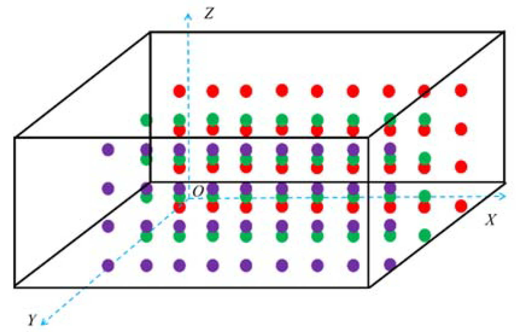
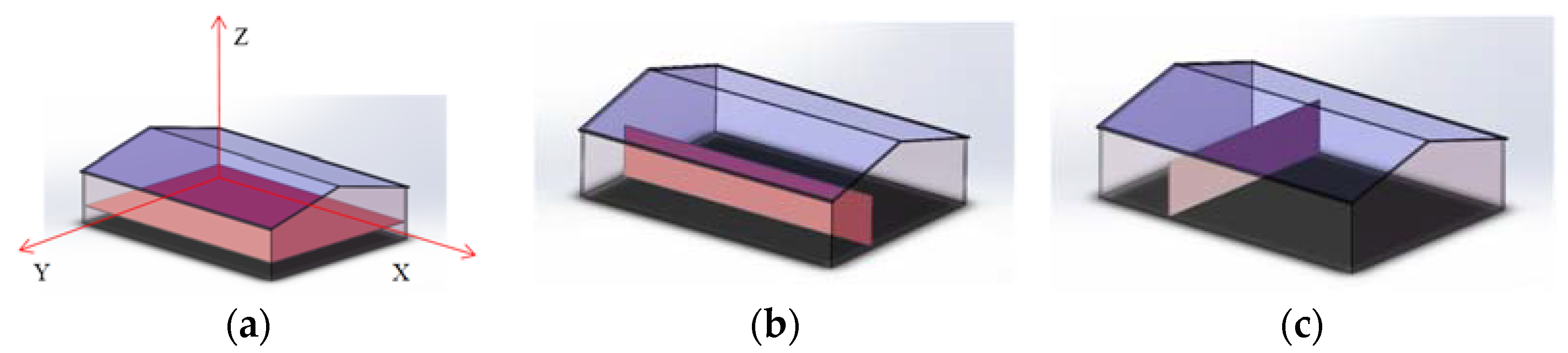
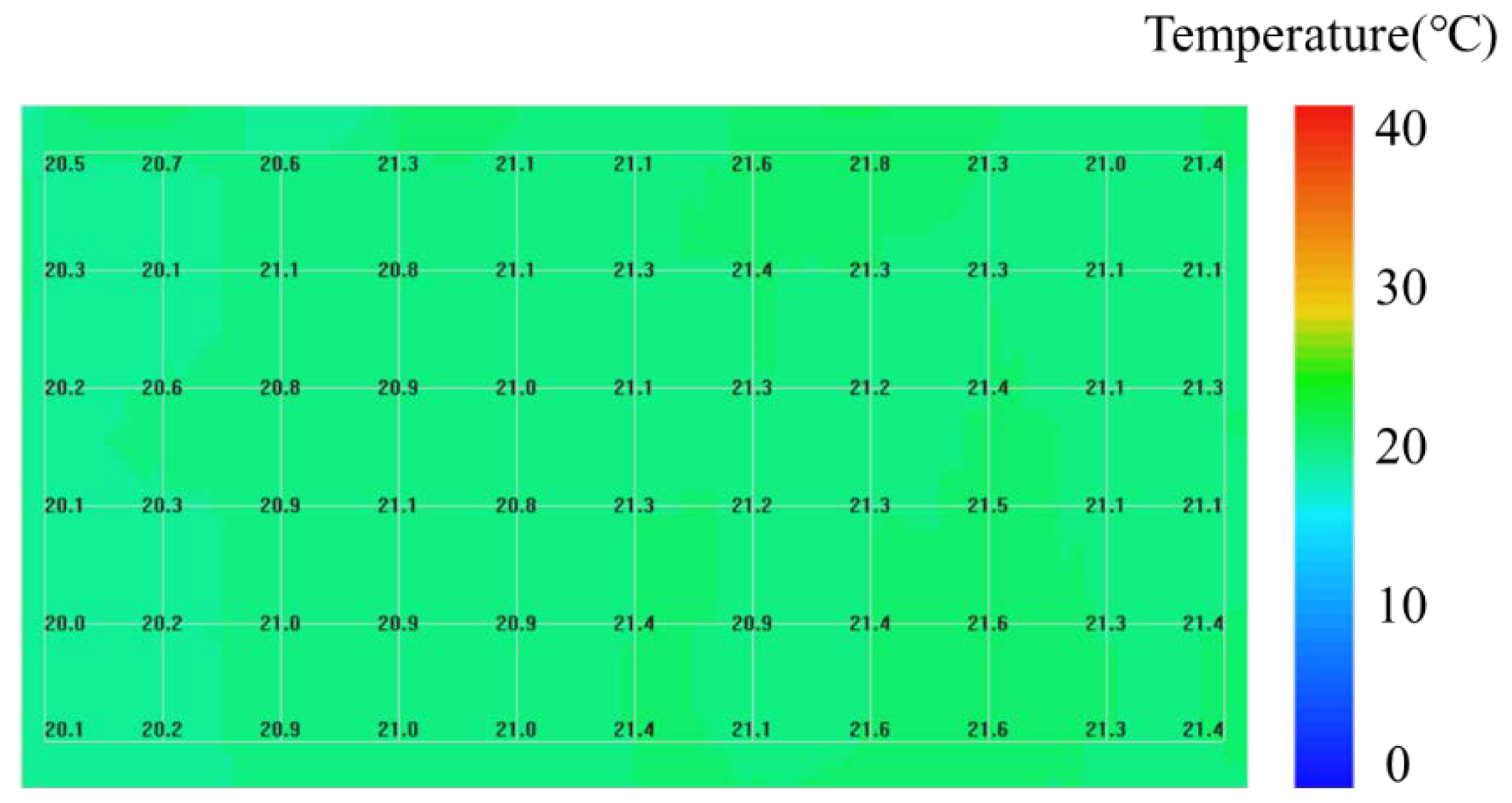
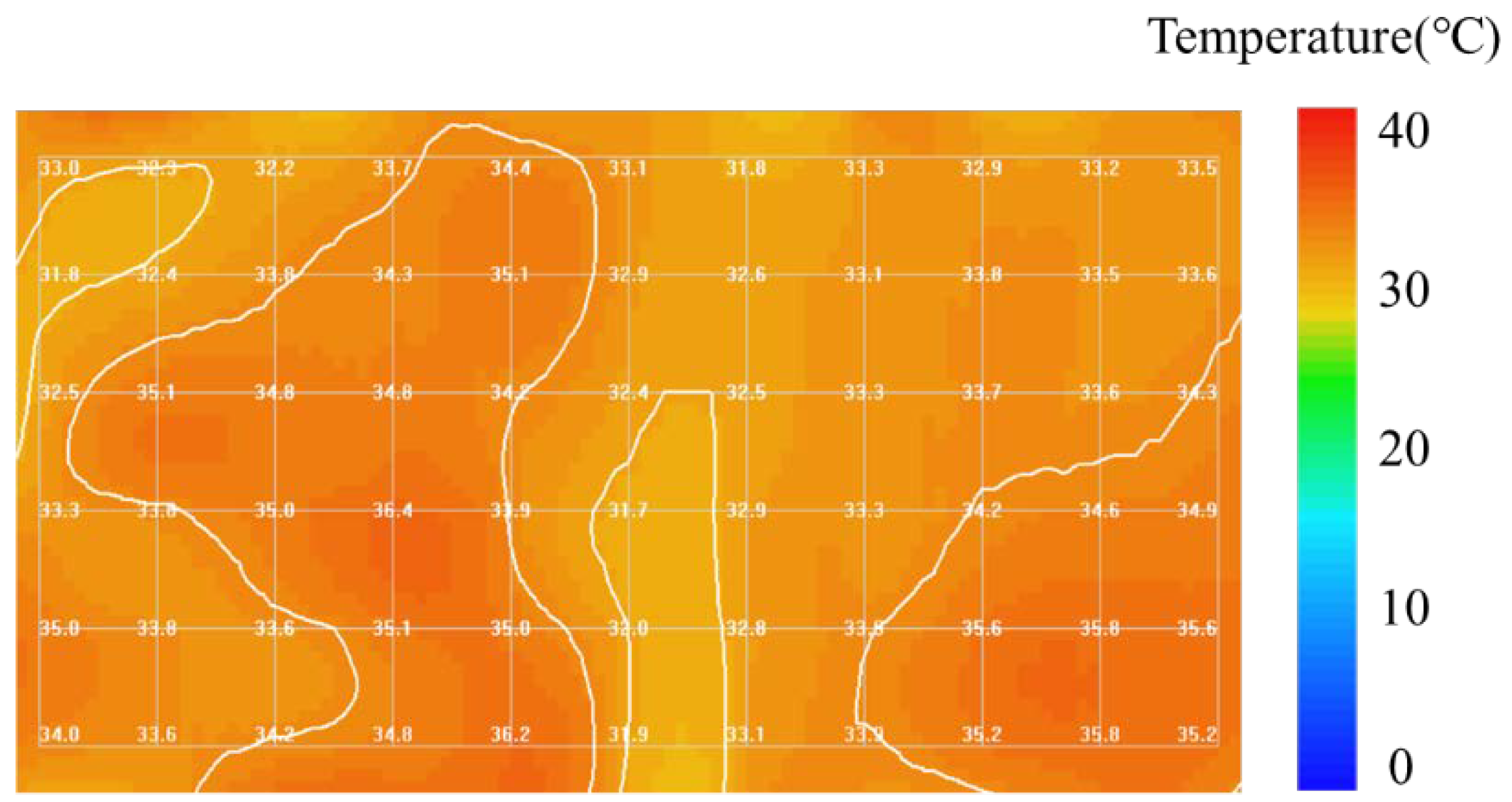
2.1.2. Grain Temperature Plane Composition

A coordinate system is established to define the location of each temperature sensor in the warehouse under consideration (Figure 2a). Depending on the coordinates, a three-dimensional matrix of temperature measurement points was established. There are n, m, and l temperature measurement points in the X, Y, and Z directions of the matrix, respectively. The coordinates (x, y, z) of each temperature measurement point in the granary are expressed as (i, j, k), and the temperature at this point is Tijk, where 0 < in, 0 < jm, 0 < kl (i, j, k are integers). The temperature sensors form three planes that are parallel to the XOY, XOZ, and YOZ planes, respectively, namely, a plane parallel to XOY (referred to as the XOY plane), a plane parallel to XOZ (referred to as the XOZ plane) and a plane parallel to YOZ (referred to as the YOZ plane), as shown in Figure 2. Among the granaries selected, l = 4, m = 4~10, and n = 6~15.

2.1.3. Grain Temperature Data Preprocessing

All grain temperature datasets are preprocessed to remove obvious outliers caused by sensor failures and software malfunction. These outliers typically appear as abnormal values (beyond the physically possible temperature range), such as 888 °C and −85 °C, or simply a non-numerical error code, depending on the type of hardware and software used. The outliers are simply replaced by the average temperatures for that day. In this paper, grain temperature was collected 1–3 times each week. The missing grain temperature was supplemented by linear interpolation based on the grain temperature data obtained for the days before and after. The above methods were used to preprocess the grain temperature data to ensure a dataset of grain temperature every day. Subsequently, in order to facilitate the analysis of different grain storage states, the dynamic grain inventory analysis system (V1.0, Tianjin Minglun Electronic Technology Co., Ltd., Tianjin, China) was used to convert the above grain temperature data into the temperature field cloud maps.

2.2. Research Methods

2.2.1. Time Correlation Calculation Method for Plane Grain Temperature

Grain bulk has poor thermal conductivity, and small daily average temperature changes at each temperature measurement point. Thus, the temperature and humidity information at the same location in the grain bulk at similar times should be related [25,26]. The correlation characteristic of temperature in the time domain is called the time correlation, which has nothing to do with the time for which the grain has been stored, and is less affected by the location of the grain bulk. With reference to the formula of Pearson’s correlation coefficient [27,28], the cross-correlation coefficient Rz of grain temperature in the XOY plane can be obtained using Equation (1). Additionally, the correlation coefficients Ry and Rx of the grain temperature in the XOZ plane and the YOZ plane can be obtained. During storage, the grain temperature is usually collected 1~2 times a week. To more accurately analyze grain temperature data, seven days was taken as a cycle within which to calculate the XOY-plane grain temperature correlation coefficient for 27 granaries over 3 months, that is, the time intervals between t1 and t2 in Equation (1) are 1, 7, 14, 21, 28, 35, 42, 49, 56, 63, 70, 77, 84, and 91 days. The lower limits of the distribution interval of the correlation coefficient of grain temperature from the first to the fourth layers are shown in Figure 3.
From Figure 3, it can be seen that the correlation coefficient of grain temperature decreased to below zero at storage times of more than 37 days. According to [21], when the correlation coefficient of grain temperature is lower than zero, the grain temperature of two groups will differ greatly. Thus, there is no point in studying grain temperature with values of correlation coefficient lower than zero. However, in order to fully study the relationship between storage time and the correlation coefficient, the grain temperature correlation coefficient at about 70 days was chosen for further analysis.
R z = i = 1 n j = 1 m ( T i j k t 1 T k t 1 ¯ ) ( T i j k t 2 T k t 2 ¯ ) i = 1 n j = 1 m ( T i j k t 1 T k t 1 ¯ ) 2 i = 1 n j = 1 m ( T i j k t 2 T k t 2 ¯ ) 2 ( k = 1 ~ l )
where Tijkt1 and Tijkt2 are the grain temperature data matrix at the time t1 and t2 of the XOY plane of the kth layer; T k t 1 ¯ and T k t 2 ¯ are the mean values of grain temperature at the time of t1 and t2 of the XOY plane of the kth layer, °C.
Ref. [21] showed that the grain temperature correlation threshold is the interval at which the distribution of the correlation coefficients is concentrated, where the upper limit of this interval is one, and the lower limit varies. The lower limit is called the correlation coefficient threshold.

2.2.2. Correlation Coefficient Preprocessing

Each temperature measurement plane corresponds to a correlation coefficient. The number of correlation coefficients in the X and Y directions is different in different granaries because of the different values of n and m. To connect the correlation coefficients of the 27 granaries in sequence, the origin of the coordinate system located at O was taken as the starting point, and the correlation coefficients of 4 planes moving continuously in the positive directions of X and Y were selected to ensure that the numbers of correlation coefficients in the X and Y directions were the same. The number of correlation coefficients in the Z direction was four, since l = 4. Correlation coefficients belonging to the same plane under the same amount of storage time were sequentially connected for each granary. Then, in this way, four sets of correlation coefficient vectors in the X, Y and Z directions were formed at each time for the 27 granaries. Taking the grain temperature on the XOY plane as an example, the correlation coefficient vectors formed in the granaries were Rz1, Rz2, Rz3, and Rz4, respectively. Rz1, Rz2, Rz3, and Rz4 represent the correlation coefficient vectors of the grain temperature in the first, second, third, and fourth XOY planes from the top layer to bottom layer, respectively. Similarly, the vectors of the correlation coefficient in the XOZ and YOZ planes are Ry = {Ry1, Ry2, Ry3, Ry4} and Rx = {Rx1, Rx2, Rx3, Rx4}, respectively. The correlation coefficients of storage for 1, 7, 14, 21, 28, 35, 42, 49, 56, 63, and 70 days are processed in the same way to form arrays.

2.2.3. Threshold Setting Method

(1)
Threshold Setting Method Based on DBSCAN Clustering
DBSCAN is a density clustering method based on the compactness of the dataset. Its core idea is to start from a certain core point and continuously expand to the density-reachable area, so as to obtain a maximized area including core points and boundary points at which the density of any two points is connected, thus obtaining a cluster category. Different groups of closely connected maximized regions compose the final clustering result [29,30]. The key parameters (ϵ, MinPts) in the DBSCAN algorithm are used to describe the tightness of the sample distribution in the neighborhood. Among them, ϵ describes the neighborhood distance threshold of a sample, and MinPts describes the threshold of the number of samples in the neighborhood, where the distance of a sample is ϵ [31,32]. The values of the clustering parameters (ϵ, MinPts) in the three planes are determined on the basis of pre-experiments. For the XOY plane, the parameter (ϵ, MinPts) is equal to (0.01, 50); for the XOZ plane and the YOZ plane, the parameter (ϵ, MinPts) is equal to (0.02, 50).
Taking the XOY plane as an example, the correlation coefficient set Rz was divided into four vectors—Rz1, Rz2, Rz3, and Rz4—for the purposes of clustering. To set the input matrix of the clustering algorithm, a constant vector of the same length (the constant is 1) was added in front of four vectors to form a matrix as the input matrix of the clustering algorithm, namely {1(x), Rz1(x)}, {1(x), Rz2(x)}, {1(x), Rz3(x)}, {1(x), Rz4(x)} (1 < xs, s represents the value of Rz1 length). Before clustering, the number of clusters k was set to two, and the criterion function is the sum of the distances of points between clusters. After the clustering had been completed, the maximum and minimum values of the ordinates in each category were taken to form threshold intervals, and the minimum value was set as the correlation coefficient threshold for the purposes of modeling analysis. The XOZ plane and the YOZ plane were handled in the same way.
(2)
3σ-Threshold-Based Setting Method
The 3σ threshold setting method calculates the mean μ and variance σ on the basis of historical data of the process parameters in their normal state. The threshold range was set to within [μ − 3σ, μ + 3σ]. On the basis of our knowledge of probability theory, the probability of falling within this range is 99.73%, and the probability of falling outside this range is only 0.27%, thus representing a low-probability event [33]. According to the above method, the thresholds of a total of 12 vectors, such as Rz1, Rz2, Rz3, Rz4, Ry1, etc., of the correlation coefficient sets of different storage times are calculated. A correlation coefficient threshold was obtained for each plane under each storage time, and the correlation coefficient threshold is modeled and analyzed below.

2.2.4. Model Building Method and Environment

The storage time was taken as the abscissa t, and the correlation coefficient threshold was set as the ordinate f(t). The Rational function in the cftool toolbox was used to model it in MATLAB (2016b, MathWorks, Natick, MA, USA). The model is shown in Equation (2). The threshold models of XOY plane, XOZ plane and YOZ plane are shown in Figure 4.
f ( t ) = p 1 × t + p 2 t + q 1  
The computer configuration used for clustering and modeling was as follows: the processor was an Intel(R) Core (TM) i3-2350M, the CPU frequency was 2.30 GHz, the memory was 4.00 GB, and the operating system was Windows 7 (64-bit). The development environment was MATLAB2016b.

2.2.5. Relevance Rating

Based on Table 1 of Pearson’s correlation coefficient grading rules [28], and the autocorrelation coefficient threshold 0.8 of flat grain temperature during normal storage in the reference [21], the flat grain temperature correlation coefficient grading rule was set as shown in Table 1.

2.2.6. Evaluation of the Model Index

To evaluate the performance of the grain temperature correlation threshold prediction model, three evaluation indicators were used in this paper: the sum of squares of error (SSE), the coefficient of determination (R2), and the root mean square error (root mean square error, RMSE). The equations of each evaluation index are shown below.
SSE = I = 1 N w I ( y I y ¯ I ) 2
R 2 = 1 I = 1 N ( y I f I ) 2 I = 1 N ( y I y ¯ ) 2
RMSE = 1 N I = 1 N ( y I f I ) 2
where f I is the predicted value; y I is the value of the correlation coefficient threshold; y ¯ is the average of correlation coefficient threshold; N is the number of correlation coefficient threshold.

3. Results and Discussion

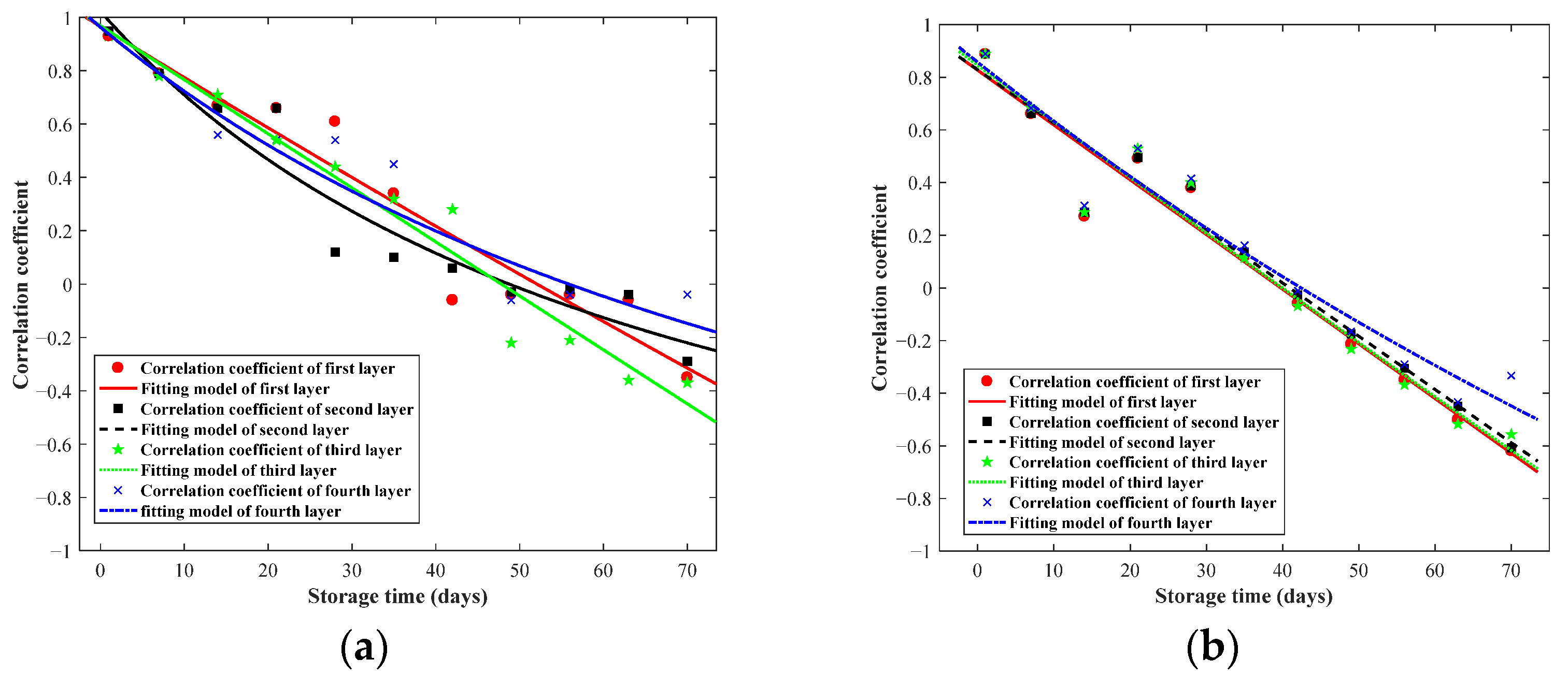
3.1. Mode of Correlation Coefficient Threshold

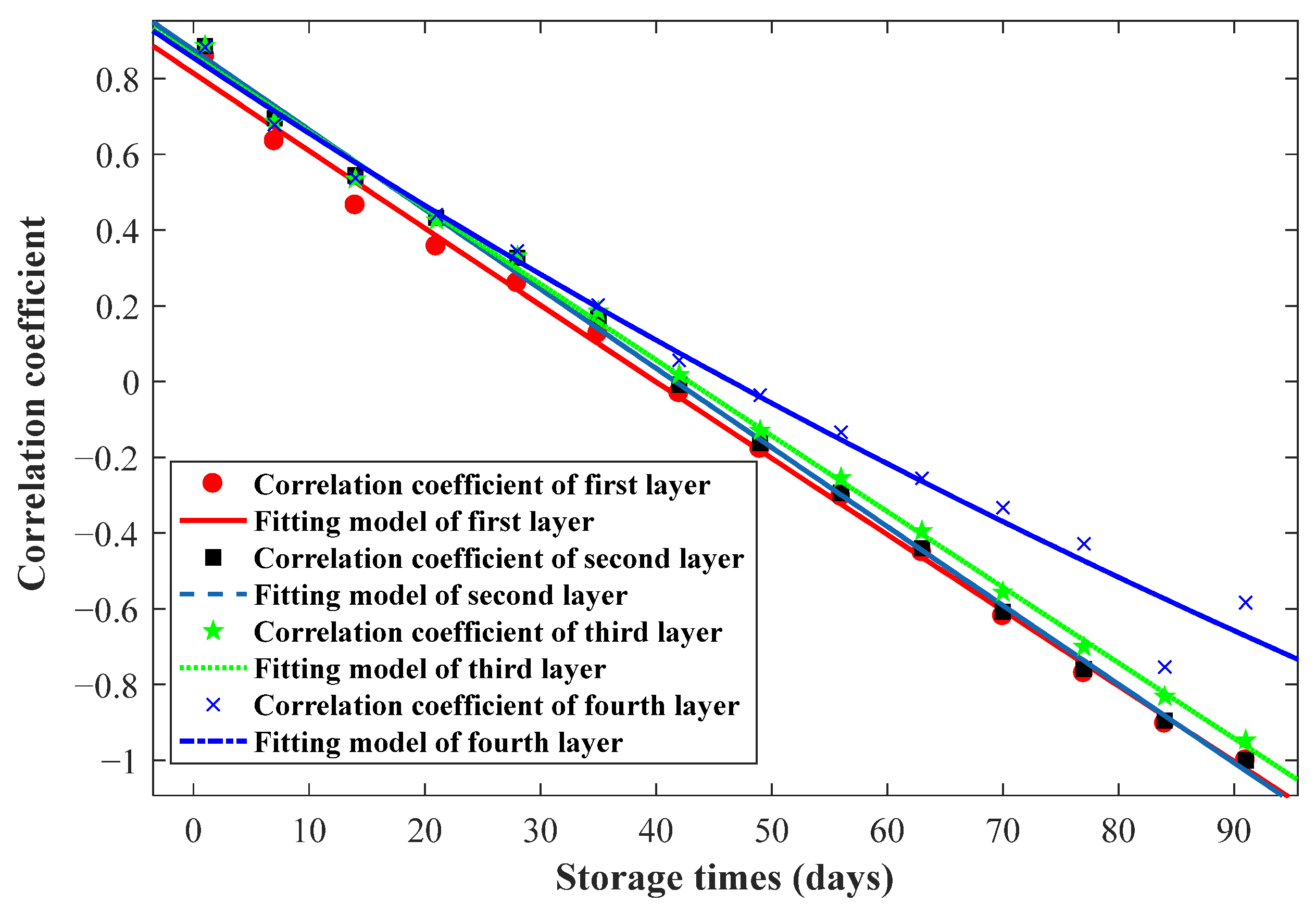
3.1.1. Models of Grain Temperature Correlation Coefficient Threshold on the XOY Plane

The correlation coefficient thresholds on the XOY plane were modeled with storage time as shown in Figure 4. The model parameters are shown in Table 2.
For the correlation coefficient thresholds of grain temperature on the XOY plane, the change trend of the model curves of the first to the third layers are basically the same, while the model curve of the fourth layer is quite different from them (Figure 4). Additionally, it can be seen that the correlation coefficient from the first to the third layers would be less than 0.8 when stored for about 10 days, and less than 0.6 when stored for about 20 days. In the short term (<49 days), the correlation coefficient of the fourth layer is basically the same as that from the first to the third layers. When the storage time is over 50 days, the correlation coefficient is slightly higher than that from the first to the third layers. The reason for this is that the fourth layer is close to the bottom of the grain bulk, and the grain temperature of the fourth layer is less affected by temperature changes in outside, and thus the grain temperature change is relatively insignificant and the correlation coefficient is high. Basically, the correlation coefficient thresholds of the first to the fourth layers set using the 3 σ -threshold method are the same, as can be observed in Figure 4b. The correlation coefficients decrease to the strong correlation interval (0.6~0.8) after about 5 days, and decrease to the weak (or no) correlation interval (<0.6) after about 10 days. The model parameters are shown in Table 2.

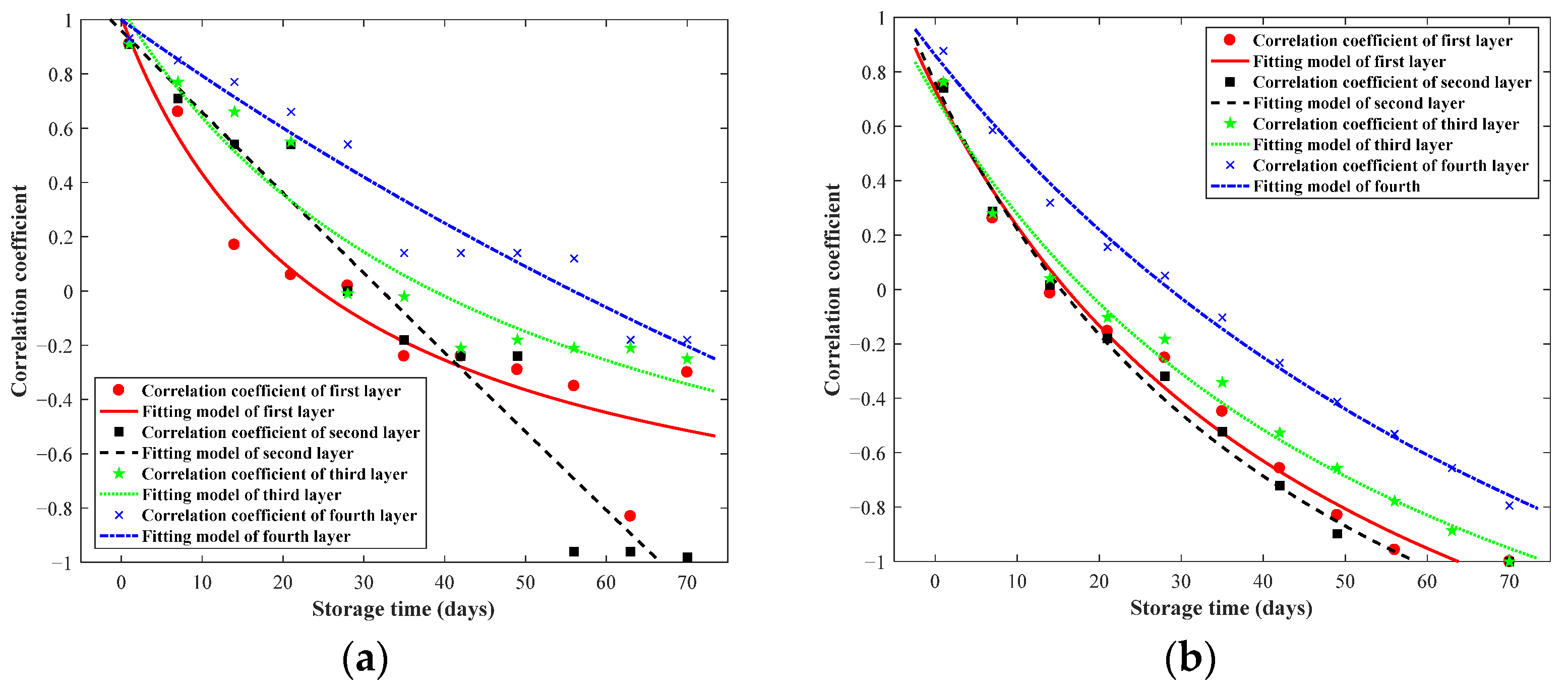
3.1.2. Models of Grain Temperature Correlation Coefficient Threshold on the XOZ Plane

The correlation coefficient threshold on the XOZ plane were modeled with storage time as shown in Figure 5, and the model parameters are shown in Table 3.
For the correlation coefficient thresholds of grain temperature on the XOZ plane, according to the fitting models based on the DBSCAN clustering results (Figure 5a), on the whole, the changing trend of the model curves of the second and fourth layers gradually slows down, and the model curves of the first and third layers are approximate to straight lines. The above conclusions can be verified from Table 3. Meanwhile, it can be seen that the correlation coefficient of each layer decreases to the strong correlation interval (0.6~0.8) when stored for about 5 days, and decreases to the weak (or no) correlation interval (<0.6) when stored for about 10 days. The model parameters can be seen in Table 3.
According to the fitting models based on the clustering results with 3 σ . (Figure 5b), the change trends of the model curves of the first, second and third layers are similar, and the model curve of the fourth layer is similar up until storage for 35 days, at which point the change trend becomes relatively flat. It can also be seen that the correlation coefficient of each layer decreases to the strong correlation interval (0.6~0.8) when stored for about 5 days, and to the weak (no) correlation interval (<0.6) when stored for about 10 days. The model parameters are shown in Table 3.

3.1.3. Models of Grain Temperature Correlation Coefficient Threshold on the YOZ Plane

The correlation coefficient thresholds on the YOZ plane were modeled with storage time as shown in Figure 6, and the model parameters are shown in Table 4.
According to the fitting models of the clustering results with DBSCAN (Figure 6a), the model curve of the first layer decreases most obviously up until storage for about 20 days, and then the rate of decrease gradually becomes slower. The model curves of the second and third layers have the same trend until storage for about 20 days. After that, the downward trend of the third layer slows down, while that of second layer maintains the same trend. The model curve of the fourth layer decreases more gently than those of the first to the third layers. Meanwhile, the points at which the correlation coefficient threshold of the different layers drops to each grade interval are different. For example, when the storage time is about 30 days, the correlation coefficient of the first layer is less than 0, the correlation coefficients of the second and third layers are between 0 and 0.2, and the correlation coefficient of the fourth layer is approximately equal to 0.4.
The models established according to the threshold set using the 3 σ -threshold method can be seen in Figure 6b. With increasing storage time, the model curves of the first to the third layers exhibit the same downward trend, and the downward trend of the model curve of the fourth layer is gentle. The reason for this is that the grain temperature changes in the fourth layer are more gentle than those near the outer side, and therefore, the correlation coefficient is higher. Meanwhile, it can be seen that the correlation coefficients of the first to the third layers are already in the strong correlation range (0.6~0.8) when stored for one day, dropping to the weak (no) correlation range (<0.6) when stored for about three days. When stored for about 10 days, the correlation coefficient is lower than 0.2. Meanwhile, when stored for about two days, the correlation coefficient drops to the strong correlation range (0.6~0.8) in the fourth layer, and the correlation drops to weak or no correlation (<0.6) when stored for seven days, reaching below 0.2 when stored for about 20 days.

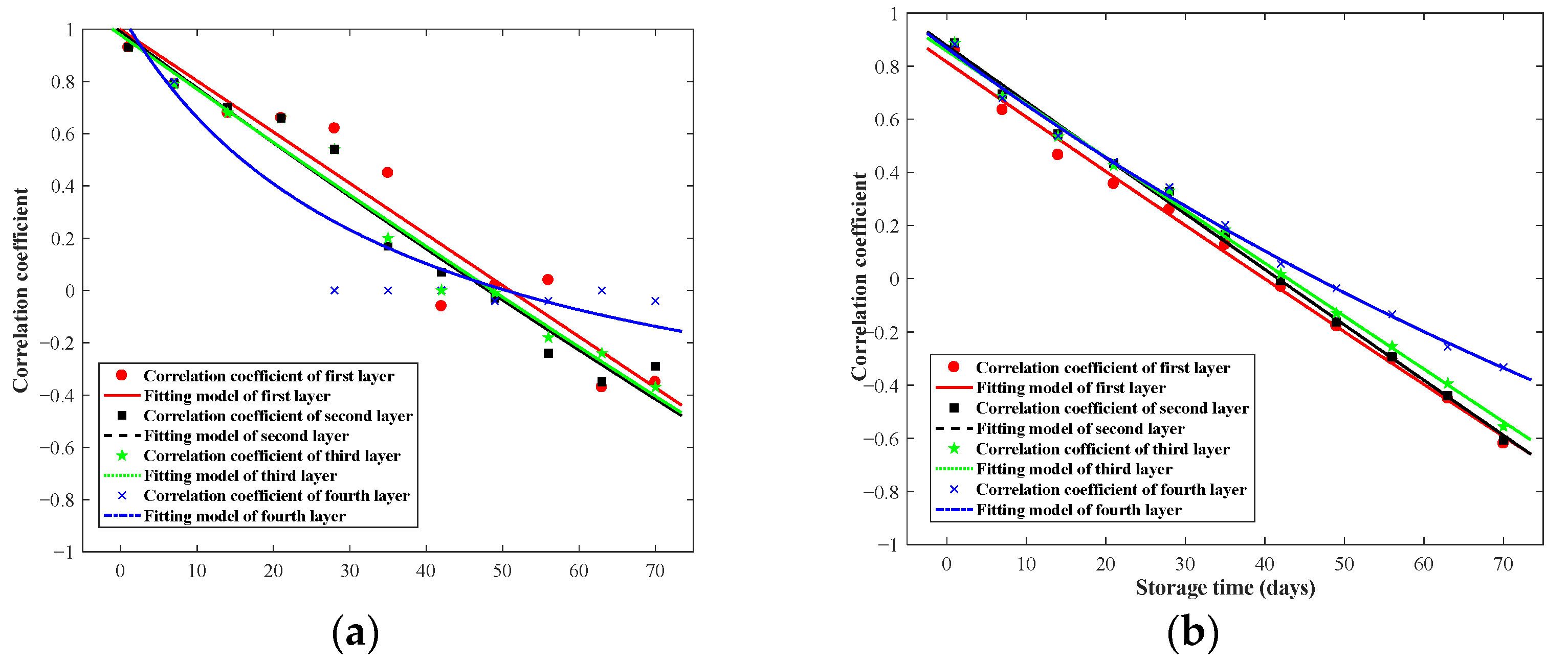
3.1.4. Evaluation of Threshold Setting Method

The indicators SSE, R2 and RMSE were used to the established models based on the clustering results, as shown in Table 5. The SSE of the established models based on the 3 σ -threshold method is lower than that of the established model based on the DBSCAN clustering results, indicating that the models based on the results of the 3 σ -threshold method possess a slightly better fitting effect. Comparing R2 and RMSE, the same conclusion can be reached. In general, the fitting effect of the model established based on the results of the 3 σ -threshold method is better than that of the model based on the DBSCAN clustering results.

3.2. Discussion

3.2.1. Influence of Empty Warehouse on Temperature Correlation

To verify the feasibility of the above threshold model in the detection of grain condition, the grain temperature data of a warehouse in Shaanxi Province during normal storage were selected, to analyze the influence of empty warehouse on the grain temperature correlation. The warehouse was unloaded around 10 April 2017 (a temperature field cloud map of the second layer on the XOY plane is shown in Figure 7), so the grain temperatures on 20 March 2017, 20 April 2017, and 20 May 2017 were selected to analyze the correlation coefficients of XOY planes, as shown in Table 6.
The correlation coefficients of grain temperature on 20 March 2017 followed by storage for 30 and 60 days are all less than 0.2 (Table 6). Compared to Figure 4b, it can be seen that the correlation coefficient of grain storage for 30 days is lower than the threshold, while the correlation coefficient of grain storage for about 60 days is higher than the threshold. This is because the correlation coefficients analyzed in Figure 4b come from multiple granaries. The grain temperature of some granaries changes greatly over 60 days, and the correlation coefficients are low. Meanwhile, the grain temperature of the other granary changes slowly, and correlation coefficients are high. Therefore, the empty warehouse destroys the grain temperature correlation on the XOY plane, but only for a certain period of time. In the same way, the empty warehouse (after unloading the warehouse) also destroys the correlation between grain temperature on the XOZ and YOZ planes.

3.2.2. Influence of New Grain on Temperature Correlation

The same granary in Section 2.2.1. was selected to analyze the impact of the addition of new grain on the grain temperature correlation. The grain was warehoused around 1 August 2017. Thus, the grain temperature data on 17 July 2017, 17 August 2017 (Temperature field cloud map of second layer in XOY planes in Figure 8) and 28 September 2017 were selected to analyze the correlation coefficient of the XOY plane, as shown in Table 7.
It can be seen from Table 7 that the correlation coefficient of grain temperature between 17 July 2017 and following its subsequent storage for about 30 and 60 days is less than 0.2, except for the fourth layer. Compared to Figure 4b, it can be seen that the correlation coefficient of storage for 30 days is lower than the threshold of normal storage for 30 days, while the storage for 60 days is higher than the threshold of normal storage for 60 days. The reason for this is that the grain was just loaded into the warehouse on 17 August 2017, and the temperature changed greatly, leading to a correlation coefficient with a value less than 0.2. In addition, after the warehouse was filled, the temperature changes of each point at that moment were basically the same as that when the warehouse was empty, resulting in the correlation coefficient between the two groups of temperatures meeting the threshold required normal storage for 60 days. Therefore, the new grain destroys the grain temperature correlation on the XOY plane, but only appears at a certain period of time. Similarly, the new grain also destroys the grain temperature correlation between the XOZ and YOZ planes.

3.2.3. Influence of Aeration Operation on Temperature Correlation

The same granary as that in Section 2.2.1. was selected in order to analyze the effect of aeration operation on the grain temperature correlation. The granary was ventilated on 10 October 2017 (a temperature field cloud map of the fourth layer on the XOY plane on 11 October 2017 is shown in Figure 9); thus, the grain temperatures on 21 September 2017, 20 October 2017 and 31 October 2017 were selected to analyze the grain temperature correlation of XOY planes. The correlation coefficients are shown in Table 8.
It can be seen from Table 8 that the grain temperature correlation coefficient on the second, third and fourth layers between storage on 17 September 2017 and about 30 days later is less than 0.2, which is inconsistent with the results presented in Figure 4b. In addition, the correlation coefficient between that and grain temperature after about 40 days of storage is about 0, which is basically the same as the correlation coefficient presented in Figure 4b. Therefore, aeration operation destroys the temperature correlation on the XOY plane, but only for a certain period. Similarly, aeration destroys the temperature correlation on both the XOZ and YOZ planes. Meanwhile, it can be seen that the grain temperature correlation coefficient of the first layer is greater than that from second to the fourth layers on 21 September and 20 October 2017. In addition, the grain temperature correlation coefficient of the first layer is much higher than them on 21 September and 31 October. The reason for this is that the grain temperature of the first layer is affected by the warehouse temperature and the grain temperature of first layer was lower than that of the second, third and fourth layers on 21 September. At that time, the cold air ventilated into the grain bulk did not significantly reduce the grain temperature of first layer. Therefore, a strong grain temperature correlation before and after the first layer was obtained for 40 days.

3.2.4. Influence of Self-Heating on Temperature Correlation

The grain temperature data of a granary in Heilongjiang in 2018 were selected to analyze the effect of aeration operation on grain temperature correlation. Since the granary experienced continuous self-heating from August to September 2018, the grain temperatures on 20 July 2018, 20 August 2018, and 20 September 2018 were chosen for subsequent analysis. A temperature field cloud map of the second layer on the XOY plane on 4 September 2018 is shown in Figure 10. The correlation coefficient of grain temperature on the XOY plane was analyzed, as shown in Table 9.
The correlation coefficients of grain temperature on the first and second layers between 20 July 2018 and after storage for about 30 and 60 days are all less than 0.2, which is inconsistent with the results shown in Figure 4b. The correlation coefficient of the third layer and the fourth layer are greater than 0.9, belonging to very strong correlation. The reason for this is the fact that the self-heating position in the granary is located between the first and second layers of the grain temperature measurement sensors, and the grain temperature of the third and fourth layers is not affected. Therefore, self-heating affects the grain temperature correlation on the XOY plane.
Ref. [21] used the correlation of grain temperature on the temperature measurement plane, line and point to perform the detection of abnormal changes in grain temperature in the grain bulk, and the threshold of the autocorrelation coefficient in the temperature measurement plane was set to 0.8, and the threshold of the change rate of the intercorrelation coefficient was (−0.15 d−1, 0.15 d−1). Ref. [34] presented a method in which grain temperature statistical parameters were used to detect grain inventory modes (empty and aeration) based on DBSCAN (density-based spatial clustering of applications with noise). The statistical parameters contained the grain temperature differences between adjacent layers, the aggregation ratios of four layers of grain temperature, the change rate of grain temperature, and the standard deviation of the change rate. The above research realized the detection of some grain storage states by using the statistical characteristics of grain temperature. However, they all ensure that there is a body of grain temperature data every day through the use of interpolation, and abnormal grain temperature is detected based on continuous grain temperature data. This study used the missing grain temperature data in the time domain for the purpose of statistical analysis, verifying that abnormal grain temperature states can also be detected by reasonably setting the threshold using missing grain temperature data in the time domain, making up for the deficiencies in the practical application of the above research.
In summary, up until 30 days of normal grain storage, the correlation coefficient of grain temperature on each plane is greater than or equal to 0.2. Empty warehouse, addition of new grain, aeration, and self-heating will cause the grain temperature correlation coefficient following storage for a certain duration to be lower than the correlation coefficient of normal storage. In particular, it will cause the grain temperature correlation coefficient value following for about 30 days to reach values less than 0.2, with a more obvious influence of self-heating on the grain temperature correlation at that location. Therefore, by rationally analyzing the correlation coefficient of grain temperature on each plane, it can be judged whether a grain storage state has occurred that caused a sudden change in grain temperature within a certain storage period (e.g., 30 days).

4. Conclusions

Two threshold setting methods for the grain temperature correlation coefficient on each plane under different storage durations were presented and used to analyze the variation law of the grain temperature correlation coefficient on each plane. The detection of abnormal changes in the grain conditions was verified on the basis of missing grain temperatures in the time domain. The main conclusions are as follows:
1. The lower limits of the correlation coefficient threshold interval for grain temperature set on the day and after storage for 1, 7, 14, 21, 28, 35, 42, 49, 56, 63 and 70 days on the XOY, XOZ and YOZ planes were obtained using the DBSCAN clustering method and the 3 σ -threshold method. Based on those thresholds, the models were established on the basis of the lower limit of the threshold interval and storage time. The models show that the correlation coefficient threshold decreases gradually with increasing storage time, and the correlation coefficient threshold is in the interval [−0.2, 0.2] when the storage time is about 30 days. The sum of squares of error (SSE), coefficient of determination (R2), and root mean square error (RMSE) were selected to evaluate the models. The indicators show that the model indicators established based on the threshold set using the 3 σ -threshold method were 0.056, 0.9771, and 0.0748, which is better than the values obtained for the model established using the threshold of the DBSCAN clustering method.
2. Grain condition states involving sudden changes in grain temperature (empty warehouse, new grain addition, aeration, and self-heating) will affect the correlation of grain temperature, and lead to the correlation coefficient being lower than the threshold during the normal storage. In particular, empty warehouse, new grain addition, aeration and self-heating cause the correlation coefficient of grain temperature to reach values lower than 0.2 following storage for about 30 days, which is the correlation coefficient threshold during the normal storage. Consequently, abnormal changes in grain conditions when there are missing grain temperature data in the time domain can be detected using the correlation coefficient threshold of grain temperature during normal storage in the time domain.

Author Contributions

Conceptualization, H.C. and Q.Z.; methodology, H.C. and W.W.; software, H.C.; validation, H.C., Q.Z. and H.Z.; formal analysis, H.C.; data curation, H.C.; writing—original draft preparation, H.C.; writing—review and editing, H.C., Q.Z. and H.Z.; visualization, H.C.; supervision, J.J. and H.M.; project administration, W.W. and H.M.; funding acquisition, H.M. All authors have read and agreed to the published version of the manuscript.

Funding

The present research was supported by Henan science and technology research program (No. 222102110215) and major science and technology project of Henan Province (No. 221100110800).

Institutional Review Board Statement

Not applicable.

Informed Consent Statement

Not Applicable.

Data Availability Statement

The data presented in this study are available on request.

Conflicts of Interest

The authors declare no conflict of interest.

References

  1. Wenhao, L. Research on Key Technologies of Internet of Things for Grain Monitoring and Control Based on Wireless Communication. Ph.D. Thesis, Henan University of Technology, Zhengzhou, China, 2017. [Google Scholar]
  2. Jingjing, B. Remote Monitoring and Early Warning of Fungus in Granary. Ph.D. Thesis, Henan University of Technology, Zhengzhou, China, 2019. [Google Scholar]
  3. Xiaomeng, W.; Wenfu, W.; Jun, Y.; ZhongJie, Z.; Zidan, W.; Qu, Y. Analysis of wheat bulk mould and temperature-humidity coupling based on temperature and humidity field cloud map. Trans. Chin. Soc. Agric. Eng. 2018, 34, 260–266. [Google Scholar]
  4. Xiaomeng, W.; Wenfu, W.; Jun, Y.; Zhongjie, Z.; Zidan, W.; Hongqing, Z. Research on temperature and humidity field change during corn bulk microbiological heating. Trans. Chin. Soc. Agric. Eng. 2019, 35, 268–273. [Google Scholar]
  5. Hongyang, G.; Xiaoping, H. Regional layout of China’s government grain reserves: Present situation, impact and optimization path. J. Huazhong Agric. Univ. 2021, 6, 27–34+187. [Google Scholar]
  6. Pingyuan, L.; Hong, J.; Qingfeng, F.; Weike, L. Discussion on the monitoring method of grain quality and safety and its effectiveness and timeliness. Grain Sci. Technol. Econ. 2017, 42, 18–20. [Google Scholar]
  7. Ling, L. Legislative proposals on improving the supervision & management mechanism of China grain reserves. J. Henan Univ. Technol. 2015, 11, 49–52. [Google Scholar]
  8. Xuecang, Z.; Pingfei, G.; Tong, Z.; Jianjun, W. Development and prospect of multifunctional grain condition measurement and control system. Grain Process. 2018, 43, 68–71. [Google Scholar]
  9. Panigrahi, S.S.; Singh, C.B.; Fielke, J.; Dariush, Z. Modeling of heat and mass transfer within the grain storage ecosystem using numerical methods: A review. Dry. Technol. 2019, 38, 1677–1697. [Google Scholar] [CrossRef]
  10. Quemada-Villagómez, L.I.; Molina-Herrera, F.I.; Carrera-Rodríguez, M.; Calderón-Ramírez, M.; Martínez-González, G.M.; Navarrete-Bolaños, J.L.; Jiménez-Islas, H. Numerical study to predict temperature and moisture profiles in unventilated grain silos at prolonged time periods. Int. J. Thermophys. 2020, 41, 52. [Google Scholar] [CrossRef]
  11. Novoa-Muñoz, F. Simulation of the temperature of barley during its storage in cylindrical silos. Math. Comput. Simul. 2018, 157, 1–14. [Google Scholar] [CrossRef]
  12. Qinqin, C.; Yang, L.; Xiaoliang, L.; Wangbao, W.; Hui, P.; Rong, J.; Qingye, S. Variation in paddy microbial communities under different storage temperatures and relative humidity. Food Res. Int. 2019, 126, 108581. [Google Scholar]
  13. Libing, J.; Yaqi, X.; Xinya, L.; Zhen, W. Numerical simulation and experimental study on temperature field of underground grain storage bin. J. Henan Univ. Technol. 2019, 40, 120–125. [Google Scholar]
  14. Mengmeng, G.; Guixiang, C.; Wenlei, L.; Chaosai, L. Simulation of Temperature Field of Paddy Grain Pile in Static Storage Based on COMSOL. J. Henan Univ. Technol. 2020, 41, 101–105. [Google Scholar]
  15. Chunyun, M. Study on the Numerical Simulation and Regularity of the Heat and Humidity Field of Corn Grain Piles without Artificial Intervention; Shenyang Normal University: Shenyang, China, 2017. [Google Scholar]
  16. Xiangxiang, Z.; Hao, Z.; Zhenqing, W.; Xi, C.; Yan, C. Study on temperature field of grain piles in underground grain silos lined with plastic. Trans. Chin. Soc. Agric. Eng. 2021, 37, 8–14, (Chinese with English Abstract). [Google Scholar]
  17. Mengmeng, G. Study on the Coupled Law of Heat and Moisture in the Ventilation Process of Bulk Wheat Grain Pile. Ph.D. Thesis, Henan University of Technology, Zhengzhou, China, 2021. [Google Scholar]
  18. Dexian, Z.; Miao, Z.; Qinghui, Z.; Yuan, Z. Granary storage quantity detection method based on bottom pressure estimation. Trans. Chin. Soc. Agric. Eng. 2017, 33, 287–294, (In Chinese with English Abstract). [Google Scholar]
  19. Zidan, W.; Qiang, Z.; Jun, Y.; Xiaomeng, W.; Zhongjie, Z.; Wenfu, W.; Fujun, L. Interactions of multiple biological fields in stored grain ecosystems. Sci. Rep. 2020, 10, 9302. [Google Scholar]
  20. Hongwei, C.; Wenfu, W.; Zidan, W.; Feng, H.; Jianpeng, D.; Yujia, W. Monitoring method of stored grain quantity based on temperature field cloud maps. Trans. Chin. Soc. Agric. Eng. 2019, 35, 296–298. [Google Scholar]
  21. Hongwei, C.; Wenfu, W.; Zidan, W.; Feng, H.; Haotian, Z.; Xiao, Q. Reserves monitoring method for grain storage based on temporal and spatial correlation of grain temperature. Trans. Chin. Soc. Agric. Mach. 2019, 50, 321–330. [Google Scholar]
  22. Xiao, Q. Research on the Strategies and Methods of Storing Grain Digital Supervision. Ph.D. Thesis, Jilin University, Changchun, China, 2018. [Google Scholar]
  23. Haotian, Z. Feature Extraction of Storage Grain Nephogram and Application of Supervision Method. Ph.D. Thesis, Jilin University, Changchun, China, 2019. [Google Scholar]
  24. Hongwei, C.; Wenfu, W.; Zidan, W.; Tianyi, L.; Jianpeng, D. Method to detect granary state based on statistical characteristics of grain temperature. Trans. Chin. Soc. Agric. Eng. 2020, 36, 320–330. [Google Scholar]
  25. Zhenfang, H.; Yuxia, Z.; Yang, C.; Dongfang, L.; Tong, Z.; Pengcheng, F.; Jianjun, W. Statistical character on temporal and spatial distributing of grain temperature in warehouse. Grain Storage 2010, 39, 15–20. [Google Scholar]
  26. Zhenqing, W.; Dongjie, T.; Haiyan, L. Experimental study on temperature field of underground reinforced concrete circular granary. J. Henan Univ. Technol. 2018, 39, 99–102, 126. [Google Scholar]
  27. Ruonan, L.; Yizhong, X.; Yan, L. Dynamic signature verification method based on Pearson correlation coefficient. J. Instrum. 2022, 43, 279–287. [Google Scholar]
  28. Akoglu, H. User’s guide to correlation coefficients. Turk. J. Emerg. Med. 2018, 18, 91–93. [Google Scholar] [CrossRef] [PubMed]
  29. Martin, E.; Hans-Peter, K.; Sander, J.; Xiaowei, X. A density-based algorithm for discovering clusters in large spatial databases with noise. In Proceedings of the Second International Conference on Knowledge Discovery and Data Mining (KDD-96), Portland, OR, USA, 2–4 August 1996; AAAI Press: Santa Clara, CA, USA; pp. 226–231. [Google Scholar]
  30. Weitun, W.; Yileh, W.; Chengyuan, T.; Mawkae, H. Adaptive density-based spatial clustering of applications with noise (DBSCAN) according to data. In Proceedings of the 2015 International Conference on Machine Learning and Cybernetics (ICMLC), Guangzhou, China, 12–15 July 2015; IEEE: Piscataway Township, NJ, USA; Volume 1, pp. 445–451. [Google Scholar]
  31. Xu, R.; Wunsch, D. Survey of clustering algorithms. IEEE Trans. Neural Netw. 2005, 16, 645–678. [Google Scholar] [CrossRef] [PubMed] [Green Version]
  32. Jianbin, H.; Jianmei, K.; Junjie, Q.; Heli, S. A hierarchical clustering method based on a dynamic synchronization model. Inf. Sci. 2013, 43, 599–610. [Google Scholar]
  33. Jing, L.; Jinqiu, H. A study of adaptive composite-indicator alarm threshold optimization of chemical process parameters. Pet. Sci. Bull. 2016, 1, 407–416. [Google Scholar]
  34. Hongwei, C.; Wenfu, W.; Zhongjie, Z.; Feng, H.; Zhe, L. Clustering and application of grain temperature statistical parameters based on the DBSCAN algorithm. J. Stored Prod. Res. 2021, 93, 101819. [Google Scholar]
Figure 1. Layout of temperature measurement sensors in the granary. The colored circles in the figure indicates the location of the temperature measurement sensors. The green, red and purple circles in the figure form three planes parallel to XOZ.
Agriculture 12 01883 g001
Figure 2. Layout of temperature measurement in the granary. (a) Plane parallel to XOY. (b) Plane parallel to XOZ. (c) Plane parallel to YOZ.
Agriculture 12 01883 g002
Figure 3. Model of the correlation coefficient threshold for grain temperature under different storage times.
Agriculture 12 01883 g003
Figure 4. The model of the grain temperature correlation coefficient threshold in the XOY planes: (a) fitting model of clustering results with DBSCAN; (b) fitting model of clustering results with 3σ.
Agriculture 12 01883 g004
Figure 5. The model of grain temperature correlation coefficient threshold on the XOZ plane. (a) Fitting models of clustering results with DBSCAN. (b) Fitting models of clustering results with 3 σ .
Agriculture 12 01883 g005
Figure 6. The model of grain temperature correlation coefficient threshold on the YOZ plane. (a) Fitting models of clustering results with DBSCAN. (b) Fitting models of clustering results with 3 σ .
Agriculture 12 01883 g006
Figure 7. Temperature field cloud map of the second layer on the XOY plane on 10 April 2017.
Agriculture 12 01883 g007
Figure 8. Temperature field cloud map of the second layer on the XOY plane on 17 August 2017.
Agriculture 12 01883 g008
Figure 9. Temperature field cloud map of the fourth layer on the XOY plane on 11 October 2017. The area with lower temperature in the middle is near the ventilated air duct.
Agriculture 12 01883 g009
Figure 10. Temperature field cloud map of the second layer on the XOY plane on 4 September 2018. The grain temperature in some areas of the middle exceeds 50 °C, which means that the grain is in the self-heating state.
Agriculture 12 01883 g010
Table 1. Relevance classification rule table.
RangesLevels
0.8~1.0Extremely strong correlation
0.6~0.8Strong correlation
<0.6Weak correlation or no correlation
Table 2. Model parameters of grain temperature correlation coefficient threshold on the XOY plane.
LayersDBSCAN
p1P2q1p1P2q1
First Layer−780.239,97039,860−44.6417842188
Second Layer−17.46840.4849.6−120.350125715
Third Layer−23.8911631190−309.113,26015,480
Fourth Layer−0.7437.2735.14−4.34201.9232.7
Note: DBSCAN is density-based spatial clustering of applications with noise. p1, p2 and q1 represent the coefficients of the model in equation 1.
Table 3. Model parameters of grain temperature correlation coefficient threshold on the XOZ plane.
PlanesDBSCAN3 σ
p1P2q1p1P2q1
First Layer−23.1512061247−984.339,15047,330
Second Layer−1.4469.9968.37−103842,47051,250
Third Layer−89342,71044,040−49.9819982362
Fourth Layer−1.85103.1106.9−5.81246.5287.5
Table 4. Model parameters of grain temperature correlation coefficient threshold on the YOZ plane.
PlanesDBSCAN3 σ
p1P2q1p1P2q1
First Layer−1.0926.5826.36−2.4639.2753.48
Second Layer−75.5224352538−2.5539.0851.47
Third Layer−1.2949.8547.75−2.4544.6663.06
Fourth Layer−5.22291.8292.2−3.2893.95109.1
Table 5. Evaluation of threshold setting results.
PlanesDBSCAN3 σ
SSER2RMSESSER2RMSE
XOY Planes0.12820.93230.12230.00800.99610.0314
XOZ Planes0.12090.93060.12220.11320.94960.1188
YOZ Planes0.17230.93320.14440.04670.98570.0742
Means0.14050.93200.12960.05600.97710.0748
Table 6. The influence of empty warehouse on the temperature correlation on the XOY plane.
XOY Planes20 March 2017 and 20 April 201720 March 2017 and 20 May 2017
First Layer0.133−0.184
Second Layer0.001−0.193
Third Layer−0.086−0.257
Fourth Layer−0.1130.322
Table 7. The influence of new grain on the temperature correlation on the XOY plane.
XOY Planes17 July 2017 and 17 August 201717 July 2017 and 28 September 2017
First Layer−0.2160.095
Second Layer−0.147−0.324
Third Layer−0.067−0.113
Fourth Layer0.3340.357
Table 8. The influence of aeration operation on the temperature correlation on the XOY plane.
XOY Planes21 September 2017 and 20 October 201721 September 2017 and 31 October 2017
First Layer0.1760.711
Second Layer−0.0070.068
Third Layer0.0480.067
Fourth Layer−0.0150.064
Table 9. The influence of self-heating on the temperature correlation on the XOY plane.
XOY Planes20 July 2018 and 20 August 201820 July 2018 and 20 September 2018
First Layer0.2340.574
Second Layer0.1490.186
Third Layer0.9740.911
Fourth Layer0.9750.946
Publisher’s Note: MDPI stays neutral with regard to jurisdictional claims in published maps and institutional affiliations.

