1. Introduction
According to the latest data presented by the International Grape and Wine Organization (OIV) in April 2020, the world viticultural area would be over 7.5 million hectares considering the area of grapes destined for winemaking, table grapes and raisins [
1]. In Chile, the total area of vineyards for winemaking currently occupies more than 192 thousand hectares, which have a potential for wine production close to 1200 million liters [
2]. Chile is currently the second-largest wine producer in America and the fourth world exporter of wines, being surpassed only by European countries with vast experience in winemaking matters, such as France, Spain and Italy [
3]. This is mainly found in the O’Higgins and Maule regions, concentrating more than 72% of the national area.
The collection of georeferenced spatial datasets, such as satellite imagery, allows winegrowers to optimize the decision-making process by showing the yield variability allowing them to take advantage of this variability for applying selective harvesting to increase the quality of the wine [
4]. Production of quality wines requires an adequate selection of fruit to be incorporated into the winemaking process [
5,
6]. Literature highlights the use of NDVI (Normalized Difference Vegetation Index) to manage a selective harvest and to relate quality factors, for example, sugar and acidity, to it. It has been verified that the NDVI value is linearly related to the leaf area [
7], fruit ripening, infestation and diseases, water status [
8], anthocyanin content of grapes [
9], tannins in the skin [
10], yield forecast [
6,
11] and maturity properties [
12].
In recent years, the availability of free data from satellites has generated a greater interest for its potential use in viticulture [
13,
14,
15], becoming an attractive solution for the spatio-temporal monitoring of many crops [
16], since it provides timely, synoptic, profitable and periodic information [
13], and it can be potentially used in operations of vine management, such as weeding and pruning [
17], enhancing the intra-parcel variability. This has been one of the focuses of precision viticulture, due to the fact that agricultural practices were traditionally applied in a uniform way [
18], with the same intensity or dose in operations such as pruning, fertilization, irrigation or phytosanitary treatments [
19]. According to Urretavizcaya et al. [
20], the variability has implications in the quality of the grape and in the profitability. Because of this, the identification, the spatial characterization, the interpretation of its oenological meaning, as well as the possibility of differential management of such variability, constitute the main objectives of Precision Viticulture [
21,
22].
Identifying intra-parcel variability has implications in the quality of wine, as well as the control in the maturation process [
18], essential information during the harvest, which depending on the type and size of the vineyard, is generally performed by combining manual and mechanized harvesting technology. The predefined plots are evaluated weekly after
veraison in order to measure the sugar and acid content, these are the most common parameters on which winegrowers rely to determine the correct time to harvest [
23]. Defining when and which plots will be harvested is based solely on the organoleptic evaluation carried out in the field daily. As Sun et al. [
24] graph, field observations of vine growth stages are too few to fully capture the spatial variability of vine conditions. Therefore, improving vineyard yield and grape quality through adequate knowledge of the spatial variability of the vineyard to reduce costs and environmental impact is one of the current challenges [
14,
22]. Optimizing the production of grapes for wine requires understanding the factors that influence its spatial and temporal variability, soil, climate, plant physiology and agricultural management which are responsible for different physiological expressions of the vine [
25]. Variability in vineyards is a problem widely studied in Australia, France, Spain [
26,
27], Chile [
28], New Zealand [
29] and Canada [
30], among others, confirming that this is a factor to consider to improve wine quality. The NDVI, one of the most used vegetation indices [
22], uses the visible (red) and near-infrared (NIR) spectral bands, which are closely related to the vegetative and productive characteristics of the crop [
14].
Wine quality is closely related to fruit quality, and the crop foliage is related to the interaction of soil, climate, water status and agronomic management, which are factors directly affecting fruit quality. Therefore, we can hypothesize that the use of spectral indices derived from Sentinel-2 images can provide indirect but valuable information about those variables directly measured in the fruit and that are indicators of wine quality, such as sugar and acidity. Furthermore, knowing their spatial distribution at key moments would contribute to better planning of differential harvesting for quality wine production. This study aims to contribute to the selective management of vine crops, through the use of satellite images of medium spatial resolution (Sentinel-2) from a two-fold perspective: (i) the analysis of spectral bands and indices to generate models that allow one to estimate °Brix (concentration of sugar in the berry) and pH; and (ii) to explore the use of Sentinel-2 imagery to differentiate and map the vine growing variability, in order to identify potential areas of early or late ripeness. This would imply a direct benefit to the selective harvest and, consequently, would presume a substantial improvement in the production and quality of wine.
2. Materials and Methods
This research includes the study of field data from two wine grape production harvest seasons: 2017 and 2018. Two batches (group of plots) of Cabernet Sauvignon variety, corresponding to adult plantations of the years 2007 and 2010, located in Viña Montes winery, commune of Santa Cruz, in the Colchagua Valley, VI region, Chile, were studied. Field data were periodically collected, allowing us to monitor the phenological state of the vine until the harvest. For this study, microvinifications were carried out in order to accurately evaluate the quality of the wine produced from the studied samples.
2.1. Study Area
Viña Montes is the company that owns the vineyards in which this study was carried out. It has a total of 720 hectares of vine and exports 93% of its production [
23,
31].
Figure 1 shows the specific study area. It is known as Arcángel and has a total planted area of 499 ha, with batches of different quality varieties such as Cabernet Sauvignon, Syrah and Carmenere, among others.
The area of interest in which this study is developed is made up of 23 plots. A plot corresponds to the polygon enclosing a group of rows of the same vine. In this case, they are grouped in two batches: 12 plots formed by 13 parcels that add up to a total of 64.8 ha and 11 plots formed by 12 parcels, totaling 71 ha, corresponding to plantations from years 2007 and 2010, respectively, as observed in
Figure 1. The batches are composed at 100% of the Cabernet Sauvignon variety, Alfa category, an intermediate quality category planted according to a 2 × 1 pattern. The harvest is carried out in a combined manner: manual in the plots historically known for having better quality and mechanized in those of lower quality. However, this differentiation is not strict and is decided during the ripening process.
The UTM coordinates WGS 84 Zone 19S, referring to the center of each batch are: Plantation 2007, E 254,096.003 m; N 6,197,606.610 m; Plantation 2010, E 255,503.426 m; N 6,195,483.135 m.
Cycle of the Vine and Meteorology of the Area
Most of the wine production in the world takes place in Mediterranean-type climates, characterized by high temperatures in the summer season, high light intensity and ambient humidity decreasing strongly throughout the day [
26]. Precisely, in the study area, a warm Mediterranean-type temperate climate predominates [
27], with a dry season of six months and a rainy winter with a total annual rainfall between 400 and 600 mm. In addition, the soils are of alluvial origin, with loamy-silty textures [
28].
The vegetative cycle of the vine begins when the grape buds start growing at the beginning of spring (September or October) and ends between April and May, generally.
The cycle may have some variations influenced by differences in growth conditions, temperature and rainfall [
29]. A significant increase in temperatures, added to a decrease in rainfall, would cause greater water stress in the plants. On the other hand, an increase in average temperatures and a reduction in thermal oscillation influences the aroma of the varietals and the color of the wines. Likewise, the increasingly dry autumns and occasional rains associated with intense events would imply greater irrigation requirements for the vineyards [
28].
In order to know the influence of rainfall on the phenological cycle of the vine, the cumulative rainfall during the previous year should be considered. In the case of temperatures, their influence is direct during the vine growing period. Therefore, in the case of the 2017 harvest, we should consider the cumulative rainfall from May to December 2016 and the temperatures of the season from January to April 2017. Likewise, for the 2018 harvest data, the rainfall of the previous year was reviewed, that is, May to December 2017, and the temperatures of the current cycle, from January to April 2018.
Figure 2 shows that the phenological cycle of 2017 is marked by the rainfall of the year 2016. This is scarce compared to the cumulative rainfall of the year 2017 (phenological cycle of the vine 2018), which doubled in relation to 2016 (
Figure 2). During the 2018 season, the air temperature was relatively lower than in 2017 during the vine ripening cycle. The temperature difference reached 1.99 °C, which is 11% lower. Solar radiation during the cycle was also slightly lower, reaching an average difference of −5.8%.
2.2. Data
2.2.1. Satellite Images
Figure 3 shows the acquisition date of a set of 16 images from the two years under study that were used in this work, the constellation Sentinel-2 is formed by two satellites in heliosynchronous orbit whose temporal resolution is 10 days per satellite or 5 altogether. Both satellites carry a multispectral image sensor (MSI) capable of acquiring images in 13 spectral bands, from 433 nm to 2280 nm. The red (665 nm) and near-infrared (842 nm) bands are of particular interest for agricultural applications since they allow the recovery of several vegetation indices at 10 m spatial resolution [
15].
The images used were acquired from the Sentinel-2A and Sentinel-2B platforms and downloaded at processing Level-1C, then atmospherically corrected to obtain surface reflectivities, using the Sen2cor application in the SNAP environment. The acquisition dates and level of processing of all the images used at different stages of the study are shown in
Figure 3. The Sentinel-2 images were downloaded directly from the Copernicus Open Access Hub platform (
https://scihub.copernicus.eu/dhus/#/home, accessed on 23 July 2021).
2.2.2. Field Data
The
veraison is a very important stage from the oenological point of view since, for the oenologist, the ripeness begins with this stage. Its duration is highly variable and can range from 20 to 50 days depending on the desired harvest point, the region and the variety. From this moment on, water, sugars and nitrogenous compounds are transported to the grain. The berries begin to increase in weight and size, but not by cell multiplication but by accumulation of nutritive substances (mainly sugars) and water, reaching their maximum size. At the end of this stage, the seed is able to germinate. It is also called physiological maturity [
30]. For this study, the samples were taken periodically at the same location, as shown in
Figure 4. Fruits were analyzed around two months before harvest. This analysis was carried out manually in the field, collecting samples of berries in order to know the state of maturity of the fruit and the probable alcoholic degree. The analyzed variables were °Brix and pH. The sugar concentration indicates the potential alcoholic degree of the wine to be obtained from the fruit. Thus, higher concentrations of sugar guarantee, under optimal vinification conditions, a higher alcoholic degree to quantify the sugar concentration. A refractometer with automatic temperature compensation, range 0–32% °Brix, was used. Within each sampling area, several berries were analyzed, and the average value was obtained for the corresponding sample point. pH is a measure of the concentration of free hydrogen ions and is a term used to determine acidity [
32]. Proper management of acidity is of fundamental importance, since it ultimately determines the quality of the wines [
33], and plays an important role in the sensory properties and balance of wines [
34]. The measurements were made with a pH meter.
2.3. Methods
2.3.1. °Brix and pH Data Sampling in the Field
The geographical location of the berry samples was based on the knowledge and identification of critical and homogeneous quality zones of historical wine production. This required the knowledge of the agronomist from Viña Montes. For the location of the samples, the historical NDVI of December and the Digital Elevation Model (DEM) of the area were used. Zones with common characteristics of vegetative expression and topography were defined and then the samples were spatially distributed homogeneously in the area of interest. From this categorization, the specific sampling positions were obtained for 15 points located in 14 plots (
Figure 4). Plot 7.08 had two sampling positions, which were averaged, with a total of 14 samples remaining throughout the area.
The central position of each sample was marked in the vineyard using GPS equipment. The data collection was carried out in a radius of 15 m from the central position, taking an average of 300 berries per sampling point. This procedure was used in both seasons. In the sampling process, only five berries were chosen per bunch: three berries from the shoulders of the bunch, one from the middle and one from the bottom.
2.3.2. Spectral Indices
Sentinel images were geometrically and radiometrically corrected and co-registered using ground control points. In the geometric correction process, the nearest neighbor resampling method was used, and the original pixel size was preserved. Eight of the thirteen Sentinel-2 bands were used, which correspond to: B3 (Green band—0.560 nm), B4 (Red band—0.665 nm), B5 (Red Edge band—0.705 nm), B6 (Red Edge band—0.740 nm), B7 (Red Edge band—0.783 nm), B8 (NIR band—0.842 nm), B11 (SWIR band 1—1610 nm), B12 (SWIR band 2—2190 nm), plus the generation of four spectral indices.
The reflectance in a 10-m pixel will be influenced by the foliage, the soil and, to a very low proportion, by the berries. Therefore, the main spectral variations are related to the variations in the foliage. For this purpose, four spectral indices calculated from the reflectance recorded in the different sensor bands were chosen. These indices are widely used in various agricultural applications: Green Normalized Difference Vegetation Index (GNDVI), Normalized Difference Vegetation Index (NDVI), Normalized Difference Moisture Index (NDMI), and Chlorophyll index.
NDVI ((NIR − Red)/(NIR + Red)) uses the Near-Infrared and the Red bands. NIR is known to show high reflectivity in healthy vegetation due to the leaves’ cell structure. Red stands out for its absorption or low reflectance due to leaf pigments, mainly chlorophyll. GNDVI ((NIR − Green)/(NIR + Green)) is a variant of NDVI but using the Green band instead of the Red one. In the case of the index called Chlorophyll ((Red − Blue)/Green), the visible bands are used, since this spectral range is dominated by the optical properties of the photosynthetic pigments of the leaves [
35]. The NDMI ((NIR − SWIR1)/(NIR + SWIR1)) uses the NIR and SWIR1 bands to determine the moisture content in the canopy [
36]. The SWIR1 band corresponds to the wavelength comparatively more similar to the Landsat shortwave band, base of this indicator [
37,
38,
39,
40].
The visualization of behavior and evolution of the vineyard allows one to overview the state of the plots and the development in both seasons. For this purpose, the NDVI was used, since this is considered an indicator related to the quantity, quality and state of vegetation [
41]. The best vegetative expression, or the maximum potential of NDVI, occurs in summer shortly before the
veraison, since just after this, the foliage begins to change, and near the harvest begins to lose leaves. The development cycle of the vineyard begins with pruning and new plantings in August/September; bloom in September/October; curdled in November/December;
veraison in January/February and finally harvest in March/April. Therefore, to characterize the entire development of each season, the NDVI image set runs from September to April.
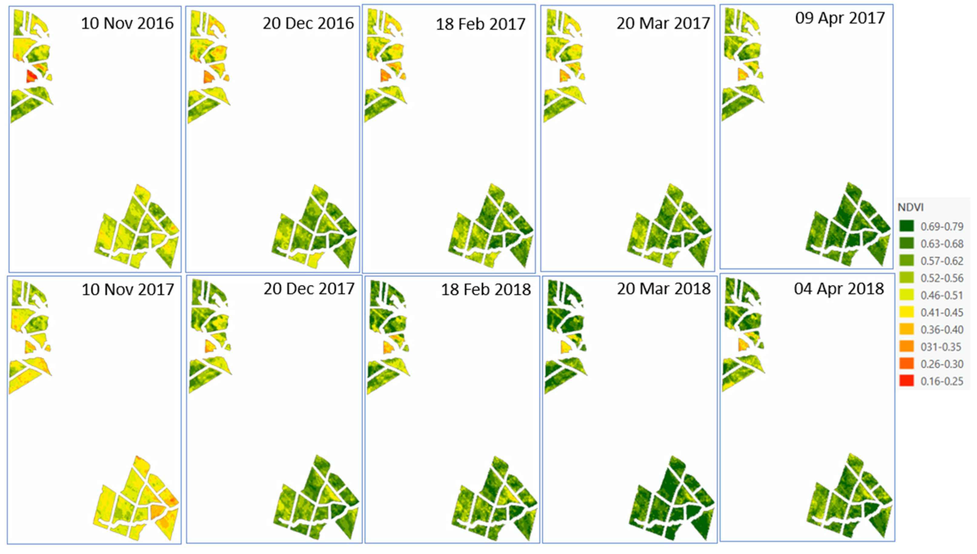
Figure 5 shows the NDVI maps displayed on a 10-rank scale. The plots are grouped by year of planting, 2007 and 2010. The 2007 plantation, located North, is made up of 12 plots and the 2010 plantation, located South, by 11 plots. In order to avoid mixed pixels in the boundary of the plots, a buffer of 15 m was applied to the limits towards the interior of the plots. For the characterization of the NDVI, eight image dates were used for each season. However,
Figure 5 shows only five of them per season.
Figure 6 shows the graphical comparison of the NDVI averages in the entire area, which shows how the 2018 season achieves better NDVI rates.
2.3.3. Modeling °Brix and pH
To determine the relationship between the °Brix and pH samples, and the bands and indices extracted from the Sentinel images, as well as the most explanatory variables, multiple linear regression models were used. An automated combination of the variables was carried out in order to select the best predictors and combinations. To determine the best regression and analyze the contribution of different variables to the model, a minimum of one and a maximum of five independent variables were used.
Table 1 and
Table 2 show the sampling data of °Brix and pH per date during the 2017 and 2018 seasons, allowing for a general view of the evolution of the samples in the vineyard. The dates in
Table 1 and
Table 2 correspond to the field data acquisition date. The plot samples were acquired in an average of plus or minus one day with respect to the date indicated in the Tables.
Figure 7 shows the comparison between both seasons Brix (a) and pH (b).
The average of pixels located in a buffer of 15 m around the sampling point was considered to be representative of the variables measured in the field. For each sampling date, a table was created to show, in each plot, the value of the sample corresponding to the average of the berries taken around a radius of 15 m, and the average of pixels obtained from the images as indicated in
Table 3. In summary, 14 samples with 12 independent variables per date were used to determine if there was a combination of variables that explained the sugar content and the pH values in the berries.
3. Results
3.1. Comparison of Coefficient of Determination R2
The determination of the °Brix and pH models begins with the selection of the best regression model from the combination of multiple variables. The regression model was obtained considering the best predicted variable in each date. From the image, all pixels within a 15-m radius circle around the terrain sample were considered. By the adjustment of ordinary least squares, the information on the multiple regression models was obtained, from which the statistical values of validation of each model and the equation of the adjusted model for each case were derived. According to the results in °Brix, the comparison of the R
2 in both seasons shows that, in general (
Figure 8), the 2017 season reaches better coefficients from mid-March with two variables; unlike the 2018 season that occurs at the end of March. In the case of the 2017 season, with three variables onwards, regardless of the date, the coefficient of determination does not fall below 67%.
Table 4 shows the results of the models with a higher correlation, considering a maximum of three variables, with respect to the samples acquired on 19 March 2017, with 14 samples and 1585 adjusted models.
Table 4 shows several statistical indicators: CME corresponds to an estimate of the variance of the deviations with respect to the adjusted model; R
2 is the percentage of variation in the response that is explained by the model; Adjusted R
2 is the percentage of variation in the response that is explained by the model, adjusted based on the number of predictors in the model relative to the number of observations, and it is used to compare models that have different numbers of predictors; Mallows Cp compares the precision and bias of the full model with those models that have the best subsets of predictors. A small Cp indicates that the model is relatively accurate (has a small variance) in estimating the true regression coefficients and forecasting future answers.
As shown in
Table 4 referring to °Brix and pH, this method allows one to visualize which models give the highest values of R
2. The adjusted R
2 statistic measures the proportion of variability in °Brix (values on the left of the Table) or pH (values on the right of the Table) that is explained by the model.
Regarding
Table 5, which summarizes the results for °Brix, the °Brix determination coefficients are very stable in 2018, with the best R
2 presented at the end of March. In the case of the 2017 season, the results are very homogeneous and with high coefficients, over 60% by the end of March and the beginning of April.
When focusing on the pH results, the comparison of R
2 in both seasons shows greater stability in the dates since the highest R
2s are concentrated in the sampling of 19 March (
Table 6). For the 2018 season, the highest R
2s are split between 13 March and the end of March.
Unlike the °Brix modeling, the case of pH in all combinations reaches lower values, although it improves discretely during the 2018 season, as can be seen in
Table 6, which considers the average of all sampling dates in relation to the number of variables for both °Brix and pH.
Regarding the variables used to model sugar accumulation, the repetition of a model based on the two short-wave infrared bands and the NDVI (GHL) stands out in particular. This combination is repeated in both seasons, in 2017 with an R2 of 67.64 and in 2018 of 53.48.
In the case of pH, the coefficients of determination are very stable in 2017, with the best R2 being in the middle of March. In the case of the 2018 season, the results are less homogeneous; coefficients greater than 60% have been observed since mid-March.
The repetition of combinations of variables in the pH modeling occurs more frequently than in the °Brix model. In the case of two variables, it is repeated (B11, NDVI) with an R2 of 17.6% in 2017 and of 50.1% in 2018. Then, in the combinations with four and five variables, the same variables are repeated. In the case of four variables, (B3, B4, Chlorophyll and GNDVI) are presented with R2 of 68.8% in 2017 and 79.1% in 2018 and, finally, (B3, B4, B5, Chlorophyll and GNDVI) with R2 of 89.8% in 2017 and 85.3% in 2018.
The statistics obtained in the °Brix and pH modeling are observed in
Figure 9 and
Figure 10, including the scatter plot for the values of the sampling points in relation to the observed values regarding the predicted ones.
To summarize the behavior of both seasons, the 2018 season achieved better quality indices referring to the accumulation of sugar and acidity. This season had greater accumulation of total rainfall, it was cooler in terms of seasonal temperature, it reached earlier rates of vegetative vigor, it reached a better average of NDVI in both the 2007 and 2010 plantations and, consequently, reached a level of °Brix and pH slightly better.
3.2. Applied Model
Table 7 shows the equations of the selected models for °Brix and pH, using a maximum of three variables, in both seasons.
Since these models are different depending on the date, their precision is limited in time, which implies that they should be obtained monthly. This time limitation does not restrict the benefits of this tool in the objective of this study, since they allow the zoning where the next sampling will be carried out, thus allowing one to improve the precision to determine the maturity and optimize the harvest moment of each plot.
3.3. °Brix and pH Maps
By applying the models with three variables for years 2017 and 2018, representative maps of the state of °Brix and pH on a particular date can be obtained, showing the variability of each plot concerning the ripening potential. This allows us, by using a limited number of field samples and Sentinel-2 images, to estimate those variables for the entire plot. Although the generation of these maps does not preserve from the collection of field data, it makes the field quality sampling process more efficient, as it facilitates the identification of ripeness variability and, subsequently, zoning and determining where to perform the field sampling.
Figure 11 and
Figure 12 compare the NDVI map with the °Brix map obtained by applying the models for the years 2017 and 2018, respectively. In general, the modeling enhances with higher °Brix values the areas with low vegetation index. In the image corresponding to °Brix, both in the 2017 and 2018 seasons, the intra-parcel variation is notorious, in a similar way as in the NDVI image.
In the case of the pH maps (
Figure 13 and
Figure 14), even if variability exists, there is no correspondence, as in the case of NDVI and °Brix. Unlike what occurs with °Brix and NDVI, there are no obvious relationships between vigor and pH, nor high intra-parcel variation of pH.
4. Discussion
In our work zone, we found that the NDVI had different behavior when comparing both seasons. The general average of NDVI was lower in the 2017 season compared to the 2018 season, the year in which the cumulative rainfall was doubled. These results allow us to relate the cumulative rainfall to the early vigor of the second season. Indeed, as stated by Hall et al. [
42], the soil-related effects in a given field will vary from season to season and can be completely reversed in different rainfall conditions. Although the meteorological variables were addressed in this study as a precedent for the area and not as a variable, there were temperature differences of up to 4° in the first half of January, and cumulative precipitation was doubled compared to the previous one in the 2018 season. Trought et al. [
43] suggested that small differences in temperature may have an influence on the phenology of the vine. In our case, the average °Brix increased slightly during 2018, a cooler year and with less radiation than its predecessor in the summer months prior to harvest. Although it is expected that higher temperature and radiation facilitate the accumulation of sugar, authors such as Abeysinghe et al. [
44], in Australia, found that berry growth was delayed by the heavy shade of the grape leaves, but the rate of sugar accumulation was not affected. If we take into account these studies, and that the best models occur at dates closer to harvest, it would be desirable to consider the climatic conditions as an additional variable that could improve the estimated model.
Other studies have determined the importance of climatic conditioning factors in anthocyanins. It must be said that with the onset of
veraison, sugars and anthocyanins begin to accumulate together, being both in a direct relationship [
45]. However, as a result of temperature changes, a gap between sugars and anthocyanins could be caused, as well as the alteration of their accumulation and degradation pathways [
46]. These studies give strength to determine that conditions such as luminosity and temperature are the main environmental variables that regulate the formation of anthocyanins. Del Valle et al. [
47] state that luminosity stimulates it and high temperatures inhibit it. Likewise, Peña [
48] states that the climate of the area and its thermal and light effect have a great influence on the entire development process, affecting photosynthesis and the formation of sugars and acids. In the same way, Gutiérrez-Gamboa and Moreno-Simunovic [
49] indicate that the climatic conditions affect the ripening of the grape more than the characteristics of the soil. The influence of cumulative rainfall on the ripening process is therefore questionable, which would be interesting to address in future works and compare with other seasons. Satellite images gain real importance as they have the ability to record the spatial variability of the vineyard, very fundamental knowledge in order to make decisions about the agronomic management of vineyards [
50]. Currently, electronic sensors are used to detect variability between plots in order to allow the application of differentiated management in specific sites for the most important field operations, such as fertilization, pruning or harvesting [
51]. Indeed, as Arnó et al. [
52] said, there is little doubt that selective harvesting can provide economic advantages for more sustainable and competitive viticulture. In this sense, the results of this work show the possibility of mapping the spatial variability of quality indicators of wine grapes, such as °Brix and pH, not only between plots but also within plots, by obtaining models derived from spectral indices derived from Sentinel-2 images. Although these models do not achieve sufficient reliability to obtain precise estimates of these indicators at the plant level, they are very useful for the differentiated management of harvests, providing spatial information for selective harvesting in order to categorize different types of wine.
5. Conclusions
Determining a model that allows one to define a differentiated harvest, according to the variability of the plot and therefore the possible areas of early or late ripeness of the vineyard, is very useful to obtain an improvement in production and therefore in the quality of the wine. The purpose of this research was to determine these variations by modeling, from variables extracted from Sentinel-2 images, two of the fundamental factors of wine quality: the accumulation of sugar, measured in degrees °Brix, and the pH. The work was carried out in two harvest seasons and four dates prior to harvest were considered. In both seasons, the °Brix models obtained determination coefficients higher than 60% from mid-March onwards. In the case of pH, although the relationship tends to be lower than in the case of °Brix, there is a relationship that can be used as an indicator of the intra-parcel variability to improve in practice agronomic management. A coefficient of determination of 43% and 63% for the pH prediction models in the 2017 and 2018 seasons, respectively, indicates the need to improve the study in the future, by increasing the number of samples.
The maps generated from the built models can be used as a tool to show the spatial variability of the sugar content and its acidity in the entire area. This tool may allow, semi-automatically and with high reliability, the division of the cultivation plots into several regions with homogeneous characteristics (°Brix and pH) that could receive differential treatment at harvest. The objective of optimizing all the processes in the wine production chain is to raise the quality level of winemaking, favoring optimal management of all phases. Incorporating technological solutions, such as the use of satellite images to the fruit sampling process, allows improving an artisanal process, by generating a map of predicted values of °Brix and pH. This permits defining the key areas to review in the field, increasing the possibilities of carrying out a directed harvest, through site-specific sampling, which gives the ability to take decisions in vineyard management. At this point, free satellite images with high periodicity are accessible even for smaller vineyards, giving the possibility to determine areas within the plots that should be studied and eventually harvested in a differentiated way, since an adequate selection of grapes with similar characteristics is a key factor to improve the quality and productivity of winemaking.


