Poplar-Assisted Bioremediation for Recovering a PCB and Heavy-Metal-Contaminated Area

Abstract

A Monviso clone has been applied to promote PCB degradation in a soil historically contaminated by polychlorinated biphenyls (PCBs) and heavy metals (HMs). The multi-contaminated area is located in Southern Italy. PCBs, HMs, and the soil microbial community (abundance, viability, and structure) were analysed in selected plots of the poplar-treated area. At 900 days after poplar planting, chemical analyses showed that PCBs and most of HMs diminished under the Italian legal limits. The overall results suggest that the poplar clone was effective in promoting PCB rhizodegradation and HM phytostabilization. Organic carbon content increased strongly in the rhizosphere of the planted plots. Microbiological results highlighted an overall increase in microbial abundance, cell viability, and the presence of bacterial groups involved in PCB degradation. The poplar-based bioremediation technology is a nature-based solution able to promote the recovery of soil quality in terms of contaminant removal, increase in organic carbon, and stimulation of autochthonous bacterial groups able to transform PCBs.

1. Introduction

Natural ecosystems have profoundly been affected by harmful waste materials and xenobiotics coming from various anthropogenic sources, resulting in a threat to biota and human health [1]. Among them, heavy metals and organic pollutants are of particular concern for their persistence and hazardous effects [2], depending on their intrinsic chemical properties, which favour their toxicity [3]. Heavy metals naturally exist in the earth’s crust, but some of them, such as cadmium (Cd), chromium (Cr), copper (Cu), mercury (Hg), lead (Pb), nickel (Ni), zinc (Zn), and arsenic (As), are widely used in industries and agriculture, and consequently, they are continuously found in the environment [4].

Soil is the final receptor of most hydrophobic organic contaminants, such as PCBs, which can also come from other environmental matrices. PCBs are synthetic organic compounds obtained from the chlorination of a biphenyl molecule; they are classified into 209 different congeners, according to the number and position of the chlorine substitutes. These molecules are highly soluble in nonpolar solvents, and the higher the number of chlorine atoms, the lower their water solubility and vapour pressure [5]. Due to their being bound to organic matter, PCBs can be rapidly adsorbed on the soil particle surface. In this regard, a recent study showed that the sorption of PCB congeners onto the soil is highly dependent on the amount of soil organic matter and on the surface area and pore size distribution of the soil particles [6].

Environmental restoration is required when the concentration of these pollutants is above defined legal limits [4]. For this purpose, plant-based remediation technologies are gaining popularity as they are a sustainable and cost-effective solution for soil clean-up from chemical contamination.

Many plant species are able to accumulate toxic metals into their vegetative and reproductive parts. This process is particularly influenced by the type of plant species and by the distribution of metals in the different fractions of the soil. The root system, through the production of some molecules, such as sugars, phytosiderophores, and organic acids, can favour the extraction of metals from the soil solution, mobilizing them towards the root surface. Here, some metal ions can pass through the selectively permeable cell membrane and can be then transported to the aerial parts of the plant. Rhizosphere microbial communities can support plant growth, making them much tolerant to high metal concentration, and they can also increase the success ratio of phytoremediation processes by recycling nutrients, maintaining soil structure, controlling disease, and reducing metal toxicity level [7].

The complex interactions occurring between the root system of a selected plant species and the soil autochthonous bacterial communities in the rhizosphere can significantly increase the biodegradation of recalcitrant organic pollutants [8].

The pathway of biodegradation of chlorinated organic compounds has been identified. It proceeds through various steps and involves different microorganisms. The entire mechanism is based on two major microbial metabolic steps: (i) anaerobic reductive dechlorination of higher-chlorinated congeners and (ii) aerobic degradation and cleavage of the biphenyl structure. Sequential anaerobic–aerobic transformations are required for complete PCB mineralization [9].

Plants play a crucial role in PCB degradation by exuding amphiphilic molecules, which increase PCB bioavailability. These molecules are surfactants that can enhance the bioaccessibility of some PCB congeners to biodegradation by microbial consortia [10].

In the last years, several microcosm studies have been carried out to evaluate plant species capacity in recovering PCB-contaminated soils [11,12,13]. Field-scale applications are still at a small number.

The present study aims at assessing the effectiveness of a poplar-based bioremediation technology applied at a historically PCB- and heavy-metal-polluted soil for two and a half years (900 days). A selected Populus clone (Monviso), previously applied to successfully remediate a contaminated soil from hexachlorocyclohexane [14], was planted in a multicontaminated site located close the city of Taranto (Italy) [15]. Before starting the plant-assisted bioremediation, chemical investigations of the area highlighted a diffuse contamination by PCBs and HMs. In this work, these contaminants and the soil microbial community (abundance, viability, and structure) were analysed in selected poplar-planted plots and in unplanted soil (controls) outside the poplar cultivation. The main processes involved in the PCB and HM plant-assisted bioremediation, including the role of soil microbial communities in the overall processes, are reported and discussed.

2. Materials and Methods

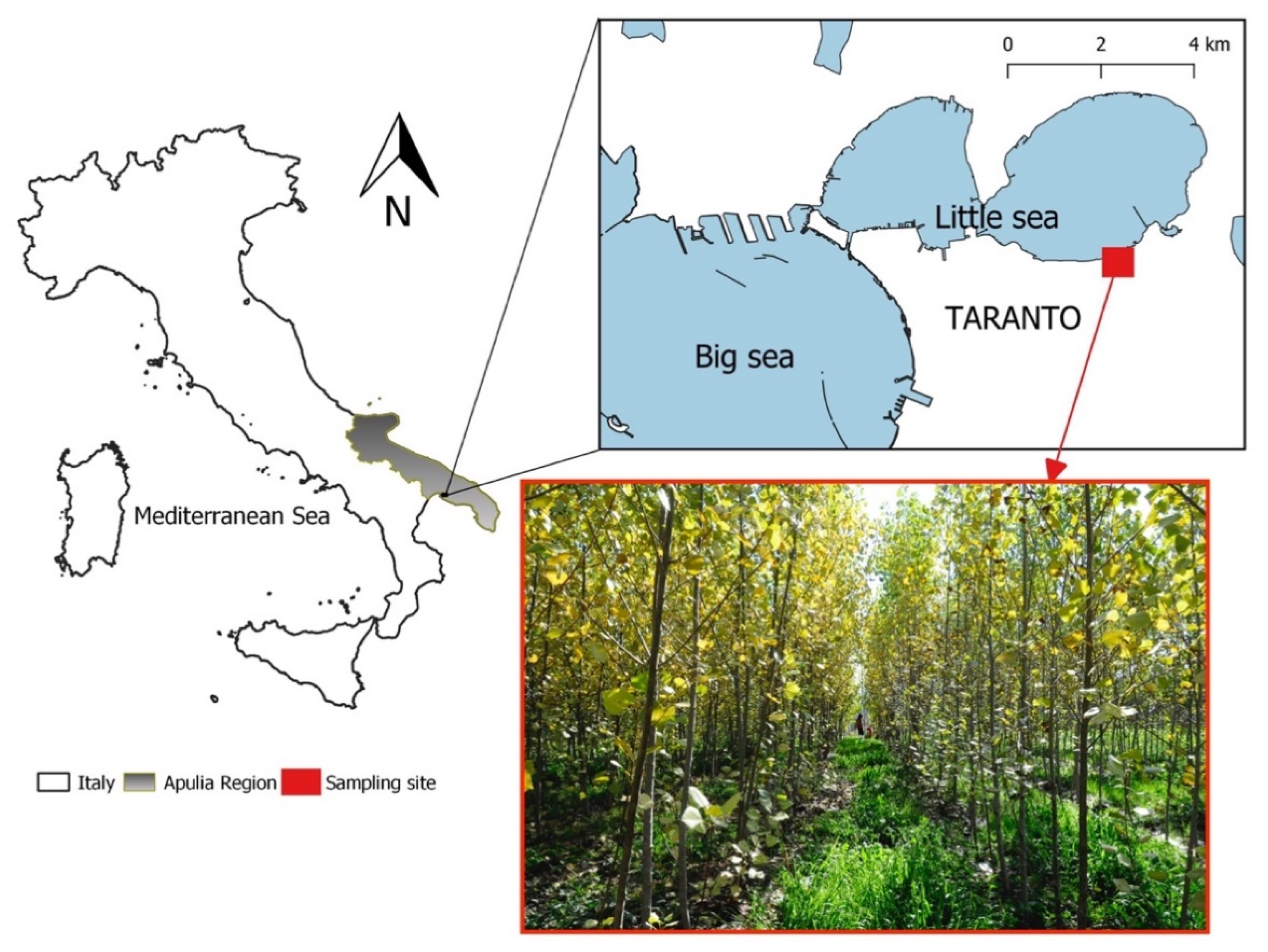
2.1. Site Description

The study site is a degraded area of ≈4.5 Ha located in the Apulia Region near the city of Taranto (40°28′04.92″ N, 17°18′12.68″ E) (Figure 1). The city of Taranto (Italy), during the 1960s, was subjected to an intense industrialization process with the construction of a large industrial district close to the urban areas that completely changed the natural environment [16]. Numerous anthropogenic activities influenced the biogeochemical characteristics of waters, sediments, and soils, making the area severely polluted by heavy metals and organic contaminants [17,18]. The main environmental impact that affected the specific study site was a small power station with transformers, and uncontrolled spilling and improper disposal of dielectric fluids resulted in polychlorinated biphenyl (PCB) pollution over a period of 30 years. Moreover, since the same site was used as an abusive waste dump, different waste layers (e.g., construction rubbish, polluted sediments originating from the “Mar Piccolo” facing it) also accumulated above the original limestone soil.

2.2. Experimental Design

In April 2013, a poplar-assisted bioremediation technology was applied for restoring the survey area contaminated by PCBs and HMs. A total of 650 cuttings of the Monviso clone were planted in a 785 m² subarea of the previously chemically characterized site [15].

In April 2013, about 650 poplar cuttings were planted in 8 rows 2 m apart in a subarea of the survey area measuring 785 m². Inside each row, the cuttings were arranged at a distance of 0.5 m from each other. A first sampling campaign carried out at 14 months from poplar planting evidenced a general decrease in PCBs and HMs thanks to the poplar-assisted bioremediation strategy adopted.

In this work, we report the results of a further sampling carried out at 30 months (900 days) after planting. As in the previous sampling, two contaminated plots were sampled. They were selected for the highest initial values of PCB contamination (i.e., average values of about 240 ng/g), which exceeded the Italian legislative limit (Italian Decree 152/06) of 60 ng/g for green areas [15].

The area of each plot was 1 m²; a target tree was identified at its centre. Inside each plot, sixteen sub-samples of soil, at different distance and depth from the tree trunk, were collected and used to create four composite soil samples labelled as follows:

• − A: 0.25 m distance from the trunk and 0–20 cm depth;
• − B: 0.25 m distance from the trunk and 20–40 cm depth;
• − C: 1 m distance from the trunk and 0–20 cm depth:
• − D: 1 m distance from the trunk and 20–40 cm depth

For each plot, a rhizosphere soil sample (Rizo), surrounding the root system of the target tree, was also collected.

The composite sampling strategy adopted, has been reported in detail in Ancona et al. [15].

Moreover, a 1 m² untreated contaminated point (outside the poplar-planted area and without any plant species) was identified as control.

This work reports the results of two selected multi-contaminated plots (P1 and P1bis), obtained at 900 days after poplar cuttings plantation. In particular, soil samples collected at the different distances and depths from each target plant (Rizo, A, B, C and D) and, plant tissues (leaves, shoots and roots), were processed for physical-chemical and microbiological analyses.

2.3. Chemical Analyses

2.3.1. Soil Properties

Physical–chemical analyses were performed to evaluate soil quality and possible nutritional deficiencies that might affect plant growth. Sample preparation was performed following Ancona et al. [15]. About 500 g of each soil sample was analysed for pH (H₂O), water content, organic C content, and available P using standard methodologies for soil chemical analyses [15].

2.3.2. PCB Analyses

Soils and plant tissues were air-dried for 2 days and then pulverized in a ball miller equipped with zirconium oxide jars (Retsch MM301 Mixer Mill, Haan, Germany) and homogenised prior to the PCB extraction.

PCBs were extracted from 1 g of each soil sample and 5 g of each plant tissue (leaves, shoots, and roots) using an accelerated solvent extractor (ASE 300 Dionex, Sunnyvale, CA, USA), as reported in detail in Ancona et al. [15]. A known amount of two labelled PCB standards (¹³C-PCB194 and ¹³C-PCB104) was added to each sample prior to extraction for monitoring the procedure efficiency. An OPR (ongoing performance recovery), consisting of a blank sample spiked with both labelled and native PCB standards, was also extracted in order to check the GC–MS performance recovery during the analysis.

All the extracts were evaporated under a gentle nitrogen stream and concentrated up to 0.5 mL in n-nonane using a TurboVap concentration workstation (TurboVap II, Caliper Life Sciences) [15]. All samples were analysed with a GC system (7980B GC, Agilent Technologies, Santa Clara, CA, USA) coupled to a Triple Quad/MS System, 7000c GCTQ (Agilent Technologies, Santa Clara, CA, USA) equipped with an electron impact (EI) ion source. The column used for the separation was an Agilent 122-5562 UI DB 5 ms Ultra Inert (60 m × 250 µm × 0.25 µm) operating at a flow rate of 1.2 mL/min with helium (He) as a carrier gas with a flow rate of 2.25 mL/min and N₂ as a collision gas with a flow rate of 1.5 mL/min. A multistep gradient with the following parameters was applied: the oven temperature was held at 80 °C for 1 min, increased first to 185 °C at a rate of 25 °C/min and held for 1 min, then increased to 210 °C at a rate of 5 °C/min and held for 10 min, further increased to 280 °C at a rate of 5 °C/min, and finally increased to 310 °C at a rate of 30 °C/min held for 10 min. Helium (He) was employed as the carrier gas with a flow rate of 2.25 mL/min, and nitrogen (N₂) was the collision gas with a flow rate of 1.5 mL/min. A volume of 1.0 µL of each sample was injected. A total of 19 PCB congeners were detected and quantified according to their mass transitions: 12 Dx-L (dioxin-like) congeners (PCB77, PCB81, PCB123, PCB118, PCB114, PCB105, PCB126, PCB167, PCB156, PCB157, PCB169, and PCB189), 6 marker congeners (PCB28, PCB52, PCB101, PCB153, PCB138, and PCB180), and 1 non-Dx-L congener (PCB128). A 5-point calibration curve, in which each standard solution contained a known amount of each native congener and the labelled internal standard (¹³C-PCB104), was used for the quantification. The final concentration was expressed as ng PCBs/g of dry sample. Average values of at least 2 replicates were taken for each analysis. The limit of detection (LOD) and limit of quantification (LOQ) of the procedure were determined to be 0.063 ng/g for each PCB congener.

2.3.3. HM Analyses

Trace elements (Be, Al, V, Cr, Fe, Co, Ni, Cu, Zn, As, Se, Cd, Sn, Sb, Ba, Hg, Tl, and Pb) were analysed in soil samples and plant tissues by inductively coupled plasma mass spectroscopy (ICP–MS 7700× Agilent, Agilent Technologies, Tokyo, Japan). Soils and plant tissues (0.5 g) were pulverized to a fine powder in a ball mill and digested using a temperature control microwave system (Ethos Touch Control, Milestone, Microwave Laboratory Systems, Sorisole (BG), Italy). Mineralization was performed for soils and plant tissues in accordance with the procedures reported in Ancona et al. [15] and in Ancona et al. [2], respectively. A multielement calibration standard (Multi-element 2A, Agilent) was used to monitor and ensure the precision and accuracy of the measurements.

A 6-point calibration curve was used for the quantification of each detected element; the final data were expressed as mg of element/kg of dry sample. Each value was the average of at least 2 replicates for each analysis.

2.4. Microbial Analyses

2.4.1. Microbial Abundance, Cell Viability

The total microbial abundance was evaluated with the direct epifluorescence count method. This technic uses DAPI stain (4′,6-Diamidino-2-Phenylindole) that, entering the cell, forms a fluorescent complex with DNA nitrogen bases, emitting a luminescence signal observed under an epifluorescence microscope (blue/light blue for microbial cells, yellow for non-living particles). This method makes it possible to detect all microbial cells in a sample regardless of their physiological state and metabolic activity.

For each soil sample, 1 g (in 3 replicates) was transferred in a sterile tube with a fixative solution (PBS: 130 mM NaCl, 7 mM Na₂HPO₄, 3 mM NaH₂PO₄, pH 7; filtered-sterilized and buffered formalin 2%; Tween 20 (0.5%), and PPi, 100 mM). The tubes were then centrifuged (400 rpm, 15 min) and sedimented (24 h, 4 °C).

Due to the high presence of non-living fine particles that hindered microbial cell counting under the epifluorescence microscope (yellow background noise), a treatment was applied to make samples as free as possible of non-living particles. A stepwise density gradient extraction using OptiPrep (Sentinel Diagnostics, Milan, Italy, density of about 1.3 g/mL) using centrifugation was utilized to separate microbial cells from non-living particles [19].

Each fixed sample was previously mixed (400 rpm, 15 min.), and 1 mL of slurry was transferred to a centrifuge tube with 900 µL of OptiPrep at the bottom of the tube. The samples were centrifuged at 14,000 rpm for 90 min at 4 °C. The supernatant, in which the microbial cells were concentrated, was then gently taken, stained with 200 μL of DAPI, shaken, and kept in the dark at 4 °C for about 15 min. The samples were finally filtered on a black polycarbonate membrane (nucleopore: porosity, 0.2 μm; diameter, 45 mm) using a vacuum pump (<0.02 MPa), mounted on glass slides, and observed under the microscope (Leica DM4000 B) at 1000×. Results are expressed as number of cells/g soil.

The live/dead method was used for detecting microbial live cells. It distinguishes live from dead (or with a damaged membrane) cells using the ability of fluorescent molecules of different sizes (SYBR Green II fluorochrome and propidium iodide) to selectively enter cells according to microbial membrane integrity [20,21]. Under the epifluorescence microscope, the microbial cells will appear in green or red depending on their viability based on their membrane integrity. Soil samples (1 g, 3 replicates) were put in sterile tubes with 9 mL of a non-fixative solution consisting of the above-mentioned PBS, a surfactant (Tween 20, 0.5%), and sodium pyrophosphate (100 mM). The tubes were mixed at 400 rpm for 15 min and then left to settle for 24 h. Aliquots (100 μL) of the supernatant were transferred into a sterile tube with Milli-Q water, 2 μL of propidium iodide, and 2 μL of SYBR Green II; shaken; and kept in the dark for about 15 min and subsequently filtered on black nucleopore polycarbonate filters (porosity, 0.2 μm, and diameter, 25 mm) and mounted on microscope slides. Results are expressed as % live cells/live + dead.

2.4.2. Fluorescence In Situ Hybridization (FISH)

The identification and quantification of the microbial community was performed with the fluorescence in situ hybridization technique, a useful method for detecting microbial cells in their natural environment, without the extraction of ribosomal DNA required by PCR-based methods. It has been successfully used for evaluating changes in bacterial community structure in response to xenobiotic biodegradation, including PCB bioremediation [13]. This method estimates the metabolically active bacterial cells because the oligonucleotide probes bind the bacterial rRNA [22]. The FISH technique is based on the use of oligonucleotide molecular probes (about 15–20 nucleotides long), which are covalently linked to a fluorochrome at the 5’ end. When hybridization occurs between the probe and the complementary nucleic acid sequence, the bacterial cell emits a fluorescence light detectable under an epifluorescence microscope [23]. Probes with a specific 16S rRNA target at different phylogenetic levels (e.g., genus, family, or species) can be used for phylogenetic identification. The technique involves fixation of cells (as described for DAPI stain), hybridization with fluorescent oligonucleotide probes using a selected mount of formamide to help the probe to reach the specific rRNA site, and subsequent wash of the sample, and the cells are observed under an epifluorescence microscope. Details are reported in [19]. Prior to the FISH, the cell purification step performed with a density gradient medium, as previously described, is applied. Then, an aliquot of the extracted cells is filtered on a polycarbonate membrane (nucleopore: porosity, 0.2 μm; diameter, 45 mm), and the filter is cut in several sections. The FISH of the bacterial cells, counterstained with DAPI, was performed with Cy3-labelled oligonucleotide probes for the identification of the Archaea and Bacteria domains using Arch915 (for Archaea) and EUB338I-III (for bacteria). Inside the bacterial domain, several groups were searched for (Alpha-, Beta-, Gamma-, Delta-, and Epsilon-Proteobacteria; Planctomycetes; Cytophaga-Flavobacter; Firmicutes; Actinobacteria; TM7 (Candidatus Saccharibacteria); Dehalococcoides; and Chloroflexi) using the specific probes (

Table 1. List of the oligonucleotide probes used: specificity, sequences, target sites, and % formamide used in the FISH hybridization buffer (stringency).

Probe Name	Short Name	Specificity *	Sequence from 5′ to 3′	Target Molecule Position	Stringency (%)
ARCH915	ARCH	Archaea	GTG CTC CCC CGC CAA TTC CT	16S rRNA; 915–934	20
EUB338 ** (EUB)	EUB	Most bacteria	GCT GCC TCC CGT AGG AGT	16S rRNA; 338–355	20
EUB338 II **	EUB	Planctomycetales	GCA GCC ACC CGT AGG TGT	16S rRNA; 338–355	20
EUB338 III **	EUB	Verrucomicrobiales	GCT GCC ACC CGT AGG TGT	16S rRNA; 338–355	20
ALF1b	α	α-Proteobacteria, some Deltaproteobacteria, Spirochaetes	CGT TCG (CT) TC TGA GCC AG	16S rRNA; 19–35	20
BET42a §	β	β-Proteobacteria	GCC TTC CCA CTT CGT TT	23S rRNA; 1027–1043	35
GAM42a °	γ	γ-Proteobacteria	GCC TTC CCA CAT CGT TT	23S rRNA; 1027–1043	35
DELTA495a ^	δ	Most δ-Proteobacteria, most Gemmatimonadetes	AGT TAG CCG GTG CTT CCT	16S rRNA; 495–512	35
DELTA495b ^		Some δ-Proteobacteria	AGT TAG CCG GCG CTT CCT	16S rRNA; 495–512	35
DELTA495c ^		Some δ-Proteobacteria	AAT TAG CCG GTG CTT CCT	16S rRNA; 495–512	35
EPS710	EPS	Some ε-Proteobacteria	CAG TAT CAT CCC AGC AGA	16S rRNA; 710–726	30
PLA886	Pla	Planctomycetes	GCC TTG CGA CCA TAC TCC C	16S rRNA; 886–904	35
PLA46	Pla	Planctomycetales	GAC TTG CAT GCC TAA TCC	16S rRNA; 46–63	30
CF319a	CF	Most Flavobacteria, some Bacteroidetes, some Sphingobacteria	TGG TCC GTG TCT CAG TAC	16S rRNA; 319–336	35
HGC69A	HGC	Actinobacteria (Gram-positive bacteria with high DNA G + C content)	TAT AGT TAC CAC CGC CGT	23S rRNA; 1901–1918	35
LGC354A ++	LGC	Firmicutes (Gram-positive bacteria with low G + C content)	TGG AAG ATT CCC TAC TGC	16S rRNA; 354–371	35
LGC354B ++			CGG AAG ATT CCC TAC TGC	16S rRNA; 54–371	35
LGC354C ++			CCG AAG ATT CCC TAC TGC	16S rRNA; 354–371	35
TM 7305	TM7	Candidatus Saccharibacteria TM7	GTC CCA GTC TGG CTG ATC	16S rRNA; 305–322	20
Dhe1259c	Dhe	Some Dehalococcoides spp.	AGC TCC AGT TCG CAC TGT TG	16S rRNA; 1259–1278	30
Dhe1259t	Dhe	Some Dehalococcoides spp.	AGC TCC AGT TCA CAC TGT TG	16S rRNA; 1259–1278	30
CFX1223	CFX	Phylum Chloroflexi (green nonsulphur bacteria)	CCA TTG TAG CGT GTG TGT MG	16S rRNA; 1223–1242	35

* Information from the ProbeBase (http://probebase.csb.univie.ac.at, accessed on 1 June 2021). ** The three EUB probes were mixed and used together; the three probe mixes matched with 94% of the bacterial sequences available (Amann and Fuchs, 2008) [26]. ^§ The probe was used in combination with the unlabelled GAM42a competitor. ° The probe was used in combination with the unlabelled BET42a competitor. ^ The three DELTA probes were mixed and used together. ^§ Information from Engel et al. [27]. ++ The three LGC probes were mixed and used together to detect most Firmicutes.

). All probes were purchased from MWG AG Biotech, Germany. Probe details are available at the ProbeBase website (http://probebase.csb.univie.ac.at, accessed on 1 June 2021). Fluorescent cells on the filter section are observed under a Leica DM4000 B epifluorescence microscope at 1000 ×. Further details are reported in Barra Caracciolo et al. [24] and in Di Lenola et al. [25]. The evaluation of cells bound to the fluorescent probes was calculated as the number of positive cells vs. DAPI-stained cells (number of positive cells/g soil).

2.5. Statistical Analyses

Analysis of variance (Kruskall-Wallis One-way analysis of variance on ranks) was used to evaluate the significant differences in PCB and heavy metal concentration, total microbial abundance and organic carbon among the various soil samples. The PC Program used was SIGMASTAT 3.1 software (Systat Software Inc., Point Richmond, CA, USA).

3. Results

3.1. Poplar Growth Parameters

Poplar trees grew healthy in the overall poplar-treated area, as evidenced in the previous sampling [15]. However, it is interesting to note that P1 tree growth was lower than P1bis: P1 reached a shorter height (3.9 m) than P1bis (5.8 m), and its trunk circumference was smaller than that of P1bis (18 and 25 cm, respectively). The P1 tree had only two branches besides the main trunk, while P1bis had several ones and showed also a conspicuous foliar cover. Finally, P1 had a smaller root system than P1bis. The latter root system developed extensively in the topsoil (0–20 cm) and protruded towards the P1 trunk (Figure 2). Differently, the root system of P1 only partially developed in the topsoil and deepened into the subsoil. These results can be ascribed to the P1 position at the beginning of a plantation line in direct contact with the unplanted area, where contamination is still present (and there is a dielectric transformation plant that was a PCB source in the past).

3.2. Chemical Analyses

3.2.1. Soil Properties

The overall values of soil pH slightly decreased compared to their initial values (p < 0.05); they were generally sub-alkaline except for C soil (1 m trunk distance, 0–20 cm depth) of the P1 plot where the pH value was neutral (7.14 ± 0.05) (

Table 2. Average values (± standard errors, s.e.) of pH, % H₂O, organic carbon, available phosphorus in soil samples at 0 (t = 0 d) and 900 days after poplar-plantation in the various points of the P1 and P1bis planted plots and un-planted soil (control). Rizo: soil surrounding the root system, 0–30 cm depth; A: 0.25 m distance from the trunk and 0–20 cm depth; B: 0.25 m distance from the trunk and 20–40 cm depth; C: 1 m distance from the trunk and 0–20 cm depth; D: 1 m distance from the trunk and 20–40 cm depth. Statistical differences (p < 0.05) resulted by ANOVA test are reported with a star symbol.

Plot	Sample	pH (H2O)	H2O (%)	OC (g/kg)	Available P (mg/kg)
0 d 900 d	Control	7.74 ± 0.05	4.99 ± 0.50	11.00 ± 2.10	1.57 ± 1.00
	Control	7.65 ± 0.03	3.51 ± 0.70	12.92 ± 0.50	1.33 ± 1.00
0	topsoil	7.85 ± 0.03	3.88 ± 0.80	10.90 ± 1.20	6.21 ± 0.80
P1	Rizo	7.72 ± 0.05	* 8.25 ± 0.10	11.36 ± 0.20	0.69 ± 0.02
	A	7.61 ± 0.06	* 8.97 ± 0.05	7.99 ± 0.60	0.81 ± 0.01
	B	7.65 ± 0.04	* 13.85 ± 0.05	6.2 ± 1.00	0.67 ± 0.03
	C	7.14 ± 0.05	* 9.06 ± 0.10	8.59 ± 0.80	0.50 ± 0.01
	D	7.58 ± 0.03	* 8.22 ± 0.20	* 6.21 ± 1.5	0.89 ± 0.01
P1bis	Rizo	7.80 ± 0.04	* 12.33 ± 0.05	* 26.95 ± 0.20	0.46 ± 0.03
	A	7.61 ± 0.02	* 7.99 ± 0.30	10.80 ± 0.50	0.67 ± 0.03
	B	7.69 ± 0.03	* 13.33 ± 0.20	9.23 ± 1.50	0.65 ± 0.01
	C	7.71 ± 0.05	* 15.02 ± 0.05	10.10 ± 0.10	0.74 ± 0.02
	D	7.73 ± 0.03	* 11.32 ± 0.05	8.85 ± 1.20	0.60 ± 0.01

). The soil water content (% H₂O) was significantly higher (p < 0.01) in the planted plots than in the controls, as expected with plant presence and soil litter formation. The soil organic carbon (OC) values were comparable to control, while in the rhizosphere soil, OC was significantly higher (p < 0.05); in particular, in P1bis it was more than twice the initial value (26.95 vs. 10.90 g/kg, respectively). Finally, the available phosphorus values observed in the planted plots were lower compared both to the initial content (topsoil t = 0 d) and the control soils (at 0 and 900 d, Table 2). Phosphorus is known to be as an essential nutrient for plants so its decrease is in line with plant growth.

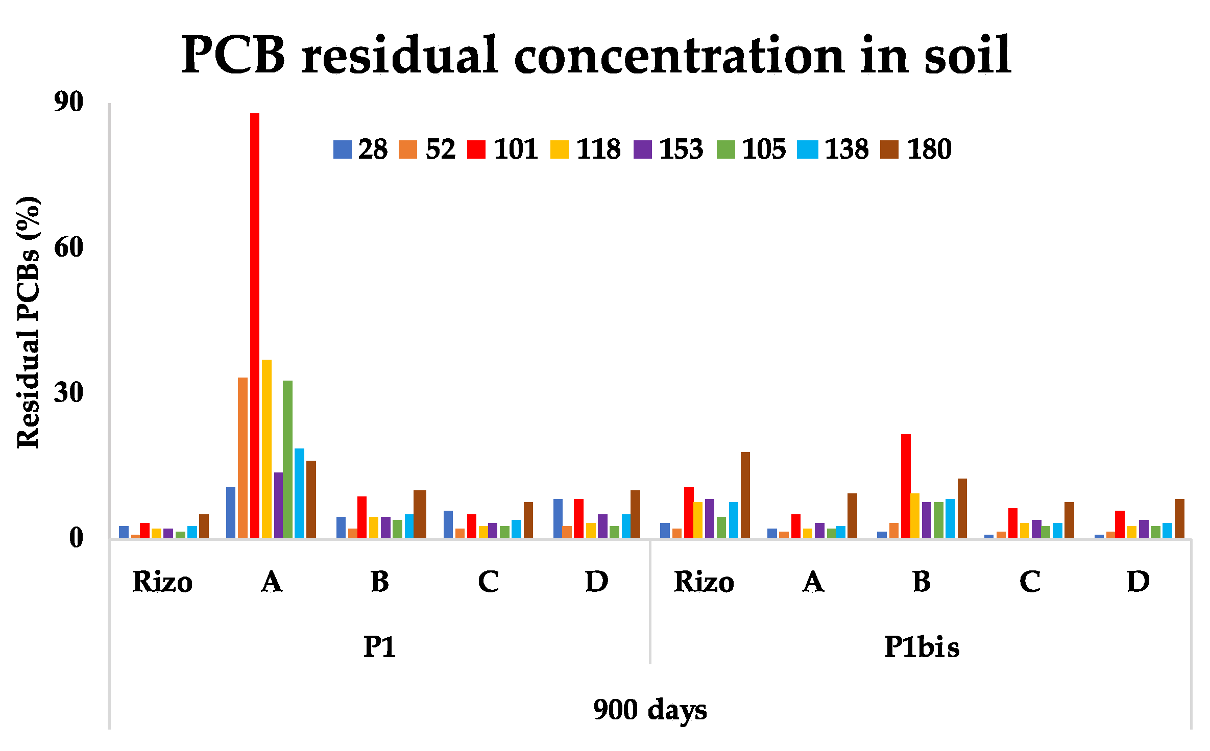
3.2.2. PCB Assessment

PCB concentrations found in the soils of the planted plots (P1 and P1bis), in the plant tissues of both target trees, and in the control soil are reported in

Table 3. Concentrations (average values (ng/g) ± standard deviation) of PCB congeners detected in: (i) soil samples at 0 day (topsoil: 0–20 cm depth) and 900 days after poplar planting. Rizo: soil surrounding the root system at 0–30 cm depth; A: 0.25 m distance from the trunk and 0–20 cm depth; B: 0.25 m distance from the trunk and 20–40 cm depth; C: 1 m distance from the trunk and 0–20 cm depth; D: 1 m distance from the trunk and 20–40 cm depth); and (ii) soil samples at 0 and 900 days taken from the control plot. Statistical differences (p < 0.001) are reported with a star symbol.

PCBs		28	52	101	118	153	105	138	180	Total
Control t = 0 d		7.65 ± 2.26	33.21 ± 9.05	92.41 ± 31.32	85.53 ± 14.11	405.76 ± 182.45	45.51 ± 4.79	273.59 ± 103.60	458.20 ± 203.22	1401.9 ± 550.8
Control t = 900 d		19.87 ± 28.16	29.56 ± 24.34	101.06 ± 71.12	108.24 ± 75.83	378.40 ± 249.50	45.62 ± 35.90	305.05 ± 193.70	406.51 ± 255.55	1394.3 ± 934.1
topsoil t = 0 d		7.25 ± 0.07	11.9 ± 0.42	10.35 ± 0.77	25.75 ± 0.35	59.75 ± 1.76	15.55 ± 1.34	73.25 ± 3.18	42.15 ± 0.77	246 ± 8.7
P1	Rizo	* 0.18 ± 0.01	* 0.07 ± 0.00	* 0.33 ± 0.05	* 0.45 ± 0.01	* 1.20 ± 0.15	* 0.23 ± 0.01	* 1.75 ± 0.25	* 2.09 ± 0.47	* 6.30 ± 1.0.
	A	* 0.75 ± 0.13	* 3.92 ± 4.16	* 9.09 ± 8.05	* 9.54 ± 7.52	* 8.28 ± 4.67	* 5.11 ± 3.66	* 13.69 ± 9.26	* 6.80 ± 1.69	* 57.2 ± 39.1
	B	* 0.33 ± 0.20	* 0.27 ± 0.12	* 0.88 ± 0.17	* 1.11 ± 0.05	* 2.82 ± 0.57	* 0.60 ± 0.02	* 3.75 ± 0.67	* 4.23 ± 0.78	* 14.0 ± 2.6
	C	* 0.42 ± 0.12	* 0.22 ± 0.09	* 0.55 ± 0.11	* 0.66 ± 0.04	* 1.90 ± 0.35	* 0.38 ± 0.03	* 2.67 ± 0.81	* 3.23 ± 0.67	* 10.0 ± 2.2
	D	* 0.58 ± 0.07	* 0.32 ± 0.04	* 0.87 ± 0.21	* 0.76 ± 0.17	* 2.97 ± 0.73	* 0.37 ± 0.04	* 3.69 ± 1.12	* 4.25 ± 1.42	* 13.8 ± 3.8
P1bis	Rizo	* 0.25 ± 0.09	* 0.27 ± 0.10	* 1.09 ± 0.16	* 1.99 ± 0.07	* 4.93 ± 0.73	* 0.71 ± 0.01	* 5.31 ± 0.35	* 7.57 ± 2.27	* 22.1 ± 3.8
	A	* 0.15 ± 0.03	* 0.14 ± 0.01	* 0.51 ± 0.01	* 0.58 ± 0.03	* 2.11 ± 0.07	* 0.31 ± 0.01	* 1.87 ± 0.07	* 4.07 ± 0.55	* 9.70 ± 0.8
	B	* 0.1 ± 0.01	* 0.40 ± 0.06	* 2.23 ± 0.67	* 2.44 ± 0.65	* 4.56 ± 1.17	* 1.19 ± 0.30	* 5.90 ± 1.68	* 5.12 ± 0.90	* 21.9 ± 5.4
	C	* 0.08 ± 0.00	* 0.16 ± 0.00	* 0.64 ± 0.00	* 0.77 ± 0.00	* 2.45 ± 0.00	* 0.41 ± 0.00	* 2.38 ± 0.00	* 3.18 ± 0.00	* 10.0 ± 0.0
	D	* 0.04 ± 0.01	* 0.14 ± 0.03	* 0.56 ± 0.03	* 0.7 ± 0.01	* 2.15 ± 0.21	* 0.38 ± 0.01	* 2.19 ± 0.13	* 3.4 ± 0.36	* 9.5 ± 0.8

. In all samples, GC–MS analyses revealed only 8 PCB congeners, such as the 6 markers (28, 52, 101, 153, 138, 180), and 2 dioxin-like congeners (118, 105); the concentrations of the other 11 congeners searched for (10 dioxin-like and 1 non-dioxin-like) were under the limit of quantification (<0.063 ng/g).

• Soils

At 900 days the total concentration of PCBs in all soil samples were below the Italian legal limit (60 ng/g, Italian Decree 152/06) and their concentrations were significantly lower than their initial values (t = 0 d, 245.95 ± 8.69 ng/g, p <0.001). In the Control soil was not observed any variation in their total amount (Table 3).

The lowest PCB content (6 ng/g) was found in the P1 Rizo, and the highest one (57 ng/g) in P1 (A) at 0–20 cm depth and at 0.25 m distance from the poplar trunk (Table 3). In particular, the highest residual PCB values in the sampling point A (0.25 m from the trunk, 0–20 cm depth) were found for the congeners 101, 118, 52, and 105 (Figure 3), suggesting that the 2 dx-like congeners (118 and 105), in addition to the other 2 markers, tend to persist in the environment. Comparing P1 and P1bis, some small differences were found between the sampling points inside each plot. For example, in P1bis, the lowest PCB concentration was found in A (9.7 ng/g), and a slightly higher amount was found in rhizosphere (22 ng/g soil).

• Plant tissues

The highest amount of PCB was found in the root system; the total amounts of PCBs were 27.7 ng/g in P1 and 27.7 ng/g in P1bis roots. Negligible concentrations of PCBs were detected in the shoots of both target plants (P1 and P1bis) (

Table 4. PCB concentrations (average values expressed as ng/g ± standard deviation) detected in plant tissues at day 900 from poplar planting.

		28	52	101	118	153	105	138	180	Total
P1	leaves	0.70 ± 0.33	0.31 ± 0.14	1.04 ± 0.10	1.06 ± 0.09	5.40 ± 0.44	0.39 ± 0.03	5.73 ± 0.25	2.62 ± 0.04	17.0 ± 0.3
	shoots	0.22 ± 0.05	0.09 ± 0.03	0.21 ± 0.06	0.12 ± 0.02	0.51 ± 0.09	0.04 ± 0.00	0.61 ± 0.10	0.39 ± 0.07	2.0 ± 0.4
	roots	2.18 ± 0.03	1.21 ± 0.10	2.48 ± 0.05	1.36 ± 0.03	8.15 ± 0.50	0.56 ± 0.03	6.94 ± 0.10	4.81 ± 0.07	28.0 ± 0.3
P1bis	leaves	0.58 ± 0.27	0.25 ± 0.11	0.96 ± 0.26	1.02 ± 0.29	4.74 ± 1.16	0.41 ± 0.14	5.08 ± 1.41	2.50 ± 0.60	15.5 ± 4.0
	shoots	0.20 ± 0.03	0.08 ± 0.02	0.21 ± 0.06	0.12 ± 0.05	0.58 ± 0.22	0.05 ± 0.01	0.54 ± 0.20	0.38 ± 0.19	2.2 ± 0.7
	roots	0.28 ± 0.04	0.17 ± 0.00	1.41 ± 0.02	1.03 ± 0.01	5.35 ± 0.05	0.49 ± 0.01	3.86 ± 0.03	3.99 ± 0.01	16.6 ± 0.1

). The PCB transport from the soil to the poplar tissues (roots or leaves) was assessed with the bioaccumulation factors (BAFs, where BAF plant part = [PCB] plant part/[PCB] soil). The calculation of the BAFs was performed considering the average value of the initial total PCBs in soil (t = 0 day) and those detected at 900 days in the rhizosphere. BAF values were quite similar in both target plants. In P1 plot, root and leaf BAF were 0.18 and 0.11, respectively; while in P1bis, BAF_root and BAF_leaf were in both cases 0.12.

The BAF value was also calculated for each single PCB congener, and very low values were obtained; the highest value (0.5) was found for the trichlorinated congener 28 in the roots of the P1 tree (Figure 4).

Finally, the transpiration stream concentration factor (TSCF) was assessed in order to evaluate the PCB translocation capability into the stem. TSCF was calculated in accordance with Terzaghi et al. [10] for the eight PCB congeners analysed; the values ranged from 1.87 × 10⁻³ to 4.12 × 10⁻⁷, confirming the low translocation of PCBs.

3.2.3. HM Evaluation in Soil

Fourteen heavy metals were investigated both in soils and in plant tissues. The initial analysis carried out (topsoil t = 0 d) in correspondence of P1 and P1bis plots before poplar plantation, revealed only 6 metals (Sn, Be, V, Ni, Zn and Cr) at concentrations exceeding the Italian legal limits for soil of industrial areas (Italian Decree 152/06).

At 900 days from poplar plantation, a significant (p < 0.05) decrease in the overall HMs was observed (

Table 5. Heavy metal concentrations (average values expressed as mg/kg ± standard deviation) detected in: (i) soil samples at 0 day (topsoil: 0–20 cm depth) and 900 days after poplar planting. Rizo: soil surrounding the root system at 0–30 cm depth; A: 0.25 m distance from the trunk and 0–20 cm depth; B: 0.25 m distance from the trunk and 20–40 cm depth; C: 1 m distance from the trunk and 0–20 cm depth; D: 1 m distance from the trunk and 20–40 cm depth) and (ii) soil samples at day 0 and day 900 taken from the control plot zone. Statistical differences (p < 0.05) are reported with a star symbol.

Italian Legal Limit (mg/kg)		Sn 1	Se 3	V 90	Ni 120	Zn 150	Cr 150
Control t = 0 d		10.5 ± 0.69	1.8 ± 0.17	61.4 ± 1.62	47.2 ± 1.60	369.68 ± 35.64	60.3 ± 1.66
Control t = 900 d		10.32 ± 2.69	1.39 ± 0.19	74.68 ± 4.66	70.65 ± 0.55	340.23 ± 31.01	79.13 ± 4.58
topsoil t = 0 d		5.96 ± 2.1	10.43 ± 2.1	127.40 ± 17.9	156.2 ± 19.3	181.28 ± 17.5	179.55 ± 20.7
P1	Rizo	* 1.53 ± 0.05	* 1.50 ± 0.14	* 61.67 ± 0.93	* 111.62 ± 2.41	* 89.65 ± 2.98	* 106.77 ± 0.67
	A	* 1.81 ± 0.07	* 1.41 ± 0.48	* 58.50 ± 0.66	* 97.84 ± 4.92	* 119.92 ± 15.24	* 104.29 ± 4.49
	B	* 1.64 ± 0.00	* 1.64 ± 0.08	* 57.77 ± 0.60	* 103.11 ± 0.20	* 99.36 ± 44.88	* 98.20 ± 0.96
	C	2.02 ± 0.63	* 1.61 ± 0.58	* 61.92 ± 5.37	* 108.23 ± 3.82	* 75.13 ± 3.04	* 105.58 ± 11.36
	D	* 1.49 ± 0.04	* 1.46 ± 0.31	* 59.56 ± 1.85	* 105.92 ± 0.86	* 76.13 ± 8.11	* 101.08 ± 2.19
P1bis	Rizo	* 1.59 ± 0.02	* 1.25 ± 0.22	* 51.13 ± 0.57	* 86.97 ± 1.65	* 73.93 ± 2.50	* 82.60 ± 0.32
	A	* 1.64 ± 0.12	* 1.59 ± 0.20	* 55.77 ± 3.80	* 83.41 ± 0.26	* 79.28 ± 3.99	* 83.32 ± 0.45
	B	* 1.67 ± 0.01	* 1.27 ± 0.21	* 50.77 ± 1.65	* 85.69 ± 2.15	* 72.96 ± 4.81	* 82.20 ± 0.53
	C	2.65 ± 1.06	* 1.52 ± 0.11	* 56.72 ± 1.96	* 88.51 ± 1.39	* 89.36 ± 5.31	* 87.97 ± 2.64
	D	* 1.83 ± 0.29	* 1.56 ± 0.09	* 52.61 ± 1.21	* 83.33 ± 1.99	* 77.93 ± 9.58	* 80.70 ± 1.47

) compared to the initial values (topsoil t = 0 d), evidencing HM concentrations under the national regulatory thresholds (Italian Decree 152/06). The only exception was Sn, whose concentration was lower than the initial one (5.68 mg/kg), but it still was above the legal limit of 1 mg/kg (Table 5). Interestingly, no reduction in HM concentrations was found in Control soils.

3.2.4. HM Evaluation in Plant Tissues

The highest concentrations of HMs observed at 900 days were in the roots with Zn > Cu > Ni > Cr > V > Pb for the P1 poplar tree and Zn > Cu > Pb > Ni > Cr > V for the P1bis poplar tree (

Table 6. Heavy metal concentrations (average values ± standard deviation) detected in plant tissues (leaves, shoots, and roots) at 900 days after poplar plantation from the P1 and P1bis plants. TF: translocation factor value for each HM.

Italian Legal Limit (mg/kg)		Sn 1	Tl 1	Be 2	Cd 2	Se 3	Sb 10	As 20	Co 20	V 90	Pb 100	Ni 120	Cu 120	Zn 150	Cr 150
P1	leaves	0.29 ± 0.26	0 ± 0.00	0 ± 0.00	0.12 ± 0.04	0 ± 0.00	0.13 ± 0.10	0.12 ± 0.03	1.83 ± 0.25	0.13 ± 0.05	0.36 ± 0.10	0.59 ± 0.29	4.62 ± 0.20	90.48 ± 2.09	0.28 ± 0.15
	shoots	0.02 ± 0.00	0 ± 0.00	0 ± 0.00	0.06 ± 0.01	0 ± 0.00	0.01 ± 0.00	0.03 ± 0.01	0.16 ± 0.03	0.03 ± 0.01	0.67 ± 0.64	4.61 ± 4.85	3.68 ± 0.44	1.5 ± 0.13	1.03 ± 1.47
	roots	0.05 ± 0.02	0.01 ± 0.00	0.02 ± 0.00	0.03 ± 0.00	0 ± 0.00	0.04 ± 0.00	0.2 ± 0.02	0.84 ± 0.02	2.75 ± 0.05	2.3 ± 0.40	7.06 ± 0.30	13.68 ± 0.33	31.4 ± 1.16	5.11 ± 0.12
	TF	5.8	0	0	4	0	3.2	0.6	2.1	0	0.1	0	0.3	2.8	0
P1bis	leaves	1.33 ± 1.32	0 ± 0.00	0 ± 0.00	0.12 ± 0.02	0 ± 0.00	0.17 ± 0.06	0.14 ± 0.03	1.47 ± 0.25	0.11 ± 0.02	0.32 ± 0.03	0.96 ± 0.45	4.57 ± 0.52	82.01 ± 14.37	0.67 ± 0.65
	shoots	0.03 ± 0.02	0 ± 0.00	0 ± 0.00	0.07 ± 0.01	0 ± 0.00	0.01 ± 0.00	0.03 ± 0.01	0.13 ± 0.01	0.04 ± 0.05	0.42 ± 0.24	0.63 ± 0.40	3.51 ± 0.16	1.51 ± 0.10	0.22 ± 0.05
	roots	0.03 ± 0.00	0.01 ± 0.00	0 ± 0.00	0.05 ± 0.00	0 ± 0.00	0.02 ± 0.01	0.12 ± 0.00	0.49 ± 0.03	1.31 ± 0.06	6.94 ± 0.72	3.91 ± 0.16	7.73 ± 0.57	29.67 ± 2.20	2.7 ± 0.22
	TF	44.3	0	0	2.4	0	8.5	1.1	3	0	0	0.2	0.6	2.7	0.2

). Zn was the most abundant metal in the leaves with values of 90.48 and 82.01 mg/kg in the P1 and P1bis plants, respectively. Overall, negligible concentrations (<1 mg/kg) of the other HMs were detected in all the plant tissues, in line with the soil results (Table 5). With regard to the shoot, Cu concentrations were higher than 3 mg/kg in both trees and Ni only in the P1 plant (4.61 mg/kg). The translocation factor (TF) (i.e., the ratio between HMs in the plant aerial part (e.g., leaves) and in the roots) was calculated for each single HM. Although TF values >1 were obtained for some elements (Sn, Cd, Sb, Co, and Zn) (Table 6), this ratio can be considered noteworthy only for Zn. In fact, in this case, the concentrations in the leaves and roots were not negligible because they were higher than 4 mg/kg.

3.3. Microbial Analysis

3.3.1. Microbial Abundance, Cell Viability

In order to assess the abundance of viable cells (No. viable cells/g soil), this was calculated by multiplying the total microbial abundance by cell viability for each sampling point datum. The microbial abundance (No. cells/g soil) and cell viability (% live/live + dead cells) at the P1 and P1bis plots (Rizo, A, B, C, D) are reported in

Table 7. Microbial abundance and cell viability of soil samples from the control, P1, and P1 bis plots at different times, ±standard errors (t = 0 and 900 days). Statistical differences (p < 0.01) are marked with a star.

PLOT	Sample	Total Microbial Abundance	Cell Viability	No of Live Cells
		No. Cells/g Soil	% Live/Live + Dead	No. Live Cells/g Soil
Control	t = 0 d	4.64 × 106 ± 5.32 × 105	54.28 ± 3.04	2.52 × 106 ± 1.62 × 104
	t = 900 d	1.54 × 105 ± 1.98 × 104	31.1 ± 4.1	4.79 × 104 ± 8.12 × 102
P1-P1bis	topsoil t = 0 d	2.11 × 107 ± 2.40 × 105	59.70 ± 6.2	1.26 × 107 ± 8.40 × 103
P1	Rizo	* 2.94 × 107 ± 3.91 × 105	* 84.82 ± 1.48	* 2.50 × 107 ± 1.21 × 104
	A	* 3.80 × 107 ± 7.07 × 105	* 76.30 ± 2.03	* 2.90 × 107 ± 8.79 × 103
	B	* 3.50 × 107 ± 5.39 × 105	* 87.05 ± 0.76	* 3.05 × 107 ± 1.31 × 104
	C	* 1.09 × 107 ± 1.01 × 106	* 81.82 ± 3.60	8.92 × 106 ± 1.64 × 104
	D	* 1.91 × 107 ± 2.67 × 105	* 68.33 ± 3.77	* 1.30 × 107 ± 5.05 × 103
P1bis	Rizo	1.90 × 107 ± 5.61 × 105	* 81.98 ± 1.50	* 1.56 × 107 ± 9.82 × 103
	A	* 1.47 × 107 ± 4.34 × 105	* 86.92 ± 0.98	* 1.28 × 107 ± 1.20 × 103
	B	* 2.76 × 107 ± 6.04 × 105	* 85.17 ± 1.94	* 2.35 × 107 ± 1.10 × 104
	C	2.06 × 107 ± 5.51 × 105	* 83.94 ± 1.02	* 1.73 × 107 ± 4.30 × 103
	D	* 3.07 × 107 ± 1.37 × 106	* 87.23 ± 1.96	* 2.68 × 107 ± 1.51 × 104

.

At day 900, the microbial abundance generally increased from its initial values (day 0) in P1 and P1 bis plots and it was always considerably higher than that of the unplanted soil (control), (Table 7).

Moreover, the cell viability increased significantly from its initial values (Krus-kall-Wallis One-way analysis of variance on ranks, p <0.01) in all the planted plots and at all depths and distance from the trunk (rhizosphere, A, B, C and D).

Moreover, considering the number of cells active in the soil (No. live cells /g soil), significantly higher values were found (Kruskall-Wallis One-way analysis of variance on ranks, p <0.01) in the rhizosphere of both planted plots and at all depths and distance from the trunk, except for C in P1.

3.3.2. Fluorescence In Situ Hybridization (FISH) Results

The characterization of the microbial community was carried out through the application of the Fluorescent In Situ Hybridization technique (FISH), using molecular probes for the identification of the main soil microbial groups. The FISH analysis was performed on rhizosphere (Rizo) and the most distant point (D) from the plant trunk (1m distance from the tree and at 20–40 cm depth) at 900 days from poplar plantation. In the P1 plot D was not directly in contact with roots, while in P1bis the roots were much more developed, reaching the D point.

The Bacteria domain was prevalent in all soil samples analysed (P1_rhizosphere: 6.5 × 10⁶ ± 6.4 × 10³; P1_D: 4.6 × 10⁶ ± 6.4 × 10³; P1bis_rhizosphere: 1.0 × 10⁷ ± 2.3 × 10⁴; P1bis_D: 1.06 × 10⁷ ± 8.9 × 10³). Archaea were also found at very low values (ranging from 3.41 × 10⁵ to 7.75 × 10⁵).

Inside the Bacteria domain, all the groups searched for were found with different numbers between P1 and P1bis and inside each plot between the rhizosphere and the D point.

The P1 plot was characterized by a dominance of Actinobacteria (3.36 × 10⁶ ± 1.78 × 10³) > Alpha-Proteobacteria (2.58 × 10⁶ ± 1.77 × 10⁶) > Firmicutes (2.31 × 10⁶ ± 7.58 × 10²) > TM7 (Candidatus Saccharibacteria, 2.08 × 10⁶ ± 3.48 × 10³) > Gamma-Proteobacteria (1.70 × 10⁶ ± 1.41 × 10³) in the rhizosphere. A significant lower number (t-test, p < 0.01) was observed at the D sampling point. In particular, Alpha-Proteobacteria, Actinobacteria, and Dehalococcoides were half of those found in the Rizo soil samples (Figure 5).

Differently, the P1bis plot did not show significant differences in the bacterial community composition between the rhizosphere and point D, in line with a higher root development.

4. Discussion

The reduction in overall PCBs under the legal limits (< 60 ng/g) in the poplar-planted plots showed the effectiveness of the Monviso clone in promoting the degradation of these persistent organic pollutants. To support this result, no variation in their values was found in the control soil (outside the poplar-treated area). These findings are in accordance with a previous sampling from the same plots; however, the total concentration of PCBs in the rhizosphere at 900 days was three times lower than that found at 420 days, in line with an increase in plant growth [15].

Our results show how root development influenced contaminant removal; in fact, in P1, where the roots tended to grow deep, the highest amount of PCBs (57 ng/g) was in the topsoil (A point), where the roots were barely detected. Differently, in P1bis the lowest PCB concentration was found in the same A point (9.7 ng/g) presumably because in this case the root development was higher and well extended on the soil surface.

PCBs in plant tissues evidenced that no accumulation occurred either in the leaves or in the roots. The only exception (BAF value > 0.5) was for the low-chlorinated PCB 28 in the P1 root. This result is in accordance with other studies that report that low-chlorinated congeners can be found in the root [15]. TSCF values confirm that PCB uptake was strongly limited due to their low bioavailability (particularly low for high-chlorinated congeners) and low dissolving in soil pore water, in accordance with Terzaghi et al. [10]. The latter authors affirm that PCB concentration found in upper-part plants (e.g., leaves) can be ascribable to soil particle deposition. In light of the PCB results at 900 days in the soils and plant tissues, it is possible to affirm that the rhizoremediation process observed at the previous sampling (420 days) is going forward.

Heavy metals cannot be degraded, but they can be transformed and made differently available and toxic by microorganisms and/or phytoextracted and/or phytocontained by plants. In the rhizosphere, synergic interactions can also occur between microorganisms and roots. For example, the presence of organic surfactants produced by both plants and bacteria can increase HM bioavailability and absorption by plants. At the same time, the soil pH can change, chelating molecules can be produced (e.g., organic acids and siderophores), and oxidation and reduction reactions occur [28,29,30].

Phytostabilization is one possible phytoremediation process, in which metal-tolerant plants halt the leaching of these molecules through the thick mat of adventitious roots and associated rhizosphere microbes [31]. The results obtained in this work suggest that the Monviso poplar clone applied was able to phytostabilize HMs. The capability of the Populus species to promote HM phytostabilization has been described by other authors [32,33]. In light of the translocation factors obtained in this work, only Zn (TF > 1) was phytoextracted by this plant; the latter result is in accordance with those found in other works [2].

The plant, thanks to different types of molecules emitted at the rhizosphere level, may have directly and indirectly stimulated some soil natural bacterial populations to transform PCBs [13,34]. In the rhizosphere, aerobic and anaerobic microhabitats can coexist, with different presences of carbonaceous sources provided by radical exudates that can favour both the degradation of low-chlorinated congeners and the anaerobic (reductive) dehalogenation of high-chlorinated ones. The analysis of the structure of the microbial community through the FISH technique showed several groups where bacteria able to transform PCBs are present. In fact, the detection of Alpha-Proteobacteria (e.g., Sphingomonas and Bradyrhizobium), Gamma-Proteobacteria (e.g., Pseudomonas, Ralstonia, and Luteibacter), Firmicutes (e.g., Bacillus, Desulfitobacterium dehalogenans, Dehalobacter, and Clostridium), Actinobacteria (e.g., Rhodococcus, Corynebacterium, and Arthrobacter), and TM7 (Candidatus saccharibacteria) [35,36,37,38,39] confirms an active role in their removal. Moreover, the presence of the genus Dehalococcoides, able to carry out reductive dehalogenation, suggests the microbial transformation of high-chlorinated congeners. The positive effect of the rhizosphere on the bacterial populations was not limited to the soil surrounding the roots, but also to those in the bulk soil close to them inside the plots. The positive “rhizosphere effect” has been described for PCB rhizoremediation by other authors [5,13] and was confirmed in our case by the increase in microbial abundance and viability in all the points of the planted plots.

Finally, inside Alpha- and Gamma-Proteobacteria and Firmicutes, there are also several species able to resist and to remove HMs [40,41].

5. Conclusions

The application of phytotechnology using the poplar Monviso clone was effective in promoting both PCB rhizodegradation and HM phytostabilization. The positive effects of the relationships between the poplar clone roots and microorganisms made possible an overall contaminant removal. Further studies are in progress in order to investigate in detail these complex interactions for improving knowledge on the “chemical dialogue” (between plants and microbes). In particular, the molecules produced by roots and bacteria able to activate the remediation processes will be studied. Understanding of the plant–microbial consortia in the rhizosphere will enhance our ability to engineer plants for phytostrategic purposes.

References

1. Ojuederie, O.B.; Babalola, O.O. Microbial and plant-assisted bioremediation of heavy metal polluted environments: A review. Int. J. Environ. Res. Public Health 2017, 14, 1504. [Google Scholar] [CrossRef] [Green Version]
2. Ancona, V.; Caracciolo, A.B.; Campanale, C.; Rascio, I.; Grenni, P.; Di Lenola, M.; Bagnuolo, G.; Uricchio, V.F. Heavy metal phytoremediation of a poplar clone in a contaminated soil in southern Italy. J. Chem. Technol. Biotechnol. 2020, 95, 940–949. [Google Scholar] [CrossRef]
3. Fiorentino, N.; Mori, M.; Cenvinzo, V.; Duri, L.G.; Gioia, L.; Visconti, D.; Fagnano, M. Assisted phytoremediation for restoring soil fertility in contaminated and degraded land. Ital. J. Agron. 2018, 13, 34–44. [Google Scholar]
4. Cristaldi, A.; Conti, G.O.; Jho, E.H.; Zuccarello, P.; Grasso, A.; Copat, C.; Ferrante, M. Phytoremediation of contaminated soils by heavy metals and PAHs. A brief review. Environ. Technol. Innov. 2017, 8, 309–326. [Google Scholar] [CrossRef]
5. Vergani, L.; Mapelli, F.; Zanardini, E.; Terzaghi, E.; Di Guardo, A.; Morosini, C.; Raspa, G.; Borin, S. Phyto-rhizoremediation of polychlorinated biphenyl contaminated soils: An outlook on plant-microbe beneficial interactions. Sci. Total Environ. 2017, 575, 1395–1406. [Google Scholar] [CrossRef]
6. Adeyinka, G.C.; Moodley, B. Kinetic and thermodynamic studies on partitioning of polychlorinated biphenyls (PCBs) between aqueous solution and modeled individual soil particle grain sizes. J. Environ. Sci. 2019, 76, 100–110. [Google Scholar] [CrossRef] [PubMed]
7. Manoj, S.R.; Karthik, C.; Kadirvelu, K.; Arulselvi, P.I.; Shanmugasundaram, T.; Bruno, B.; Rajkumar, M. Understanding the molecular mechanisms for the enhanced phytoremediation of heavy metals through plant growth promoting rhizobacteria: A review. J. Environ. Manag. 2020, 254, 109779. [Google Scholar] [CrossRef]
8. Ancona, V.; Grenni, P.; Caracciolo, A.B.; Campanale, C.; Di Lenola, M.; Rascio, I.; Uricchio, V.F.; Massacci, A. Plant-Assisted Bioremediation: An Ecological Approach for Recovering Multi-contaminated Areas. In Soil Biological Communities and Ecosystem Resilience; Lukac, M., Grenni, P., Gamboni, M., Eds.; Springer International Publishing: Cham, Switzerland, 2017; pp. 291–303. ISBN 9783319633367. [Google Scholar]
9. Passatore, L.; Rossetti, S.; Juwarkar, A.A.; Massacci, A. Phytoremediation and bioremediation of polychlorinated biphenyls (PCBs): State of knowledge and research perspectives. J. Hazard. Mater. 2014, 278, 189–202. [Google Scholar] [CrossRef] [PubMed]
10. Terzaghi, E.; Zanardini, E.; Morosini, C.; Raspa, G.; Borin, S.; Mapelli, F.; Vergani, L.; Di Guardo, A. Rhizoremediation half-lives of PCBs: Role of congener composition, organic carbon forms, bioavailability, microbial activity, plant species and soil conditions, on the prediction of fate and persistence in soil. Sci. Total Environ. 2018, 612, 544–560. [Google Scholar] [CrossRef] [PubMed]
11. Di Lenola, M.; Barra Caracciolo, A.; Grenni, P.; Ancona, V.; Rauseo, J.; Laudicina, V.A.; Uricchio, V.F.; Massacci, A. Effects of Apirolio Addition and Alfalfa and Compost Treatments on the Natural Microbial Community of a Historically PCB-Contaminated Soil. Water Air Soil Pollut. 2018, 229, 1–14. [Google Scholar] [CrossRef]
12. Nogues, I.; Grenni, P.; Di Lenola, M.; Passatore, L.; Guerriero, E.; Benedetti, P.; Massacci, A.; Rauseo, J.; Caracciolo, A.B. Microcosm experiment to assess the capacity of a poplar clone to grow in a PCB-contaminated soil. Water 2019, 11, 2220. [Google Scholar] [CrossRef] [Green Version]
13. Di Lenola, M.; Caracciolo, A.B.; Ancona, V.; Laudicina, V.A.; Garbini, G.L.; Mascolo, G.; Grenni, P. Combined Effects of Compost and Medicago Sativa in Recovery a PCB Contaminated Soil. Water 2020, 12, 860. [Google Scholar] [CrossRef] [Green Version]
14. Bianconi, D.; De Paolis, M.R.; Agnello, A.C.; Lippi, D.; Pietrini, F.; Zacchini, M.; Polcaro, C.; Donati, E.; Paris, P.; Spina, S.; et al. Field-scale rhizoremediation of a contaminated soil with hexachlorocyclohexane (HCH) isomers: The potential of poplars for environmental restoration and economical sustainability. In Handbook of Phytoremediation; Hauppauge: New York, NY, USA, 2011; pp. 1–12. ISBN 9781617287534. [Google Scholar]
15. Ancona, V.; Barra Caracciolo, A.; Grenni, P.; Di Lenola, M.; Campanale, C.; Calabrese, A.; Uricchio, V.F.; Mascolo, G.; Massacci, A. Plant-assisted bioremediation of a historically PCB and heavy metal-contaminated area in Southern Italy. N. Biotechnol. 2017, 38, 65–73. [Google Scholar] [CrossRef] [PubMed]
16. Kralj, M.; De Vittor, C.; Comici, C.; Relitti, F.; Auriemma, R.; Alabiso, G.; Del Negro, P. Recent evolution of the physical–chemical characteristics of a Site of National Interest—the Mar Piccolo of Taranto (Ionian Sea)—And changes over the last 20 years. Environ. Sci. Pollut. Res. 2016, 23, 12675–12690. [Google Scholar] [CrossRef] [PubMed]
17. Cardellicchio, N.; Buccolieri, A.; Giandomenico, S.; Lopez, L.; Pizzulli, F.; Spada, L. Organic pollutants (PAHs, PCBs) in sediments from the Mar Piccolo in Taranto (Ionian Sea, Southern Italy). Mar. Pollut. Bull. 2007, 55, 451–458. [Google Scholar] [CrossRef] [PubMed]
18. Petronio, B.M.; Cardellicchio, N.; Calace, N.; Pietroletti, M.; Pietrantonio, M.; Caliandro, L. Spatial and temporal heavy metal concentration (Cu, Pb, Zn, Hg, Fe, Mn, Hg) in sediments of the Mar Piccolo in Taranto (Ionian Sea, Italy). Water Air Soil Pollut. 2012, 223, 863–875. [Google Scholar] [CrossRef]
19. Barra Caracciolo, A.; Grenni, P.; Cupo, C.; Rossetti, S. In situ analysis of native microbial communities in complex samples with high particulate loads. FEMS Microbiol. Lett. 2005, 253, 55–58. [Google Scholar] [CrossRef] [Green Version]
20. Boulos, L.; Prévost, M.; Barbeau, B.; Coallier, J.; Desjardins, R. LIVE/DEAD(®) BacLight(TM): Application of a new rapid staining method for direct enumeration of viable and total bacteria in drinking water. J. Microbiol. Methods 1999, 37, 77–86. [Google Scholar] [CrossRef]
21. Grenni, P.; Caracciolo, A.B.; Rodríguez-Cruz, M.S.; Sánchez-Martín, M.J. Changes in the microbial activity in a soil amended with oak and pine residues and treated with linuron herbicide. Appl. Soil Ecol. 2009, 41, 2–7. [Google Scholar] [CrossRef]
22. Batani, G.; Bayer, K.; Böge, J.; Hentschel, U.; Thomas, T. Fluorescence in situ hybridization (FISH) and cell sorting of living bacteria. Sci. Rep. 2019, 9, 1–13. [Google Scholar] [CrossRef] [Green Version]
23. Pernthaler, J.; Glöckner, F.O.; Schönhuber, W.; Amann, R. Fluorescence in situ hybridization (FISH) with rRNA-targeted oligonucleotide probes. Methods Microbiol. 2001, 30, 207–226. [Google Scholar]
24. Barra Caracciolo, A.; Bustamante, M.A.; Nogues, I.; Di Lenola, M.; Luprano, M.L.; Grenni, P. Changes in microbial community structure and functioning of a semiarid soil due to the use of anaerobic digestate derived composts and rosemary plants. Geoderma 2015, 245–246, 89–97. [Google Scholar] [CrossRef]
25. Di Lenola, M.; Grenni, P.; Proença, D.N.; Morais, P.V. Comparison of two molecular methods to assess soil microbial diversity. In Soil Biological Communities and Ecosystem Resilience; Springer: Cham, Switzerland, 2017; pp. 25–42. ISBN 9783319633367. [Google Scholar]
26. Amann, R.; Fuchs, B.M. Single-cell identification in microbial communities by improved fluorescence in situ hybridization techniques. Nat. Rev. Microbiol. 2008, 6, 339–348. [Google Scholar] [CrossRef]
27. Engel, A.S.; Lee, N.; Porter, M.L.; Stern, L.A.; Bennett, P.C.; Wagner, M. Filamentous “Epsilonproteobacteria” dominate microbial mats from sulfidic cave springs. Appl. Environ. Microbiol. 2003, 69, 5503–5511. [Google Scholar] [CrossRef] [PubMed] [Green Version]
28. Uroz, S.; Calvaruso, C.; Turpault, M.P.; Frey-Klett, P. Mineral weathering by bacteria: Ecology, actors and mechanisms. Trends Microbiol. 2009, 17, 378–387. [Google Scholar] [CrossRef]
29. Wenzel, W.W. Rhizosphere processes and management in plant-assisted bioremediation (phytoremediation) of soils. Plant Soil 2009, 321, 385–408. [Google Scholar] [CrossRef]
30. Rajkumar, M.; Ae, N.; Prasad, M.N.V.; Freitas, H. Potential of siderophore-producing bacteria for improving heavy metal phytoextraction. Trends Biotechnol. 2010, 28, 142–149. [Google Scholar] [CrossRef] [PubMed]
31. Rajkumar, M.; Sandhya, S.; Prasad, M.N.V.; Freitas, H. Perspectives of plant-associated microbes in heavy metal phytoremediation. Biotechnol. Adv. 2012, 30, 1562–1574. [Google Scholar] [CrossRef]
32. Susarla, S.; McCutcheon, S.C.; Medina, V.F. Phytoremediation: An ecological solution to organic chemical contamination. Ecol. Eng. 2002, 18, 647–658. [Google Scholar] [CrossRef]
33. Yoon, J.; Cao, X.; Zhou, Q.; Ma, L.Q. Accumulation of Pb, Cu, and Zn in native plants growing on a contaminated Florida site. Sci. Total Environ. 2006, 368, 456–464. [Google Scholar] [CrossRef] [PubMed]
34. Van Aken, B.; Correa, P.A.; Schnoor, J.L. Phytoremediation of Polychlorinated Biphenyls: New Trends and Promise. Environ. Sci. Technol. 2010, 44, 2767–2776. [Google Scholar] [CrossRef] [Green Version]
35. Field, J.A.; Sierra-Alvarez, R. Microbial transformation and degradation of polychlorinated biphenyls. Environ. Pollut. 2008, 155, 1–12. [Google Scholar] [CrossRef] [PubMed]
36. Luo, W.; D’Angelo, E.M.; Coyne, M.S. Organic carbon effects on aerobic polychlorinated biphenyl removal and bacterial community composition in soils and sediments. Chemosphere 2008, 70, 364–373. [Google Scholar] [CrossRef] [PubMed]
37. Stella, T.; Covino, S.; Burianová, E.; Filipová, A.; Křesinová, Z.; Voříšková, J.; Větrovský, T.; Baldrian, P.; Cajthaml, T. Chemical and microbiological characterization of an aged PCB-contaminated soil. Sci. Total Environ. 2015, 533, 177–186. [Google Scholar] [CrossRef]
38. Leigh, M.B.; Fletcher, J.S.; Fu, X.; Schmitz, F.J. Root Turnover: An Important Source of Microbial Substrates in Rhizosphere Remediation of Recalcitrant Contaminants. Environ. Sci. Technol. 2002, 36, 1579–1583. [Google Scholar] [CrossRef]
39. Smidt, H.; de Vos, W.M. Anaerobic Microbial Dehalogenation. Annu. Rev. Microbiol. 2004, 58, 43–73. [Google Scholar] [CrossRef] [PubMed]
40. Sandaa, R.A.; Torsvik, V.; Enger, Ø.; Daae, F.L.; Castberg, T.; Hahn, D. Analysis of bacterial communities in heavy metal-contaminated soils at different levels of resolution. FEMS Microbiol. Ecol. 1999, 30, 237–251. [Google Scholar] [CrossRef]
41. Vidal, C.; Chantreuil, C.; Berge, O.; Mauré, L.; Escarré, J.; Béna, G.; Brunel, B.; Cleyet-Marel, J.C. Mesorhizobium metallidurans sp. nov., a metal-resistant symbiont of Anthyllis vulneraria growing on metallicolous soil in Languedoc, France. Int. J. Syst. Evol. Microbiol. 2009, 59, 850–855. [Google Scholar] [CrossRef] [PubMed] [Green Version]
Figure 1. Map of the experimental area planted with poplars.
Agriculture 11 00689 g001
Figure 2. Root system of P1bis target tree.
Agriculture 11 00689 g002
Figure 3. Residual percentages (%) of the various PCB congeners in soils sampled at different distances and depths from the trunk 900 days after poplar planting in the P1 and P1bis plots. Rizo: soil attached and surrounding roots, 0–30 cm depth; A: 0.25 m distance from the trunk and 0–20 cm depth; B: 0.25 m distance from the trunk and 20–40 cm depth; C: 1 m distance from the trunk and 0–20 cm depth; D: 1 m distance from the trunk and 20–40 cm depth. The percentages were calculated in relation to the initial concentration reported in Table 3.
Agriculture 11 00689 g003
Figure 4. Bioaccumulation factor (BAF, average values) of each single PCB congener calculated for leaves and roots 900 days after poplar planting in the P1 and P1bis plots.
Agriculture 11 00689 g004
Figure 5. Bacterial community structure detected by the fluorescence in situ hybridization (FISH) method at day 900 in the rhizosphere and D soil (1 m distance from the trunk and 20–40 cm depth) in the P1 and P1bis plots. ALFA = Alpha-Proteobacteria; BETA = Beta-Proteobacteria; GAMMA = Gamma-Proteobacteria; DELTA = Delta-Proteobacteria; EPS = Epsilon-Proteobacteria; Pla = Planctomycetes; CF = Cytophaga-Flavobacter; LGC = Firmicutes; HGC = Actinobacteria; TM7 = Candidatus Saccharibacteria; Dhe = Dehalococcoides, CFX = Chloroflexi.
Agriculture 11 00689 g005