Development of Thermal Performance Metrics for Direct Gas-Fired Circulating Heaters

Abstract

Many climate-controlled agricultural buildings use direct gas-fired circulating heaters (DGFCH) for supplement heat. There is no standardized test to calculate thermal efficiency for these heaters. This study aimed to develop a measurement system and analytical analysis for thermal efficiency, quantify the measurement uncertainty, and assess economics of DGFCH efficiency. The measurement system developed was similar to the ASHRAE 103 standard test stand with adaptations to connect the apparatus to the DGFCH. Two different propane measurement systems were used: input ratings < 30 kW used a mass flow system and input ratings > 30 kW used a volumetric gas meter. Three DGFCHs (21.9, 29.3, 73.3 kW) were tested to evaluate the system. Thermal efficiencies ranged from 92.4% to 100.9%. The resulting uncertainty (coverage factor of 2; ~95% Confidence Interval) ranged from 13.1% to 30.7% for input ratings of 56.3 to 11.4 kW. Key sources of uncertainty were propane and mass flow of air measurement. The economic impact of 1% difference in thermal efficiency ranged from USD $61.3 to $72.0 per heating season. Refinement of the testing system and procedures are needed to reduce the uncertainty. The application of this system will aid building designers in selection of DGFCHs for various applications.

1. Introduction

The use of Direct Gas-Fired Circulating Heaters (DGFCH) is common in climate-controlled agricultural buildings (e.g., livestock, poultry, and greenhouses) as the heating component of the thermal environment modification system. Supplemental heat is needed to achieve the environmental control goal in an agricultural setting, that is, maintain an ideal environment for the growth of the agriculture commodity with minimal cost [1]. For both animal confinement buildings and greenhouses, heating during the winter months is necessary to maintain the optimal environment and presents a significant utility cost [1,2]. In most building types, a forced air, circulating style heater is used to provide circulation of the heated air to the occupied zone within the building. Gas-fired heaters are ubiquitous due to low operating costs and fuel availability to remote locations [2]. While DGFCH are popular for agricultural applications, there are downsides in implementing them.

DGFCH are simple heaters in comparison to residential units based on the construction and operation principles. DGFCHs use a propane burner manifold placed on the intake of a blower. This does not the vent the combustion gases out of the occupied space. The output of the blower can be equipped with various directional vanes to aid in the distribution of heated air. The placement of such heaters in agricultural buildings is highly variable with no standardized placement design currently available in literature [1,3]. Thermal efficiencies of DGFCHs are commonly reported with assumed values of approximately 99%; however, the water vapor and ventilation rates of a building can decrease the thermal efficiency to 80% [4]. In comparison to residential combustion heaters, which indirectly transfer heat to the air stream via a heat exchanger and combustion gases are vented outdoors, [5]. The use of the heater exchanger reduces the thermal efficiency to a range of 65% to 80%.

DGFCHs are direct-fired, resulting in combustion gases (i.e., CO and CO₂) formed directly in the heated air. In agricultural applications, the occupied (animal or plant) spaces where DGFCHs are present are continuously ventilated, unlike residential applications. The use of DGFCHs in greenhouses could result in safety concerns for workers, if prolonged operation throughout a day is necessary due to lower ventilation rates per floor area compared to animal buildings [4]. ANSI/ASHRAE [5] define the residential furnace thermal efficiency standard; however, there is limited standard thermal efficiency testing standards and guidelines for DGFCHs. Standardization of thermal efficiency testing and calculation allow for accurate comparison of different DGFCHs designs and capacities as well as generate informative equipment design specifications to support improved supplement heat capacity sizing and layout for agricultural buildings.

There are two types (direct and indirect) of combustion tests used to determine thermal efficiency. The direct test is a measure of the enthalpy gain of the air heated by the heater. Thermal efficiency can then be determined by dividing enthalpy gain by the sum of the heating fuel gross energy and electrical energy of the blower. This ratio of energy output over energy input for a given heater is the most accurate definition of thermal efficiency as the unit must obey the conservation of energy. The indirect test is a measure of the heating value of the fuel to determine the heat output less the flue gas or combustion gas enthalpy gain [5]. There are several challenges associated with applying the indirect test methodology to evaluate DGFCHs as the flue gas is mixed with the output air. The thermal efficiency calculated with the indirect methods typically is less accurate due to measurement error. Thus, DFGCHs are most appropriately evaluated by direct test methodology.

The objectives of this study were to (1) develop and validate a testing system and analytical analysis for determining the steady-state thermal efficiency of a DGFCH through a direct testing method; (2) evaluate the testing system across a range of DGFCH units; and (3) evaluate the economics of various DGFCH for agricultural uses.

2. Materials and Methods

2.1. Thermal Efficiency

The following sections will describe the methodology used to develop a DGFCH thermal efficiency measurement system. The system was designed to accommodate a range of rated heater capacities. For development purposes, three different DGFCHs (21.9 kW (75,000 BTU h⁻¹), 29.3 kW (100,000 BTU h⁻¹), 73.3 kW (250,000 BTU h⁻¹)) were tested, procedural differences for each capacity are discussed in the testing procedure section. All tests were performed in the Air Dispersion Laboratory (ADL). See [6] for specifics of the laboratory.

2.2. Instrumentation

A Data Acquisition and Control (DAQC) system was developed to measure all necessary parameters to calculate the thermal efficiency of a DGFCH (analytical analysis to be discussed in a later section). The DAQC system consisted of two sub-systems, one to measure the input energy into the DGFCHs and one to measure the output enthalpy of the output air.

The instrumentation system for measuring input energy consisted of sensors to measure the propane input and electrical energy used by the DGFCH. Two different set-ups were created for propane input measurement. For DGFCHs rated <30 kW, a mass flow system was used, and for DGFCHs rated >30 kW, a volumetric device was used. This was performed as the minimum flow rates for traditional style diaphragm gas flowmeters exhibit high uncertainty for 30 kW rated heaters and below based on manufacturer specifications due to the extremely low flowrates. The mass flow system was not used for all heaters as the uncertainty in propane input was high, discussed in later section.

The mass flow system consisted of a 45.4 kg (100 lb) propane tank placed on a steel platform with a single-point 150 kg load cell with a 2 mV V⁻¹ linear response signal (see

Table 1. Energy input instruments used in the study in order as described in the text. FS = Full Scale.

Input Energy Instrumentation	Manufacturer’s Rating	Manufacturer’s Accuracy	Model	Manufacturer
Propane mass	150.0 kg	2.0 × 10−2% FS	RLPWM12-150 kg	Rice Lake Weighing Systems, Rice Lake, WI, USA
Programmable amplifier	NA	NA	PGA 204	Texas Instruments, Dallas, TX, USA
Propane regulator	58.6 kW	NA	Model 9059398	Char-Broil, Columbus, GA, USA
Propane flowmeter	Minimum flow = 2.8E−4 m3 s−1	4.0 × 10−5 m3 s−1	Model PGM-150	EKM Metering, Santa Barbra, CA, USA
Propane temperature	−40.0 to 150.0 °C	±0.22 °C	Model TE-IBN-D044-14	Dwyer Instruments, Inc., Michigan City, IN, USA
Propane pressure	0.0 to 103.4 kPa	1.0% FS	Model 628	Dwyer Instruments, Inc., Michigan City, IN, USA
Precision resistor	1 kΩ	±5.0 × 10−2% FS	Model 1k Tick	Labjack Corporation, Lakewood, CO, USA
Electrical power meter	Max 3000 A at 830 V AC	±0.7% of W	Model 1735	Fluke, Everett, WA, USA

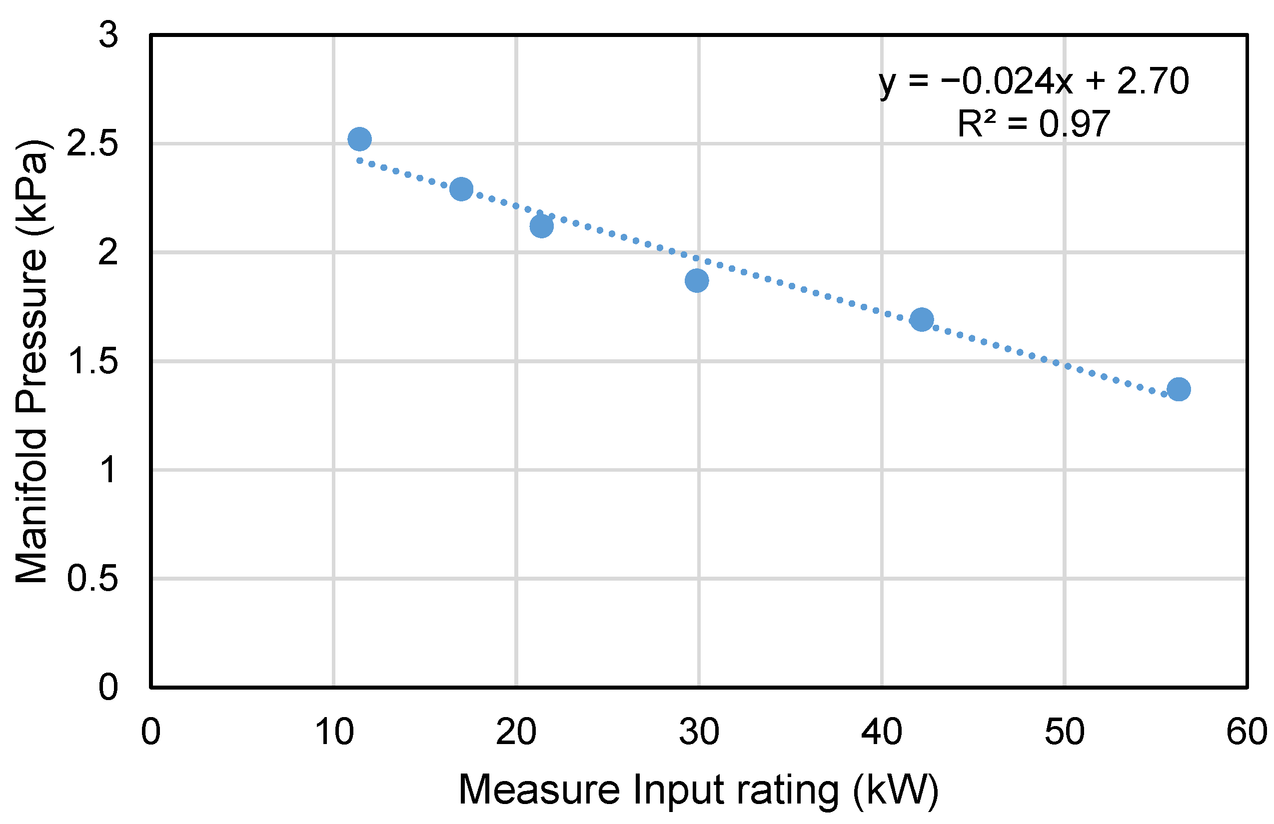
for specifications). The load cell signal was conditioned by a programmable-gain instrumentation amplifier (see Table 1 for specifications). A dual-stage regulator rated for 58.6 kW at 2.74 kPa was used (see Table 1 for specifications) with a 7.9 mm diameter flexible hose to connect the gas supply to the heater connection manifold.

The gas flowmeter (see Table 1 for specifications) was connected to the propane utility supply (two 3.79 m³ propane tanks with a line pressure of 2.74 kPa) using a 12.7 mm diameter flexible hose. The flowmeter’s output was connected to the heater connection manifold with a 12.7 mm Internal Diameter (ID) flexible hose. Flowrate was determined by dividing the difference between the recorded initial and final positions of the dial on the flowmeter by the duration of the test.

The heater connection manifold consisted of a sediment trap (following manufacturer’s recommendation) and two taps that contained a silvered PT100 Resistance Temperature Detector (RTD; see Table 1 for specifications) and a pressure transducer (see Table 1 for specifications) to monitor supply propane temperature and pressure, respectively. A precision resistor (see Table 1 for specifications) was used to create a voltage divider circuit to condition the RTD output signal with a supply voltage of 2.5 Volt DC (VDC) and the 4 to 20 mA signal from the pressure transducer. The RTD temperature was determined using the alpha equation (Equations (1) and (2)) for RTDs, with alpha determined using the resistance at 0 °C and 100 °C. Heater electrical power consumption was measured using a portable power meter (see Table 1 for specifications).

$$T_i= \raisebox{1ex}{$\left(\frac{R_T}{R_0}-1\right)$}\!\left/ \!\raisebox{-1ex}{$\alpha $}\right.$$

(1)

where

• T_i = temperature (°C); where i is RTD, propane, or exiting air
• R_T = RTD resistance at T_i (Ω) see Equation (2)
• R₀ = RTD resistance at 0 °C (100 Ω)
• α = temperature coefficient of resistance (3.851E−4 Ω °C⁻¹)

$$R_T= R_{d1}\ast \left(\frac{V_s}{V_{out}}-1\right)$$

(2)

where

• R_d1 = resistance of voltage divider resistor (1 k Ω)
• V_s = supply voltage (2.5 VDC)
• V_out = analog voltage output measured by DAQC board (VDC)

Heater combustion exhaust measurement system consisted of a 0.2 m diameter, 2.44 m long round, galvanized steel duct that contained a PT100 RTD and a velocity pressure pitot tube (Figure 1 and Figure 2,

Table 2. Dimensions of the test duct in Figure 1.

Label	Description	Measurement (m)
A	Inlet to temperature tap	1.3
B	Inlet to velocity pressure pitot tube	1.6
C	Overall length of duct	2.4
F	Duct diameter	0.2

and

Table 3. Energy output instruments used in the study in order as described in the text.

Output Energy Instrumentation	Manufacturer’s Rating	Manufacturer’s Accuracy	Model	Manufacturer
Output air temperature	−40.0 to 150.0 °C	±0.2 °C	Model TE-IBN-D044-14	Dwyer Instruments, Inc., Michigan City, IN, USA
Output air velocity pitot tube	0.5 to 51 m s−1	±2.0% FS	Model FLST-C8	Dwyer Instruments, Inc., Michigan City, IN, USA
Pitot tube pressure transducer	0.0 to 248.8 Pa	±1.0% FS	Model 267	Setra Systems, Inc., Boxborough, MA, USA
Incoming air temperature	−40.0 to 105.0 °C	±1.0% at 25 °C	Model TT05-10KC8-15-T105-1500	TEWA Sensors, LLC, Albuquerque, NM, USA
Precision resistor	10 k Ω	±5.0 × 10−2% FS	Model 10K Tick	Labjack Corporation, Lakewood, CO, USA
Incoming air temperature and relative humidity	−40.0 to 80.0 °C, 0.0 to 100.0% RH	±0.1 °C, ±1.5% RH	Model HMT120	Vaisala, Helsinki, Finland

). The same conditioning circuit and temperature equations were used as previously discussed. The supply end of the duct featured a flange fitting that was sealed with foil tape and secured to the face of the heater around the exhaust outlet. For heaters with larger output openings, a reduction flare fitting, 0.3 m to 0.2 m diameter and 0.3 m in length, was included. All seams on the inside of the duct were sealed with mastic caulking, and the outside of the duct was sealed with foil tape. The duct was wrapped with 51 mm (2 in.) thick, foil-backed fiberglass insulation. Additional insulation was placed on the seams on the fiberglass insulation, and all seams were sealed with foil tape. Velocity pressure was measured using a multi-range, differential pressure transducer (see Table 3 for specifications).

Heater supply air (room) Dry-Bulb Temperature (Tdb) was measured using a grouping of four plastic-coated thermistors (see Table 3 for specifications) installed 0.25 m below the intake of the heater on the side opposite of the Liquid Propane (LP) intake and burner manifold. The four thermistors were multiplexed (Model: CD4052BE, Texas Instruments, Dallas, TX, USA) and conditioned with a voltage divider circuit consisting of a precision resistor (see Table 3 for specifications). Temperature from the thermistors was calculated using the β equation (Equation (3)) and then converted to Celsius for analysis. The thermistors were calibrated in a variable environment chamber (Series 7064-3140, Parameter Generation & Control, Black Mountain, NC, USA) at three unique temperatures (25 °C, 35 °C, and 45 °C) using the exact same DAQC setup prior to testing. The calibration regression was developed by regressing the chamber temperature recoded from the control panel on the x-axis and the average thermistor temperature on the y-axis. The final calibration equation was determined by taking the inverse of the previous calibration equation [7].

$$T_{TRi}= 1/\left[\left(1/298.15\right)+ \left(1/\beta \right)\ast ln(\left(R_{d10}\ast \left(V_{s1}/V_{out1}-1\right)\right)/R_{ref})\right]$$

(3)

where

• T_TR = thermistor temperature i (K)
• Β = thermistor coefficient (3435)
• R_d10 = resistance of voltage divider resistor (Ω)
• V_s1 = voltage supply (5.0 VDC)
• V_out1 = analog voltage output measured by DAQC (VDC)
• R_ref = thermistor reference resistance at 25 °C (Ω)

Supply air Tdb and Relative Humidity (RH) were measured in the same location using a portable hygrometer with a Liquid Crystal Display (LCD) screen (see Table 3 for specifications). The remote hygrometer was recorded manually at the start and end of each test.

All sensors, excluding the remote sensing unit, were recorded with a custom software interface (Visual Basic v19, Microsoft, Redmond, WA, USA). The software allowed for user-selectable sampling frequency and a calibration procedure to calibrate the load cell.

2.3. Testing Procedure

Data were collected on the three nominally rated DGFCHs (21, 29, and 73 kW) at the full rated output and half output setting. For the 21 and 29 kW rated heaters, three replicates of each output were measured. For the 73 kW heater, two replicates of each output were completed. This was due to issues with the test duct retaining residual heat between tests. Prior to test initiation, the load cell was verified with a 45.4 kg (100 lb) standard set of weights. During a test, the DAQC was configured to sample continuously at 1 Hz. For DGFCH ratings > 18 kW, the total sampling duration was 500 s with the DAQC system sampling at 1 Hz. For DGFCH ratings < 18 kW, the total sampling duration was 900 s, with the DAQC sampling at 1 Hz. The time duration was different for the heater and settings rated for <18 kW based on the anticipated propane consumption to have a minimum change in the propane tank mass double the load cells accuracy. Electrical energy consumption was recorded from the power meter at 3 min into the test and assumed constant for the duration of the test. The three-minute mark was selected based on ANSI/ASHRAE Standard 103, considering steady-state combustion at three minutes [5]. Between performance tests, the ADL was ventilated for 60 min to maintain similar room temperatures at the start of each test.

2.4. Thermal Efficiency Development

The energy balance of a DGFCH is the balance of the energy input and output of the heater (Equation (4)). Output DGFCH energy can be defined as the sum of the combustion heat in the output airflow and the radiative and convective heat loss of the heater jacket (Equation (5)). For agriculture buildings, the main objective is to warm the occupied zones of the house. Thus, the goal of a DGFCH thermal efficiency is to quantify the efficiency of heating the output air (Equation (6); [5]).

$$Q_{out }= Q_{in}$$

(4)

where

• Q_out = energy output of a direct gas-fired circulating heater (kW)
• Q_in = energy input (propane and electrical) of a direct gas-fired circulating heater (kW)

$$Q_{out }= Q_a+ Q_j$$

(5)

where

• Q_a = energy output via air (kW)
• Q_j = energy output via heater jacket (kW)

$${\widehat{Q}}_{out }= Q_{in}\times {ɲ}_{ss}$$

(6)

where

• ${\widehat{Q}}_{out }$ = measured energy output of heater output air (full or half load; kW)
• ${ɲ}_{ss}$ = steady-state sensible energy output efficiency (%)

Energy input into a DGFCH can be quantified as the energy from the liquid propane plus the electrical energy (Equation (7)). Electrical energy is included as most of the DGFCH supply air is drawn in over the motor and electronic components for cooling purposes. For the 21 and 29 kW rated heaters, input propane was measured gravimetrically, while input propane for the 73 kW rated heater was measured volumetrically, with a temperature and pressure compensated gas meter.

$$Q_{in}=\left({\dot{x}}_{LPG}\times HH{V}_{prop}\right)+W_{elec}$$

(7)

where

• ${\dot{x}}_{LPG}$ = mass flow rate of propane to heater (kg s⁻¹) or volume flow rate of propane (m³ s⁻¹)
• HHV_prop = higher heating value of propane (kJ kg or kJ m⁻³)
• W_elec = electrical energy consumption of heater (kW)

$${\widehat{Q}}_{out}= {\dot{m}}_a\times \left(h_{out }- h_{in}\right)$$

(8)

where

• ${\dot{m}}_a$ = mass flow rate of exhaust air from heater (kg s⁻¹)
• h_out = enthalpy of output air from heater (kJ kg⁻¹)
• h_in = enthalpy of oncoming air to heater (kJ kg⁻¹)

$${\dot{m}}_a= \stackrel{\rightharpoonup }{V}\times \left(\pi r^2\right)\times \rho$$

(9)

where

• $\stackrel{\rightharpoonup }{V}$ = fluid velocity (m s⁻¹)
• r = radius of the duct (0.10 m)
• $\rho$ = density of the air exiting heater (kg m⁻³)

$$\stackrel{\rightharpoonup }{V}=\sqrt{\frac{2\delta p}{\rho }}$$

(10)

where

• δp = velocity pressure measurement (Pa)

The output energy was quantified by the enthalpy change of the air moving through the heater (Equation (8)). The mass flow of the DGFCH exhaust air was calculated using the density measurements and the pitot tube measurement (Equations (9) and (10)). The specific volume and enthalpy were calculated using the humidity ratio of the starting room conditions [1,8]

By combining the input energy (Equation (4)) and the quantified energy output (Equation (5)), the steady-state thermal efficiency can be solved for the DGFCH (Equations (11) and (12)). The thermal efficiency equation is similar in nature to efficiency equations used to evaluate solar air heaters [9,10]

$${\dot{m}}_a\times \left(h_{out }- h_{in}\right)= \left(\left({\dot{x}}_{prop}\times HH{V}_{prop}\right)+W_{elec }\right)\times {ɲ}_{ss}$$

(11)

$${ɲ}_{ss}= \dot{(m_a}\times \left(h_{out }- h_{in}\right))÷\left(\left({\dot{x}}_{prop}\times HH{V}_{prop}\right)+W_{elec}\right)$$

(12)

2.5. Thermal Efficiency Calculations and Analysis

From each replicate, the mean of six random sub-samples of 30 s (n = 30 per sub-sample) of consecutive data was used to calculate the steady-state thermal efficiency (Equation (12)). A moving average of five data points was used to reduce fluctuations in the output air temperature. This processing step was justified due to the random error caused by turbulence and non-constant combustion of the heater. The mass flow rate of the propane was calculated by determining the weight change of the propane cylinder divided by the experiment duration. For DGFCH’s rated >18 kW, a 4 s average before the heater solenoid was opened and after the test was used to determine the pre- and post-weight. For DGFCH’s rated <18 kW, a 3 s average was used. The averaging of the cylinder weight was necessary to account for variation in the weight caused by vibration of the cylinder due to propane flow.

A sensitivity analysis of the steady-state thermal efficiency was performed with respect to the Higher Heating Value (HHV) of propane. Four sources of the HHV were used in the analysis due to the slight differences among sources (

Table 4. Higher Heating Value (HHV) values from different sources used in the sensitivity analysis of the thermal efficiency equation.

Source	HHV (kJ kg−1)	References
A	50,009	[5]
B	50,411	[8]
C	50,656	[11]
D	50,129	[12]

).

2.6. Uncertainty Analysis

The final standard uncertainty of the thermal efficiency (Δ${ɲ}_{ss}$) was calculated from the standard uncertainty obtained from all key measurement inputs propagated through (Equation (13) through Equation (20), Figure 3).

A zeroth-ordered uncertainty budget was created for each measured input: voltage measurement for exiting air temperature (T_ex;

Table 5. Uncertainty budget analog voltage measurement by DAQC board for RTD measurement.

.	Value (VDC)	Probability Distribution	Divisor	Standard Uncertainty (Pa)
Accuracy [a]	3.7 × 10−3	Rectangular	$\sqrt{3}$	2.1 × 10−3
Quantization error [b]	3.1 × 10−4	Rectangular	$\sqrt{3}$	1.8 × 10−4
Combined standard sensor uncertainty, ΔVDC				2.1 × 10−3

^[a] ±0.5 Manufacturer’s stated accuracy with ±5. VDC input range. ^[b] ±0.5 ADC resolution = 14-bit ADC resolution, ±5 VDC reference range = 3.1E−4 V BL⁻¹. BL = Binary Level.

), a Differential Pressure Transducer (DPT;

Table 6. Uncertainty budget for differential pressure transducer.

Source	Value (Pa)	Probability Distribution	Divisor	Standard Uncertainty (Pa)
Accuracy RSS [a]	2.5	Rectangular	$\sqrt{3}$	1.4
Long-term stability	5.0	Rectangular	$\sqrt{3}$	2.9
Quantization error [b]	3.2 × 10−2	Rectangular	$\sqrt{3}$	1.8 × 10−2
Combined standard sensor uncertainty, Δδp				3.2

^[a] Root sum square (at constant t_db), ±1.0% full scale (δp1) 0 to 248.8 Pa; ^[b] ±0.5 sensor resolution = (14-bit ADC resolution, ±10 VDC reference range = 6.1E−4 V BL⁻¹) (sensor sensitivity)⁻¹.

), dry-bulb temperature, and relative humidity for humidity ratio calculation (Tdb and RH;

Table 7. Uncertainty budget for temperature and relative humidity sensor used to calculate humidity ratio.

Source	Value (°C, %RH)	Probability Distribution	Divisor	Standard Uncertainty (°C, %RH)
Accuracy RSS [a]	0.1, 1.5	Rectangular	$\sqrt{3}$	5.7 × 10−2, 8.7 × 10−1
Long-term stability	N/A [c], 1.0	Rectangular	$\sqrt{3}$	N/A [c], 5.7 × 10−1
Display Resolution [b]	5.0 × 10−3, 5.0 × 10−3	Rectangular	$\sqrt{3}$	2.9 × 10−3, 2.9 × 10−3
Combined standard sensor uncertainty, Δtdb, Δrh				5.7 × 10−2, 1.0

^[a] Manufacturer stated accuracy; ^[b] ±0.5 smallest display value = 0.01; ^[c] long-term stability is included in accuracy term from manufacturer specifications.

), propane flow for mass and volumetric ($\dot{x}$;

Table 8. Uncertainty budget for propane for both mass and flow basis.

Source	Value (kg, m3 s−1)	Probability Distribution	Divisor	Standard Uncertainty (kg, m3 s−1)
Accuracy RSS [a]	1.0 × 10−2, 4.4 × 10−4	Rectangular	$\sqrt{3}$	5.7 × 10−2, 2.6 × 10−4
Long-term stability	N/A [c], N/A [c]	Rectangular	$\sqrt{3}$	N/A [c], N/A [c]
Display Resolution [b]	N/A, 1.4 × 10−3	Rectangular	$\sqrt{3}$	NA, 2.5 × 10−3
Quantization Error [d]	6.1 × 10−3, N/A	Rectangular	$\sqrt{3}$	3.5 × 10−3, N/A
Combined standard sensor uncertainty, $\Delta {\dot{x}}_m, \Delta {\dot{x}}_f$				5.8 × 10−2, 2.4 × 10−3

^[a] Manufacturer stated accuracy; ^[b] ±0.5 smallest display value = 0.01; ^[c] long-term stability is included in accuracy term from manufacturer specifications; ^[d] ±0.5 sensor resolution = (14-bit ADC resolution, 1 VDC reference range = 1.2E−4 V BL⁻¹) (sensor sensitivity)⁻¹.

), and electrical energy consumption (W_elec;

Table 9. Uncertainty budget for electrical energy consumption of the heater.

Source	Value (W)	Probability Distribution	Divisor	Standard Uncertainty (W)
Intrinsic error	241.5	Rectangular	$\sqrt{3}$	139.4
Operating error	517.5	Rectangular	$\sqrt{3}$	298.8
Display Resolution [a]	50	Rectangular	$\sqrt{3}$	28.9
Combined standard sensor uncertainty, ΔWelec				331.0

^[a] ±0.5 smallest display value = 50.

) and included the manufacturer’s accuracy and long-term stability, quantization error from the 14-bit Analog-to-Digital Converter (ADC), and the Standard Error (SE) from the experimental data (SE was removed from the budget as it changes with each experiment; [13]).

The uncertainty budget for the Tdb and RH includes a display resolution component as it was manually recorded (Table 7). The propane volumetric measurement also had a display resolution component from the dial on the meter display from manually recording measurements.

The standard uncertainty associated with the area of the duct was determined by propagating the standard uncertainty of the duct radius (Δr = 2.70 × 10⁻³ m, one-half the reading resolution set by the manufacturer) through the area equation of a circle resulting in a standard uncertainty of the area Δa = 3.39 × 10⁻³ m².

$$\Delta VD{C}_i^2={\left(\frac{\Delta VDC}{n}\right)}^2 +S{E}^2$$

(13)

where

• ΔVDC_i = combined standard uncertainty in analog voltage measurement (T_ex VDC)
• SE = standard error of the voltage measurement (VDC)

$$\Delta T_{ex}^2={\left(\frac{\partial T_{ex}}{\partial VDC} \Delta VD{C}_i\right)}^2+ {\left(\frac{\partial T_{ex}}{\partial R_{d1}} \Delta R_{d1}\right)}^2+ {\left(\frac{\partial T_{ex}}{\partial R_{ref}} \Delta R_{ref}\right)}^2+RMS{E}^2$$

(14)

where

• ΔT_ent = combined standard uncertainty in entering air temperature (°C)
• ΔR_d1 = 1 kΩ resistor in divider circuit (±0.05%; Ω; rectangular distribution)
• ΔR_ref = 100 Ω at 0 °C (±0.12%; Ω; rectangular distribution)
• RMSE = root mean square error from nonlinear regression (°C)

The standard uncertainty of the entering temperature measured by the thermistor did not include propagation of uncertainty through (Equation (3)) as the DAQC system was identical in both calibration and testing. Thus, it was assumed that the RMSE of the calibration encompasses the uncertainty associated with the measurements propagated through the equation.

$$\Delta T_{ent}^2= AC{C}^2+RMS{E}^2+ S{E}^2$$

(15)

where

• ΔT_ent = combined standard uncertainty in entering air temperature (°C)
• ACC = manufacturer’s accuracy (±0.2 °C; rectangular distribution)
• RMSE = root mean square error from linear calibration regression (°C)
• SE = standard error of the mean (°C)

$$\Delta W^2={\left(\frac{\partial W}{\partial t_{db}} \Delta t_{db}\right)}^2+{\left(\frac{\partial \rho }{\partial rh} \Delta rh\right)}^2$$

(16)

where

• ΔW = combined standard uncertainty in humidity ratio (kg_H2O kg_da⁻¹)

$$\Delta {\rho }^2={\left(\frac{\partial \rho }{\partial t_{ex}} \Delta t_{ex}\right)}^2+{\left(\frac{\partial \rho }{\partial W} \Delta W\right)}^2$$

(17)

where

• Δρ = combined standard uncertainty in moist air density (kg m⁻³)

The standard uncertainty in the mass flow (Equation (18)) was determined from the propagation of the velocity pressure uncertainty, density uncertainty, area uncertainty, and accuracy of the pitot tube system.

$$\Delta {\dot{ma}}^2={\left(\frac{\partial \dot{ma}}{\partial dp} \Delta dp\right)}^2+{\left(\frac{\partial \dot{ma}}{\partial \rho } \Delta \rho \right)}^2+{\left(\frac{\partial \dot{ma}}{\partial a}\Delta a\right)}^2+AC{C}_v{}^2$$

(18)

where

• Δ$\dot{ma}$ = combined standard uncertainty in mass flow moist air (kg s⁻¹)
• ACC_v = accuracy of the velocity measurement (1.0%, [5])

$$\Delta h_{ex-ent}{}^2={\left(\frac{\partial h_{out-in}}{\partial W} \Delta W\right)}^2+{\left(\frac{\partial h_{out-in}}{\partial T_{ent}} \Delta T_{ent}\right)}^2+{\left(\frac{\partial h_{out-in}}{\partial T_{ex}}\Delta T_{ex}\right)}^2$$

(19)

where

• Δ$h_{out-in}$ = combined standard uncertainty in change in enthalpy (kJ kg⁻¹)

The standard uncertainty of ${\dot{x}}_{LPG}$ included in (Equation (20)) included the SE term for the initial and final measurement from the gravimetric system as a multi-second average was used. It was assumed that there was no uncertainty in the run time of each test factored into ${\dot{x}}_{LPG}$.

$$\Delta {ɲ}_{ss}{}^2={\left(\frac{\partial {ɲ}_{ss}}{\partial \dot{ma}} \Delta \dot{ma}\right)}^2+{\left(\frac{\partial {ɲ}_{ss}}{\partial h_{ex-ent}} \Delta h_{ex-ent}\right)}^2+{\left(\frac{\partial {ɲ}_{ss}}{\partial \dot{x}}\Delta {\dot{x}}_{LPG}\right)}^2+ {\left(\frac{\partial {ɲ}_{ss}}{\partial W_{elec}}\Delta W_{elec}\right)}^2$$

(20)

where

• Δ${ɲ}_{ss}$ = combined standard uncertainty in thermal efficiency (%)

The combined standard uncertainty was calculated using the data from each replicate of the heater model and output setting. Thus, for each replicate and output, a standard deviation was calculated for the uncertainty due to variations in measurements between each replicate.

2.7. Economics of Heater Efficiency

Economic implications of heating agricultural buildings were assessed by modifying the degree-day heating method (Equation (21); [3]). The method is simpler than other heating cost methods that use binned ambient weather data, with the consequence of overestimating the heating season costs. The efficiency represents the Annual Fuel Energy Use Efficiency (AFEUE). The AFEUE is based on the ASHRAE standard 103 [5]. For DGFCH without a pilot light, the AFEUE is the same as the steady-state thermal efficiency. For a DGFCH with a pilot light, the calculation of AFEUE considers the proportion of time with the pilot light on and its efficiency over the duration of the heating season.

$$E= C_D\times \left[\left( H_L\times D \times S \right)÷\left(\Delta t \times {ɲ}_{ss/AEU} \times HH{V}_{prop} \right)\right]$$

(21)

where

• E = propane usage per season (kg)
• C_D = correction factor for degree-days (0.6)
• H_L = design heating load at minimum ventilation (kW)
• D = degree-days (°C day)
• S = seconds per day (86,400 s d⁻¹)
• Δt = design temperature difference, inside/outside (°C)
• HHV_prop = higher heating value for propane (kJ kg⁻¹)

The calculation of the heating load for a building (heat gain/heat loss) was developed to account for the wide variety of building specifications (Equation (22)). This was performed by accounting for the heat gain on the basis of floor area. The heating load is to be calculated at the wintertime 99% design temperature for the given location.

$$HL= \left[\left(UA\times \Delta T\right)+\left(\dot{V_b }÷ \upsilon \times C_p\times \Delta T\right) \right]+ \left[q_g \times A_f\right]$$

(22)

where

• UA = overall building heat loss coefficient (W °C⁻¹)
• $\dot{V_b }$ = minimum ventilation rate (m³ s⁻¹)
• υ = specific volume of air/water mixture (kg m⁻³)
• C_p = specific heat of air (J kg⁻¹)
• Q_g = heat production per unit of floor area (W m⁻²)
• A_f = floor area of building (m²)

A sensitivity analysis of the energy usage (Equation (21)) was performed based on recommended thermal resistance (R values) for various building components, internal design temperature, two different minimum ventilation rates, and heater efficiency. This analysis used a high heat gain per unit floor area of 1.6 W m⁻². It was assumed that the outside design temperature was −29 °C (99% heating value for Minnesota; [8]). For this economic analysis, the building size was 45.7 m (L), 15.2 m (W) with a 2.5 m ceiling (150 ft L, 50 ft W with 8 ft ceiling). The building’s thermal analysis assumed no windows and doors and did not include any perimeter or floor heat loss. The R values, internal building temperature, and minimum ventilation rates (

Table 10. Sensitivity analysis inputs for R values, internal building temperature, and minimum ventilation rate. Recommended levels of insulation for homes based on climate [3].

Level of Insulation	Wall (R m2 °C W−1)	Ceiling (R m2 °C W−1)
UAlow	2.1	3.5
UAmedium	2.5	4.4
UAhigh	3.5	5.8
UAultra-high	3.5	6.7
Design internal temperature
Tihigh = 28 °C	Timedium = 25 °C	Tilow = 20 °C
Minimum ventilation rate
	Vhigh = 6 ACH [a]	Vlow = 3 ACH [a]

^[a] ACH = air changes per hour.

). For the analysis of the first three components (level of insulation, design internal Tdb, and minimum ventilation rate), the heater efficiency was 99%, and the cost of propane was assumed at USD $0.53 kg⁻¹ ($1 gallon⁻¹).

3. Results and Discussion

3.1. Thermal Efficiency

The average values of the operational parameters and results for the three DGFCHs tested at each output performed as expected (

Table 11. Average (standard deviation) of test conditions and measured performance values for all three DGFCH models and outputs.

Measured Input [a] (kW)	Heater Model	Manifold Pressure (kPa)	Output Air Temperature (°C)	Enthalpy Gain (kJ kg da−1)	Volumetric Output (L min−1)	Thermal Efficiency [b] (%)
11.43	A	2.5 (3.0 × 10−2)	67.2 (2.0)	51.2 (1.1)	13,198 (51)	94.3% (1.5)
17.00	B	2.3 (3.0 × 10−2)	80.0 (1.2)	61.9 (0.4)	16,352 (33)	92.4% (1.5)
21.39	A	2.1 (6.0 × 10−2)	118.3 (1.4)	102.1 (1.1)	14,631 (401)	96.5% (1.5)
29.89	B	1.9 (5.0 × 10−2)	140.8 (1.0)	125.5 (0.6)	17,169 (242)	94.98% (1.1)
42.20	C	1.7 (3.0 × 10−2)	131.0 (1.6)	109.2 (0.5)	29,019 (93)	100.9% (0.3)
56.27	C	1.4 (3.0 × 10−2)	180.4 (2.3)	159.1 (3.6)	29,439 (200)	98.8% (2.0)

^[a] Measured input calculated using HHV from [5]. ^[b] Thermal efficiency calculated using HHV from [5].

). The procedures developed were capable of detecting the relatively small differences in input and output energy, although the 73 kW did not reach rated operation. The time to steady-state assumed from ASHRAE 103 was represented in the results of this study (Figure 4), with all heaters and replicates showing similar trends in temperature change over time. Future tests should involve a high accuracy CO and O₂ sensor to verify the thermal efficiency through stoichiometry (indirect combustion test). A unique trend was noted in the comparison of the half and full output thermal efficiencies. Heater models A and B exhibited higher thermal efficiencies at full output, while heater model C exhibited a higher thermal efficiency at half output. The thermal efficiency of over 100% is related to the system’s uncertainty, discussed in the next section. The general trend of efficiency increasing with heater output could be influenced by the test stand gaining heat during the test and affecting measurements. This was the reason behind two replicates with heater model C. The heater models used in the study had limited thermal efficiency values reported, model A had no reported values, and models B and C reported 99.99% thermal efficiency. The reported thermal efficiencies in this study are higher than what is assumed for DGFCH in buildings 80%, with high humidity and low ventilation [4]. However, it was not within the scope of this study to evaluate the heaters under such conditions that are believed to drastically reduce the performance of these heaters in buildings. The thermal efficiency of the DGFCH used in this study is significantly higher (>90%) compared to the thermal efficiency of common gas-fired residential units (63% to 44%; [13]). This drastic difference is mainly contributed to the difference in the heaters as the residential heaters.

The measured input energy to heater model C at full output was significantly lower than its nominal rating of 73.3 kW. Upon investigation of the operational parameters of the tests, it was noted that manifold pressure exhibits a negative trend in relation to the measured input (Figure 5). The temperature of the propane did not vary between any heaters and replicates. This is most likely caused by an improper design of the propane supply of ADL that limits the maximum output due to propane flow and not the heater reaching its rated output.

The sensitivity analysis of the thermal efficiency equation in relation to the HHV was performed for heater model A at full output. The maximum difference noted in the analysis is between HHV source A (97.3%) and D/C (96.0%), with source B (96.5%) falling in-between. While all four sources are relatively similar in value, this highlights the differences in reported values among groups (sources A, B, C) and the federal government (source D). A unified HHV between all organizations is imperative to avoid discrepancies in design and in the rating of all types of propane combustion heaters.

3.2. Uncertainty Analysis

The expanded (coverage factor = 2; ~95% confidence interval) uncertainty ranged from 13.1% (Standard Deviation; SD = 0.1%) to 30.7% (SD = 8.0%) for the input energy rating 56.3 to 11.4 kW; the SD is from the multiple replicates of each heater output tested. There is a distinct difference in the variability of the uncertainty between the replications for a heater based on the propane measurement system. The mass flow system had significantly greater variability (Figure 6). The breakdown of the uncertainty contributions (

Table 12. Expanded uncertainty component contributions for Equation (20) based on the propane measurement system. The values in parentheses represent 1 standard deviation of the mean.

	Airflow	Change in Enthalpy	Propane Flow	Electrical Consumption
Mass flow	38.0% (14.3)	4.0% (3.0)	55.9% (16.2)	2.1% (1.4)
Volumetric Flow	80.8% (4.9)	17.5% (4.5)	0.6% (0.2)	1.2% (0.3)

) demonstrates that for the mass flow system, the propane mass flow and air mass flow are the largest contributors while using volumetric flow measurement, the air mass flow, and change in enthalpy are the largest contributors. Overcoming the variability in the propane mass flow for future tests could require a hardware-based signal conditioning filter to account for the signal noise due to vibrations. Alternatively, extended test duration could be used to reduce variability.

The expanded uncertainty component contributions for the volumetric propane measurement system suggest that if a high accuracy, low flow rate option was feasible, it would reduce the uncertainty considerably. To reduce uncertainty in future experiments, a higher-accuracy pressure transducer and RTD would be warranted.

3.3. Economics of Heater Efficiency

The economic estimates for heating the specified building using design conditions show a wide heating cost for a heating season (

Table 13. Economic analysis (values reported in USD) for a general agricultural building for a heating season with a heat production of 1.6 W m⁻².

	Vhigh			Vlow
Level on Insulation	Tihigh	Timedium	Tilow	Tihigh	Timedium	Tilow
UAlow	$7059	$6756	$6260	$3844	$3676	$3398
UAmedium	$6941	$6644	$6159	$3727	$3564	$3297
UAhigh	$6794	$6505	$6032	$3579	$3424	$3170
UAvery high	$6762	$6475	$6005	$3548	$3395	$3144

). There are a few limitations to the degree-day method for estimating this cost. First, it assumes a constant balance temperature for a building. Balance temperature is the ambient temperature that separates the need for heating or cooling, which is different for the various types of agricultural buildings (livestock versus greenhouse). For livestock buildings, this approach cannot account for the increase in the animal’s heat production through a growth cycle and the change in sensible heat production with indoor temperature. This economic assessment confirms that the greatest heating cost factor is the minimum ventilation rate, with building internal temperature and insulation level being the other factors impacting cost. It should be cautioned against decreasing the ventilation rate of a building to reduce the seasonal heating cost as air quality and moisture levels will be directly impacted and could negatively impact production within the building. The costs and corresponding energy inputs are higher than reported values from field studies for animal agricultural buildings with similar heat production values per floor area [14,15,16]. These differences are most likely attributed to the method used and the local weather data differences from the reported study’s locations.

The sensitivity analysis for the scenario regarding heater efficiency (

Table 14. Economic cost (values reported in USD) of reducing the DGFCH thermal efficiency by 1% for a heating season.

Level on Insulation	Tihigh	Timedium	Tilow
UAlow	$72.0	$68.9	$63.9
UAmedium	$70.8	$67.8	$62.8
UAhigh	$69.3	$66.4	$61.6
UAvery high	$69.0	$66.1	$61.3

) shows the economic impact of reducing the DGFCH thermal efficiency by 1% for the combinations of internal temperature and building envelope insulation level. The range of costs is caused by the different range of supplemental heat needs based on internal temperature and insulation value. The magnitude of the costs would be significantly higher if an AEU efficiency for a heater with a pilot light.

The methods used to perform this economic analysis could be adapted to a range of scenarios to evaluate utility costs for building types, climates, and construction for a cost estimate. Other methods for estimating heating costs are binning methods, where data is binned by day for heating demand (time and temperature difference). This method has advantages in being able to incorporate livestock heat production curves and variable ventilation rates. The downside is that this method requires extensive calculations for each time period within each day and is not a simple calculation for agriculture professions to estimate heating costs for a building.

4. Conclusions

A custom testing apparatus and instrumentation system were developed and evaluated for Direct Gas-Fired Circulating Heaters (DGFCH) commonly used in agricultural buildings. Three DGFCH were used for the evaluation testing of the system. The steady-state thermal efficiency of the tests was determined using data from the testing system and based on calculations from a standard for residential systems [5]. An uncertainty analysis was performed on the thermal efficiency calculation for the given measured inputs. An economic analysis for heating common agricultural buildings was performed. An inadequate propane service limited the systems testing ability for 73 kW rated heaters. A sensitivity analysis of the thermal efficiency in respect to the Higher Heating Value (HHV) results in a maximum difference between sources of HHV of 1.3% efficiency. This highlights the need for standardization between all organizations involved. The uncertainty of the system ranged from 13.1% to 30.7% across the input range of 56.2 to 11.4 kW, respectively. The propane mass was the key source of uncertainty at the lower ratings. A more robust hardware system and longer run times would reduce this key source of uncertainty. At higher input ratings, the mass flow of air was the key source of uncertainty. Reducing this would require the use of higher-accuracy sensors. The economic analysis showed that for a 1% difference in heater efficiency across the combination of inputs (insulation and inside temperature), the costs per heating season ranges from USD $61.3 to $72.0. Future evolutions of this system are needed to reduce the overall uncertainty in thermal efficiency. It is suggested that a flowmeter with lower minimum flow ratings be used or longer test durations to reduce the main source of uncertainty. Other instrumentation improvements are needed for the output air and velocity measurement in the duct. Overall this system shows a great prospect for testing DGFCH commonly used in agricultural buildings. This study has highlighted the need for standardized procedures for quantifying DGFCH thermal efficiency specific to agricultural applications. The unique nature of these heaters presents challenges for testing and has a large economic impact on the agricultural operation during heating seasons.

References

1. Albright, L.D. Environment Control for Animals and Plants; American Society of Agricultural and Biological Engineers: St. Joesph, MI, USA, 1990; ISBN 0-929355-08-3. [Google Scholar]
2. Cui, Y.; Theo, E.; Gurler, T.; Su, Y.; Saffa, R. A Comprehensive Review on Renewable and Sustainable Heating Systems for Poultry Farming. Int. J. Low Carbon Technol. 2020, 15, 121–142. [Google Scholar] [CrossRef]
3. Midwest Plan Service. Structures and Environment Handbook; MWPS-1-TSM; Midwest Plan Service: Ames, IA, USA, 1983. [Google Scholar]
4. Sanford, S. Greenhouse Unit Heaters—Types, Placement & Efficiency; University of Wisconsin Cooperative Extension: Madison, WI, USA, 2011; p. 6. [Google Scholar]
5. ANSI/ASHRAE. Method of Testing for Annual Utilization Efficiency of Residential Central Furnances and Boilers; ASHRAE: Atlanta, GA, USA, 2017. [Google Scholar]
6. Hoff, S.J.; Utrecht, D.V.; Harmon, J.D.; Mangold, D.W. A General Purpose Laboratory for Evaluating Livestock Ventilation Systems. Appl. Eng. Agric. 2000, 16, 701–710. [Google Scholar] [CrossRef]
7. Doebelin, E.O. Measurement Systems: Application and Design, 5th ed.; McGraw-Hill: New York, NY, USA, 2004; ISBN 0-07-243886-X. [Google Scholar]
8. ASHRAE. ASHRAE Handbook; ASHRAE: Atlanta, GA, USA, 2013. [Google Scholar]
9. Parker, B.F.; Lindley, M.R.; Colliver, D.G.; Murphy, W.E. Thermal Performance of Three Solar Air Heaters. Sol. Energy 1993, 51, 467–479. [Google Scholar] [CrossRef]
10. Saxena, A.; Verma, P.; Srivastava, G.; Kishore, N. Design and Thermal Performance Evaluation of an Air Heater with Low Cost Thermal Energy Storage. Appl. Therm. Eng. 2020, 167, 114768. [Google Scholar] [CrossRef]
11. Energy Information Administration (EIA). EIA Energy Units and Calculators Explained—U.S. Available online: https://www.eia.gov/energyexplained/units-and-calculators/ (accessed on 21 January 2021).
12. REGO. LP—Gas Serviceman’s Manual; REGO: Elon, NC, USA, 2020. [Google Scholar]
13. Juanicó, L.E.; González, A.D. Thermal Efficiency of Natural Gas Balanced-Flue Space Heaters: Measurements for Commercial Devices. Energy Build. 2008, 40, 1067–1073. [Google Scholar] [CrossRef]
14. Sharpe, K.T.; Reese, M.H.; Buchanan, E.S.; Tallaksen, J.E.; Janni, K.A.; Johnston, L.J. Electrical and Thermal Energy Consumption in Midwest Commercial Swine Facilities. Appl. Eng. Agric. 2018, 34, 857–864. [Google Scholar] [CrossRef]
15. Barber, E.M.; Classen, H.L.; Thacker, P.A. Energy Use in the Production and Housing of Poultry and Swine—An Overview. Can. J. Anim. Sci. 1989, 69, 7–21. [Google Scholar] [CrossRef]
16. Fernandez, M.D.; Losada, E.; Ortega, J.A.; Arango, T.; Ginzo-Villamayor, M.J.; Besteiro, R.; Lamosa, S.; Barrasa, M.; Rodriguez, M.R. Energy, Production and Environmental Characteristics of a Conventional Weaned Piglet Farm in North West Spain. Agronomy 2020, 10, 902. [Google Scholar] [CrossRef]
Figure 1. Test duct with locations of temperature measurement taps (D) and velocity pressure pitot tube (E). Measurements for the specific labels are in Table 1. Note diagram is not to scale.
Agriculture 11 00588 g001
Figure 2. Test stand configuration and DAQC system in ADL for DGFCH test.
Agriculture 11 00588 g002
Figure 3. Fishbone diagram of the final standard uncertainty in the thermal efficiency calculation. Each line represents the integration of a measurement and its respective uncertainty into a standard uncertainty calculation.
Agriculture 11 00588 g003
Figure 4. Temperature gain of the exiting air over the course of a test for heater model A at full output.
Agriculture 11 00588 g004
Figure 5. Measured input of propane (x-axis) versus the manifold propane pressure (y-axis).
Agriculture 11 00588 g005
Figure 6. Expanded thermal efficiency (y-axis) versus heater input rating (x-axis). The blue circles represent the measurements using the mass flow system, and the red squares represent the volumetric flow measurements.
Agriculture 11 00588 g006