1. Introduction
Agriculture has undergone substantial changes in the past, which has been named the structural change [
1], including several dimensions: the decrease of its share in the economy, both in terms of income and employment, changes in technology, labour characteristics, ownership and financing patterns, internal and external linkages and farm size. Notwithstanding the difficulty of finding a commonly agreed definition of structural change [
2], the economic literature has widely debated the determinants of the structural change, which have been indicated as changes in demand following income growth, changes in relative sectoral prices due to different technological progress, demographic and human capital factors, changes in input–output linkages and off-farm employment opportunities, changes in advantage via globalisation and international trade and resource mobility [
3,
4,
5]. Regardless of the determinants, the most visible structural change is represented within the sector by a declining number of farms and an increase in average farm size. This is the issue this paper specifically addresses. The increase in firm size is also a common feature of the evolution of the industrial and services sector as a consequence of emerging economies of scale. However, in these sectors, it can take the form of both the birth and growth of new firms and the merging of existing firms. In agriculture, such processes find a critical constraint in the limitedness of land, a fundamental production factor that cannot be produced. Hence, the entry of a new farm, or the growth of an already existing one, is largely conditional on the exit of an existing farm. The structural evolution of agriculture therefore follows specific paths, where what is of interest here is exactly the modality and the pace of the change. The decrease in the number of farms is indeed not generally accompanied by a corresponding decrease in farmed land. For instance, in the 2007–2014 period, the number of farms in the EU-28 decreased by 24.2 percent, while the utilised agricultural area (UAA) decreased by just 0.2 percent [
6]. With few exceptions, the decrease in the number of farms was for all member countries largely greater than the decline in the UAA. In Italy, in the 2000–2010 period that we considered in our empirical exercise, the number of farms decreased by 32.3 percent, a strong acceleration relative to the 1990–2000 period, when the decrease rate was only 15.8 percent. This raises the issue of the reasons for the acceleration, given that during the 2000–2010 decade, there were no evident general conditions factors that could justify such a change. Retirement programs for farmers were operating in the CAP framework since the preceding decade and the general retirement laws (“Dini reform” in 1995 and “Maroni reform” in 2004) delayed the age of retirement (which should have also reduced the farm exits linked to retirement). As to the national economic environment, it was a decade of stagnation, notwithstanding the 2007 crisis did not initially strongly hit Italy, the value added only increased by 4 percent in real terms in the whole decade, and the real agricultural value added decreased by 4 percent. Hence, there were no strong apparent factors pulling farmers out of the sector, neither in terms of employment attraction nor in terms of increasing income differentials. The reasons for the trend in the number of farms that produced a 44 percent increase in the average UAA (from 5.4 to 7.9 ha), as compared to the 4.2 percent in the preceding decade, are therefore important to investigate.
On the issues of the structural change and the way the agricultural sector reacts and adapts to changing economic conditions, two issues are at stake: land use and farm size changes. The former is relevant for the use of the territory, where the main concerns are land abandonment and non-agricultural use of land as a competitor to agriculture. The latter is relevant for the efficiency and the profitability of the sector, which mainly depends on the existence of economies of scale in farming. Changes in farm size obviously depend on the relative rapidity of changes in the number of farms and in the farmed area.
The literature on these topics covers two separate streams. One considers the factors of agricultural land changes, while the other has examined the determinants of exits from the sector. While there is an obvious connection between the two issues, they have not been considered together in a unified framework. The destiny of a farm, i.e., the technical-economic production unit, is not the same as the destiny of the farm operator. In addition, the family business nature of the majority of farms in both developing and developed countries adds complexity to the interplay between farmer exit, farm exit and land-use change. The desire for continuity of the family farm is traditionally part of the farming culture in most countries. This translates to the possibility that farm continuity enters into the objective functions of farmers, thus influencing their behaviour and their reaction to economic shocks.
In this paper, we present a conceptual framework of the evolution of the number of farms and land use that produces the conclusion that a major determinant of the change in the number of farms is the presence or absence of successors of ageing farmers and that these socio-demographic variables are the most relevant for the evolution of the sector in terms of farm size, though they do not significantly affect the changes in the farmed area. We empirically support our theoretical framework using econometric analysis of the determinants of the change in the number of farms and the farmed area with reference to an Italian Region, namely, Piedmont.
In the following section, we shortly review the literature on the above topics. Then, we present our conceptual framework. The data used for our estimations are presented in
Section 4. The relevant econometric approach and the results are illustrated in
Section 5 and discussed in
Section 6. Some concluding considerations are given in
Section 7.
2. Literature Review
The issue of structural evolution calls for the determinants of agricultural land change and the determinants of farm exits and entries. Agricultural land abandonment has increased since the 1950s [
7], which has risen globally, especially in parts of North and South America, and in Europe [
8], particularly in mountainous areas [
9]. The abandonment of agricultural land can have environmental and social negative effects, such as a reduction in landscape heterogeneity, increased fire frequency, soil erosion and desertification, biodiversity loss and loss of cultural and aesthetic values, but possibly also benefits, e.g., revegetation and forest plantations, water retention and soil recovery, along with nutrient cycling, and an increase in biodiversity [
10,
11]. A substantial literature considers the determinants of the abandonment of agricultural land (for literature reviews, see [
10,
12]). Regarding determinants of farmland abandonment, this literature commonly identifies both biophysical characteristics of the land, and socio-economic characteristics, which were also classified by Terres et al. [
13] under three headings, namely, regional context, unsuitable environmental conditions and low farm stability and viability. Among the first group, which are generally identified through remote sensing tools, the considered variables are, e.g., elevation, low soil productivity, steepness, climate and irrigation [
14]. Socio-economic and regional characteristics are related to farming opportunity costs and relative rural location attractiveness and may include farm size and fragmentation, population density, agricultural and off-farm income, distance from cities, road infrastructures, farmers’ ages, etc. The relationship between the determinants and farmland abandonment is analysed at an aggregated region, state, or municipality levels (one exception is Yan et al. [
15], who use individual plots). Many studies use logit or probit models for which a 0/1 variable indicating farm area decrease represents the dependent variable, or regressions for which the area change is the dependent variable. The literature reviews cited above are consistent in indicating that the socio-economic determinants are more important than the biophysical and environmental ones.
Land abandonment and the farm exit process are strictly connected and, in many cases, the two phenomena are interrelated. The entry–exit process is a very important factor in agriculture since it is crucial in determining farm size. Given the non-reproducibility of land, an increase in farm size is almost only possible at the expense of other existing farms. The entry–exit process is believed to allow for maintaining the global competitiveness and viability of the agricultural sector [
16,
17]. The entry–exit process of farms in the United States has been analysed using U.S. Census data [
18], finding that the farm operator’s age, economic trends and part-time occupation were the most important variables in the entry–exit farm process. Pietola et al. [
19] analysed the timing and types of farm exits, pointing out that farmer’s age, farm size, land price and retirements benefits influenced the farm exits. Farm profitability, and hence high agricultural prices, are another factor that obviously lowers the probability of farm exit [
16]. These are common findings, as several studies show that larger farms and younger farm operators are associated with a lower probability of exit [
20,
21,
22]. In addition to this, in a recent study, Landi et al. [
23] also add the effects of farm location, in particular, population density in non-urban areas. A further element that is considered to influence exits is part-time farming, with contrasting results. It is a long-lasting discussion, and still undecided, whether part-time is a step towards an exit from agriculture or helpful for remaining in farming and on which is the role of pluriactivity in farm succession [
24,
25]. The operator’s pluriactivity could suggest a family choice of exiting from farming in the long run or a permanent and stable situation. The empirical results are mixed. Weiss [
26], Stiglbauer and Weiss [
27] and Simeone [
28] found that part-time farming lowers the probability of family succession, while Kimhi and Nachlieli [
29] and Breustedt and Glauben [
16] found opposite results. Corsi [
30] distinguished between principal vs. secondary off-farm occupation, the former favouring the presence of successors, unlike the latter. Policy support for agriculture has also been shown to count. In areas where high subsidy payments are more widespread, the exit rates of farms are the lowest [
16]. This last result was previously confirmed by other studies on farm business survival, which highlighted the importance of direct and high subsidy payments, institutional constraints on land transactions [
31] and farm-supporting programs in preventing a farm exit [
32]. Another stream of research pointed out the role of social drivers, such as human capital and off-farm job opportunities and income, as well the growth of the non-agricultural economy, in playing important roles in reducing farm exits [
16,
33].
A final related issue to be considered is the fact that most entries into farming are due to inheritance. Intergenerational transfer of farms prevails in many countries [
34,
35,
36] and this is specific to the agricultural sector. Laband and Lentz [
37] and Lenz and Laband [
38] note that the rate of occupational inheritance among farmers is greater (up to five times) than it is among other categories. Regardless of the several theories trying to explain the mechanisms of intergenerational transmission (for a review, see Corsi [
39]), this is evidence of either a preference or an economic advantage of intra-familiar farm transfer.
3. Conceptual Framework
The above literature does not unify the change in the number of farms and the change in farmed land into a single framework. Most of the above literature on farm exits models them as the result of a maximising behaviour by individual farmers comparing their expected income from quitting to continuing farming. The models are mostly drawn from Todaro’s [
40] model of labour migration, which was extended by Barkley [
41]. This is the starting point of our reasoning. We first considered the farmer’s propensity to stop farming. According to the models of farm exit as drawn from the migration models, the farmer compares the utility of their farm activity to the utility of an alternative off-farm income, weighted by the probability of finding a job, and quits farming if the latter is greater than the former. In the real world in the context of developed countries, the farmer quits farming only if a real job opportunity materialises after a job search. One can posit that a farmer that is still of working age decides to start searching if the expected benefits from the search, weighted by the subjective probability that the search is successful, are greater than the (out-of-pocket and subjective) search costs. Alternatively, their willingness to actively search for an alternative job in order to quit farming can be assumed to depend on their perception of the adequateness of farm income. Adequateness here can be intended in terms of minimum survival income requirements and the spirit of Simon’s [
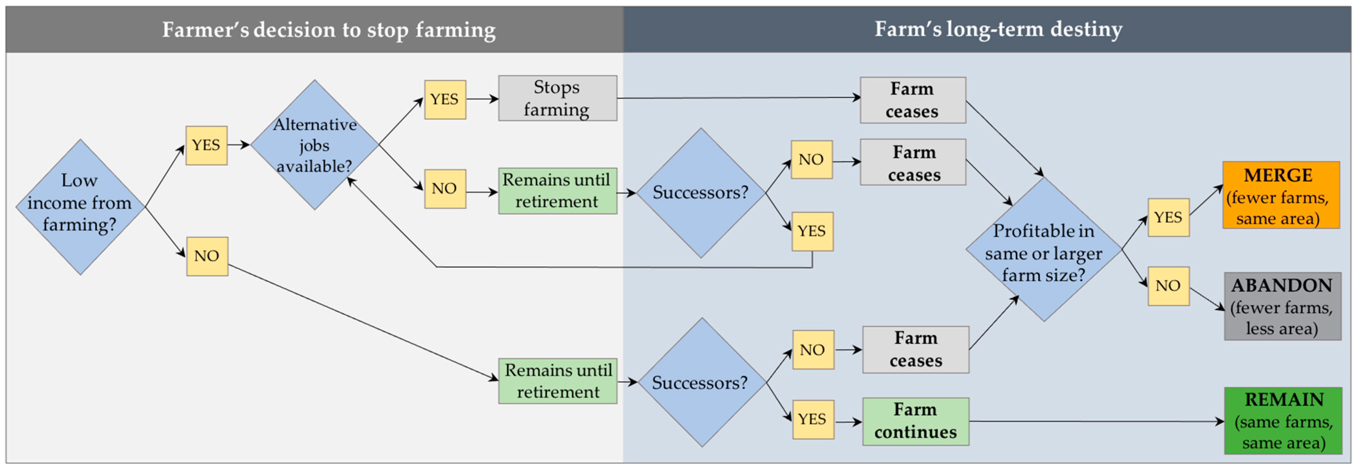
42] satisficing behaviour. That is, the farmer has a subjective aspiration income threshold to reach, below which they choose the alternative of searching for another job. The threshold is subjectively but also socially determined, that is, it depends on the average income levels and the availability of jobs in the area. Either way, the actual decision to quit farming is conditional on the realisation of an alternative job opportunity. If this happens, then the farmer actually quits. By contrast, if the operator has no alternative job opportunity, they may maintain the farm operation since, in this case, their labour opportunity cost is low and subjective. If selling or renting the farm to a neighbour is unattractive because the income it provides is low, then the farmer remains until the age of retirement, provided that the farm yields a minimum survival income. It should be specified that in the above discussion, “alternative job opportunity” has to be understood as an occupation that excludes the possibility to farm. Hence, part-time farming is not considered here as an alternative to farming since it does not have an immediate consequence on the farm continuity, though it might have an effect in the long term.
According to this model, the probability that a farmer decides to start searching for an alternative job or to consider retirement can be empirically represented by a dichotomous variable W, taking the value 1 if the farmer decides to stop farming, 0 otherwise. W is an inverse function of utility from farming (F), comprising utility from the farm income and psychological benefits; a direct function of the potential income and psychological benefits from alternative occupations (O) or from retirement (R); a function of the available job opportunities (J).
F is a function of all variables affecting the farm’s profitability (farm size s, the physical productivity y, the general profitability of the specific farming sector p and the operator’s ability because of their human capital h) and the farmer’s other personal characteristics h influencing their farm income and their preference for farming. O is influenced by the average non-agricultural wage level (w) and by the farmer’s other personal characteristics h influencing their off-farm income and their preference for off-farm jobs. R depends on the farmer being of a retirement age (a) and receiving a retirement treatment t. Available job opportunities (J) can be represented by variables describing the local labour market (l), such as activity and unemployment rates, but are also a function of the farmer’s human capital h.
The probability that a farmer of working age will actually quit (Q = 1) depends on the probability of the materialisation of actual job opportunities (depending on local labour market conditions l and on the farmer’s personal human capital h), conditional on the farmer’s willingness to start searching:
In reduced form, the probability of quitting is therefore:
While this is equivalent to the empirical implementations of the models in the literature on farm exits, it is important to note that the actual farmers’ behaviour as depicted here is different from the one assumed in the labour migration models, in which the decision to migrate is not conditional on the actual materialisation of a job.
Moreover, the models of farm exits do not consider the destiny of the farm subsequent to the choice of exiting or not. Consider the situation of a farm whose operator decides to quit farming. Indeed, the farm the farmer leaves can either be taken over as such by a family member or by a new operator, or used to enlarge an already existing close farm, or abandoned. In the first two cases, the number of farms and the farmed area remain unchanged. In the third, the number of farms declines but the farmed area does not. In the fourth, both the number and the area decrease. The results of these outcomes are obviously different in terms of the average farm size and, to the extent that economies of scale operate, in terms of the efficiency of the sector. However, they are also different in terms of the configuration of the territory and the social fabric. It is therefore important to analyse and compare the determinants of the change in the number of farms and the change in the farmed area.
In this process, an important further element that is linked to the family nature of most farms has to be considered. Farm continuity can be an important issue when farming is a family tradition such that it may enter into the utility function, possibly counterbalancing the economic advantages of quitting farming. This brings the issue of farm succession to the forefront, which is crucial for the future of the farm. It makes a difference with the process of firm growth in the other sectors, where firms can grow both based on internal growth and on mergers and acquisitions. Internal growth is constrained for farms (except for intensification) due to the scarcity of land, whose total amount is given or can be adjusted only marginally, conditional on land availability at a reasonable distance from the existing farm. Hence, having other farms ceasing their activity is a precondition for farm enlargement, where the crucial issue is not whether the individual farmer stops farming but whether the farm stops being operated at its present size.
From this point of view, family succession is crucial. Let us examine different situations and their prospects. The link between the farmer’s decision to start searching for an alternative job and quit farming and the farm’s destiny is graphically synthetised in
Figure 1.
Consider first a farm with low returns but whose operator has no alternative job opportunity such that they maintain the farm operation until the age of retirement. When they retire, one possibility is that a family member takes over the farm operation. In general, the literature suggests that the higher the farm income, the more likely it is for an intra-family succession to occur ([
27,
29,
30,
43,
44,
45]; for a review, see Corsi [
39]). This implies that low-income farms are also those where most likely no potential successor lives, though this by no means excludes that “rich” farms also have no successor [
30]. Farm continuity is also more likely if a successor is working on the farm, possibly combining farm work with an off-farm occupation, while a lack of successor makes disruption in farm continuity more likely. If there is no family successor, the final destination of the farm depends on the general economic conditions of agriculture in the area. If income prospects are poor, even for larger farms, the result will be abandonment, whereas in the opposite case, the farm will be sold or rented to neighbouring farms such that a reduction in the number of farms and growth in the average farm size will result.
Consider now a farm providing a sufficiently high income to make the farmer prefer continuing farming, even if alternative off-farm jobs are available. Then, the farmer has an incentive to remain until their retirement but if they have no successor in the family, they will eventually quit and the farm will change hands. The farm can then remain the same with a new operator, but it could also be acquired by neighbouring farms. Therefore, in this case, the lack of successors increases the probability of farm consolidation and hence a reduction in the number of farms, even with good profitability, while it does not affect the farmed area.
Therefore, the probability that the farm stops operating in its present size (X), conditional on the farmer being willing to stop farming, depends on the absence of successors (ns) and the farm’s profitability Z (which depends on the farm size s, the physical productivity y and the general profitability of the specific farming sector p) affecting the attractiveness of the existing farm for a new operator:
and hence:
By averaging the individual probabilities over a specific territory (in our case, the municipality), one obtains the mean predicted change in the total number of farms. This is the base for the empirical strategy for estimating the determinants of the change in the total number of farms.
Unlike the probability of farm closure, the probability of land abandonment (A) only depends on the long-term profitability of land, even when considering possible economies of scale, regardless of the presence of a successor. This is because what is at stake for the abandonment is not whether the farm remains at the same size after the farmer quits, but whether someone else takes it or it is merged with another farm. Note that poor income prospects for farming, which reduce the probability of having a successor for the farm and favour the exit of existing farms, also depresses the demand from new entrants and neighbouring farmers, thus leading to land abandonment. From this point of view, specific natural conditions affecting the profitability of land are crucial. The probability of land abandonment is therefore a function of the physical productivity y, the general profitability of the specific farming sector p and possibly the farm size s (as an indicator of potential economies of scale):
and hence:
Note that though the variables affecting land abandonment are the same as the ones affecting the change in the number of farms, their strengths are predictably weaker since the latter are a precondition but not a direct determinant of land abandonment. In other words, the reduction in farmed area in our framework only concerns those low-income farms in marginal areas where farming is not profitable, even with larger farm sizes. Hence, the effect of the lack of successors on the farmed area change, if any, can be expected to be weak. By contrast, the lack of successors favours the end of operation of both low-income and high-income farms. Therefore, it influences the change in the number of farms rather than the change in the farmed area. The effect of the lack of successors, and more generally of the variables affecting both the change in the number of farms and the change in the farmed area, is expected to be greater in terms of the number of farms than in terms of land change.
Our hypothesis on the functioning of the structural change process can therefore be empirically tested by examining which variables affect the change in the number of farms and the farmed area, as well as their strength.
4. Data and Methodology
Our empirical strategy was to verify the hypothesis that farm succession is an important determinant of the structural change by analysing the determinants of the change in the number of farms and the farmed area, including among the explanatory variables the absence of family successors. Ideally, one would want to use individual farm data, following the operator’s and farm’s destiny over time. Unfortunately, such data are not easily available, especially considering the long time that would be needed. We therefore used aggregated data at the municipality level of an Italian Region, namely, Piedmont, to analyse the rates of change of the number of farms and the utilised agricultural area (UAA) between the Agricultural Censuses of 2000 and 2010.
The data for our analysis were drawn from microdata of the Agricultural Censuses of 2000 and 2010 for Piedmont that were made available by the regional authority. Piedmont is located in the north-west of Italy. Though traditionally an industrial region, it has a sizeable agriculture sector that is dedicated to both commodities (cereals, fruits, dairy) and specialties (especially wine). It also has quite a diversified territory, from plains to mountains. It is therefore an interesting case study.
We could access the individual farm recordings of the Censuses. Unfortunately, the Census data for the two years could not be matched, and it was not possible to detect whether a farm of the first Census was present at the second one to analyse the destiny of each farm. It was therefore necessary to use aggregated data and to analyse net changes rather than actual entries and exits, but the high number of municipalities allowed for a quite detailed analysis at the territorial level, which is an advantage in that it avoids using aggregations that are too large.
After discarding the few farms whose total agricultural area (TAA) was 0, there were 106,149 farms recorded in 2000 and 67,062 in 2010. In some farms (936 in 2000 and 820 in 2010, corresponding to 0.9 and 1.2 percent of the total number, respectively), the head of the farm was neither the operator nor a relative; therefore, they were not family farms. Though they were few, in 2000, they had a substantial share (15.4%) of the utilised agricultural area (UAA) and an even larger share of the TAA (24.1%). Both the UAA and the TAA of non-family farms decreased dramatically between 2000 and 2010, by 54.7 and 45.3 percent, respectively. Within the family farm sample, the number of farms decreased between 2000 and 2010 by 37 percent, their TAA remained constant and the UAA increased slightly by 3.6 percent, hence their average size increased. This slight increase in the UAA was most likely due either to the merging of farms and the resulting elimination of duplicate non-farmed areas dedicated to facilities or the merging of non-family farms into family farms; the variation of the UAA decrease rate across municipalities in the utilised sample was nevertheless large, as the coefficient of variation was 96.74.
Table 1 presents the data on the number, UAA and TAA by the elevation zone (plain, hill, mountain) and by the type of farming (TF) (the EU Farm Accounting Data Network (FADN) defines a farm as specialised in a TF if the standard gross margin (SGM) for the particular production covers more than two-thirds of the total SGM [
46]; SGMs are obtained based on the farm area (number of heads) of a crop (livestock) and the area-specific (livestock-specific) standardised gross margins). It can be noted that the variation in the number of farms was roughly the same for the total of farms and the family farms, but the UAA of specialist grazing livestock TF increased by 2.7% during the decade for all farms, but by 47.2% for family farms; in the same way, the TAA for the same TF decreases by 8.3%, while it increased by 39.9% for family farms.
When looking at elevation zones, the variation in the UAA was of the same magnitude for family and non-family farms in hills and plains (−4.5% and −4.9% in hills; +6% and +5% in plains, respectively). Nevertheless, in the mountains, it increased by 13.1% for family farms, as opposed to a decrease by 62.7% for non-family farms. Similar trends were found for TAA: its variations in the mountains were +4.7% and −49.2% for family and non-family farms, respectively; +6.5% and −14.6% in the plains; in the hills, by contrast, the decrease was higher for family farms (−10.1% vs. −1.2%). Overall, it is evident that there was a transfer of land to the sector of family farms, particularly in specialist grazing livestock TF and in the mountains. This complicated the analysis of the influence of family and operators’ characteristics on the exit processes since for non-family farms, succession was not an issue, and the family, demographic and personal characteristics variables were arguably less important. We therefore focused the analysis on the data that was calculated for family farms only (referred to as the family farms database), but we add in
Appendix A the estimates of data calculated for the overall population of farms (all farms database). The analysis was therefore focussed on the sector of family farms, but some reference will be made to the analysis based on the database of the overall population of farms.
The individual farm data were aggregated into averages at the municipal level to provide the explanatory variables and we calculated the change rates in the number of farm, UAA and TAA, which were the dependent variables. Discarding the municipalities where in either year no family farm was present, we obtained 1193 observations (by municipalities) since in some cases, in either Census year, only non-family farms were recorded. When considering the whole population of farms, 1196 municipalities could be evaluated.
The relevant explanatory variables for our purpose were the indicators of the likelihood of intra-family succession. The individual Agricultural Census data classified household members as “Spouse”; “Other cohabitant household members”, separately for those working and not working on the farm; “Other operator’s relatives working on the farm”. Unfortunately, the data did not report the kinship to the operator of the last two categories. We defined a “child” as someone belonging to one of the two last categories and of a generation (at least 18 years) younger than the operator. We argue that a child living and working on the farm is a good indicator of the possibility of an intra-family succession; more so if they worked full-time on the farm.
Based on these assumptions, different indicators of the absence of possible successors in family farms were calculated, characterised by the decreasing likelihood of an intra-family succession. For each farm, we inspected the presence/absence of the different categories of successors, and for each municipality, we calculated the share of farms whose operator in 2000 was older than 55 (such that in the 10 years between the two Censuses, they would reach retirement age) and in which a successor of the four below categories was absent. The first category (NO_SUC_SHR) was the absence in the farm household of a cohabitant child working full-time on the farm. The second (NO_SUC_SHR2) was the absence of a cohabitant child working on the farm regardless of whether their work was full-time or part-time. This is a weaker indicator of the likelihood of farm succession since working part-time on the farm suggests a weaker commitment to the farm operation. The third indicator (NO_SUC_SHR3) marked those farms that not only had no cohabitant child working full-time or part-time on the farm, but not even a non-cohabitant child working full-time on the farm. We nevertheless only illustrate the results with the first category, the results of the other categories are reported in
Appendix B.
To assess whether operators’ average characteristics affected the change in the number of farms and the UAA, some explanatory variables concerned farmers’ characteristics possibly influencing farm income due to their human capital or their preference for farming. They were the average operators’ age, the share of male operators, the average operators’ education in years (the Census only reports the maximum schooling level reached by the operators; we transformed this variable into years of schooling under the hypothesis of regular attendance) and the share of operators with an education in the agricultural field (in high school or university). The share of farm households with very small (0–5 years old) or small (6–13 years old) children was also included to assess whether the presence of young generations favours the willingness to maintain the farm. This could be due to the long-term prospect of farm succession or to adjustments in labour use in the household to care for young children.
In addition, we considered the part-time status of operators. From the individual farm data, we identified the farms where the operator worked off the farm in two modalities, namely, as the principal or secondary occupation. We then calculated the shares of farms with operators in either situation at the municipality level.
Another economic determinant of farm exits (which, in our framework, was a determinant of the willingness to search for an alternative job) that is usually found in the literature is farm size. As an indicator of farm economic size, we took the standard gross margin (SGM). SGMs are defined by the Farm Accounting Data Network (FADN) of the European Union based on the farm area (number of heads) of a crop (livestock) and the area-specific (livestock-specific) standardised gross margins. SGM has the advantage of not depending on the physical farm size, which can be questionable because of different intensities and because of animal productions. We experimented with the mean SGM of each municipality but we eventually preferred to use the median SGM, a measure not affected by outliers, though the results did not sensibly differ between the two variables.
To proxy the physical environment that can affect land productivity and hence the probability of land abandonment, we considered two variables. An indicator was the elevation zone of the municipality. The modalities were mountain, hill and plain areas, where the last was used as the reference, considering that natural conditions are more unfavourable in the hills and even more so in the mountains relative to the plains. This was probably a poor representation of the differences across individual farms since, for instance, farms in the same municipality defined as mountainous may be differently productive if located in valley floors or on high slopes, but it was sufficiently good on the aggregate. Another considered indicator was the ratio between the UAA and the TAA, where a higher ratio obviously indicates better quality land. Unfortunately, they could not be included simultaneously due to complex correlations between them. Therefore, we included them in separated models, but they nevertheless gave consistent suggestions.
We controlled for the general economic determinants of structural change by considering the rate of change of specific sectors of each region’s agriculture. The underlying hypothesis was that the factors affecting the profitability of a specific vegetal or animal sector were the same within the region and, hence, specific sectors at the municipal level should undergo the same rates of change as the regional ones as an effect of the economic determinants. We took as sectors the level 1 type of farming (TF) (FADN defines a farm as specialised in a TF if the SGM for the particular production covers more than two-thirds of the total SGM). For each municipality, we calculated the “theoretical” change rate (“trend”) for the number of farms and the UAA and TAA as the averages of the regional change rates of the TFs, weighted by the shares of the TFs at the municipal level in the number of farms, UAA and TAA, respectively.
To represent the evolution of the local labour markets possibly influencing the choice to look for an off-farm job, we took the change in the activity and the unemployment rates between the 2001 and 2011 Population Censuses (we assumed that a one-year lag relative to the Agricultural Censuses did not affect the value of this information). Since individual municipalities are too small to represent relevant environments for local labour markets, we calculated the activity and unemployment rates using Sistemi Locali del Lavoro (local labour systems (LLSs) and attached the relevant values to the municipalities belonging to each LLS. LLS are sets of municipalities defined by Istat [
47] based on commuting flows surveyed in the Population Censuses.
We did not include agricultural and rural policies among the explanatory variables since, though they can be relevant for the evolution of farm structures, they were homogeneous within the region. By the same token, the retirement treatment was the same within the region and was therefore not included among the explanatory variables.
The descriptive statistics of the dependent and explanatory variables are presented in
Table 2 for the observations calculated for family farms (
Table A1 in
Appendix A for those calculated on all farms). All models were estimated using as statistical software Limdep 11 by Econometric Software Inc., Plainview, NY, USA. Normality tests were performed using R software (vers. 4.0.3, General Public Licence).
5. Results
5.1. Change in the Number of Farms
To ascertain which variables affected the structural change, we regressed the potential explanatory variables on the decrease rate of the number of farms, UAA and TAA. The regressions on the change rate in the number of farms were weighted by the number of farms in 2000 in each municipality, and those on the change rates in UAA and TAA by the UAA and TAA totals in 2000, respectively. We tested for the normality of residuals, even though there is a long-lasting debate in this respect in the econometric literature. Osborne [
48] showed that deviations from the normality of residuals do not bias estimated parameters but confidence intervals can be less reliable. Schmidt and Finan [
49] stated that the normality assumption of residuals is not relevant for large samples, and non-normally distributed residuals do not impact estimates and tests. Despite this, we produced the standard QQ plot to verify the normality assumption of the weighted residuals. The graphical inspection highlighted the presence of some outliers causing a slightly left-skewed distribution for the models on the number of firms and a potential issue of “heavy tails” for the models of UAA and TAA. After the elimination of the outliers, we re-ran the models and obtained similar results for the estimated parameters, as well as a reduction in the deviation from the normal assumption. The plots and the estimations are available from the authors upon request.
The first model concerned the determinants of the change rate in the number of farms. We estimated regressions on the decrease rate in the number of farms of a set of variables, including the share of farms without successors, demographic and operators’ personal characteristics and off-farm work status, the economic determinants (SGM, “Trend”, changes in activity and unemployment rates) and the physical productivity determinants in two versions (UAA/TAA and elevation zones).
Table 3 presents the results of the model. The model was overall highly significant. The coefficient of the absence of successors (to interpret the sign of the coefficients, note that the dependent variable was the decrease rate) was highly significant, positive and large, suggesting that the absence of family successors did increase the decline in the number of farms. One percentage point of farms without a successor translated into an additional 0.59–0.60 percentage point decrease in the number of farms, ceteris paribus. This result strongly supports the hypothesis of the important role of family succession possibilities in determining farm exits. The effects of the other categories of successors (
Table A5,
Table A6 and
Table A7 in
Appendix B) were still highly significant but weaker, thus suggesting that the main condition discouraging the farm exit was having a full-time child successor.
Operators’ mean age had the same effect of increasing farm exits. An additional year in the average age decreased the number of farms by 2.5 percent. This is consistent with the argument that aged farmers without successors most probably sell or rent out their farms to other existing farms.
The gender variable was never significant in this model, but its sign was positive, suggesting that male operators were more prone to exit. This also probably reflected the fact that deceased male operators were substituted for by their spouses as farm operators. Neither the education level nor agricultural education was significant, which implied that they were not among the exit determinants.
A particularly interesting result concerned the share of part-time operators, distinguishing between those with the main occupation outside the farms and those for which the off-farm job was a secondary occupation. The former status accelerated the decrease in the number of farms, while the latter slowed it. The effects were 0.92–0.94 and about a −1.24 percent point variation, respectively, in the decrease rate for each one percent increase in the dependent variable and were highly significant. These results may possibly reconcile the different outcomes found in the literature because they suggest that when the off-farm job was the main occupation, it is apparently a step towards exiting from farming. By contrast, a secondary off-farm occupation was probably just an income integration and helped with maintaining the farm operation. The presence of young children was not significant, which can be interpreted as saying that the presence of possible successors in the long-term did not influence the decision to quit.
Farm economic size is significant but positive when specified as the median SGM and was not significant when specified as the mean SGM (results not reported here).
Unfavourable natural conditions were represented using two alternative variables, with the first being the elevation zone. If the municipality was located in the mountains, the decrease in the number of farms was significantly higher than in the plains (by about 5 percentage points). The effect of location in the hills was also significant but slightly weaker (3.9 percent). Better natural conditions, as indicated by a higher UAA/TAA ratio, significantly dampened the decrease in the number of farms. One additional percentage point in the ratio implied a 0.14 percent reduction in the decrease rate.
Farm exodus was not significantly affected by the general agricultural trends reflected in the production mix at the municipality level. By contrast, the general labour market environment did have a significant influence on the decrease in the number of farms. An increase in the unemployment rate significantly reduced the number of farms (by 2.1 to 2.4 percent for each 1 percent increase in the unemployment rate), while a positive variation in the activity rate had a significant positive effect on the exodus (1.2–1.3 percent for each additional percentage point increase in the activity rate). Both variables suggested that the variation in off-farm job opportunities did affect the variation in the number of farms.
Summing up, the decrease in the number of farms was affected by several groups of variables: (i) the demographic and succession prospect variables, (ii) the operator’s and household’s characteristics, (iii) the farm’s characteristics and (iv) the economic environment variables (agricultural trend and local labour market characteristics). A follow-up issue was which group of variables, or individual variables, were the most relevant in determining the reduction in the number of farms. Likelihood ratio tests on the exclusion of each group strongly rejected the exclusion of all groups at the conventional significance levels (
Table A8 in
Appendix C); however, excluding the group of succession and age variables produced a much larger reduction in the likelihood than, in order, the exclusion of the operator’s and household’s characteristics, the farm’s characteristics and the economic environment variables. This suggests that the demographic and succession variables were more relevant than the economic environment and the farm characteristics variables (both farm size and natural conditions) in determining the change in the number of farms.
As a further investigation, we calculated the change in R-squared when each individual variable was added to the constant term in the regression, excluding all the others. The results are in
Table A9 in
Appendix C. It is evident that the greatest individual contribution to the regression came from the succession and age variables (the only ones that were individually significant), followed by a major part-time share and the farm characteristics (median SGM and UAA/TAA ratio). Among the economic environment variables, the highest value was for the agricultural trend, while the activity and unemployment rate changes were less important. All these results did not sensibly change when introducing the other indicators of the lack of successors (
Table A5,
Table A6 and
Table A7 in
Appendix B).
Overall, these results point to the importance of the succession and demographic factors in determining the decrease in the number of farms, while the farm characteristics and the economic environment factors, though relevant, had a lower impact.
5.2. Land-Use Change
The results were strikingly different when the dependent variable was the decrease rate in the UAA (
Table 4) and TAA (
Table 5). First, all models explained just a tiny part of the variation, and they were even not significant in the case of the UAA decrease rate. This means that the included variables only affected land-use change to a small extent, if any.
All regression models of the UAA decrease rate of the family farms were overall not significant, as shown by the R-squared and F statistics; furthermore, no variables were significant. Moreover, the tests did not reject the exclusion of any group of variables (
Table A8 in
Appendix C) and no variable individually significantly contributed to the regression (
Table A9). This implied that the evolution of the UAA farmed area of family farms was definitely not affected by the variables of the model.
When the decrease in the total agricultural area (TAA) was taken as an indicator of land-use change, the results were rather similar (
Table 5). The F statistic was significant, but the R-squared value was still very low. The median economic size was significant and positive (implying an acceleration in land decrease). The secondary part-time employment significantly attenuated the TAA decrease rate. The general trend was only weakly significant, implying that the general trend favoured the decrease in TAA. The effect of natural conditions was more consistent in this case since a higher UAA/TAA ratio significantly dampened land abandonment (0.63 percent for every 1 percent increase in the ratio), while hill areas significantly exacerbated the decrease. The exclusion of the succession and age variables could not be rejected at the 5 percent level, as well as the group of the external economic environment (
Table A8 in
Appendix C). The highest individual contribution to the regression was the UAA/TAA ratio (
Table A9 in
Appendix C).
6. Discussion
Overall, the results confirmed the proposed interpretation of the process of structural change. The regression on the number of farms had a rather high explanatory power and pointed to several determinants of exits, among which the demographic (average age) and lack of succession variables played major roles. To the best of our knowledge, even if the role of children in determining farmers’ retirement has been analysed (e.g., Väre [
50]), the role of lack of successors in determining farm exits has never been modelled so far. The existence of a successor, as rightly noted by a referee, may be endogenous, as their decision may be made based on the farm profitability. However, the existence of a successor in 2000 depended (along with other determinants) on the farm profitability in the preceding time, while when considering the 2000–2010 period, the presence of a successor in 2000 could be assumed to be exogenous to the exit choice. Unfortunately, the joint determination of succession choice and farm exit would require long-term panel data and the information on farm profitability and other explanatory variables of the succession choice for the pre-2000 period were not available.
In addition to the lack of successors, the local labour market dynamics were important to a certain extent, since an evolution providing more off-farm job opportunities accelerated the exits, thus suggesting a pull factor of the attraction of alternative jobs. This is consistent with the findings of Corsi [
30] and Bertoni and Cavicchioli [
51], who showed that a high employment rate discourages farm succession since a lack of successors implies a higher probability of farm termination. By contrast, there was no strong evidence of a push factor deriving from poor income levels since farm economic size had, if any, an accelerating effect on exits. This contrasts with the previous literature suggesting that large farms were less likely to exit [
27,
29,
43,
44,
45]. Nevertheless, it has also been shown that larger farms are more likely to have a successor [
30]; therefore, the effect of farm size might be obscured by the successor variable (actually, the correlation coefficient between SGM and the lack of successor variable was −0.53). A possibly not alternative explanation is linked to the decrease in non-family farms, most of which were of large size and public property (e.g., communal pastures in the mountains). It should nevertheless be noted that unfavourable natural conditions do increase exits. Some different processes were probably going on, partly involving a transfer of farms to the family farm sector and possibly a downsizing of large farms. Nevertheless, this does not deny the general conclusion.
The results were much less clear concerning land-use change. The explanatory power of the models was very low, especially for family farms; therefore, the unavoidable conclusion is that there was a large degree of randomness in the process, meaning that particular local conditions were more important than the general variables. We found that larger farm economic size favoured land reduction. This suggests that there were no strong economies of scale that could be exploited by existing farms becoming larger by incorporating exiting ones. This trend can again point to large farms ceasing their activity, probably public ones. The only factors consistently affecting land-use change, particularly the TAA, were unfavourable natural conditions (mountain and hill areas and the UAA/TAA ratio), which is consistent with the offered interpretation of the mechanisms of structural change. This is somewhat at odds with the received literature on land-use change (see
Section 2), which points to socio-economic factors as the main determinants of land abandonment. Nevertheless, we can note that, though our indicators of natural land conditions were much less accurate than the biophysical indicators that are mostly used in the land-use literature, we consider, rather than the overall land use, the change in land that was farmed in the starting period, which is more relevant in terms of structural change. Moreover, our result is consistent with the proposed framework in that the process of farms growing by merging with ceasing farms is conditional on favourable conditions for the enlargement, which are less frequent in the mountains and hills, and more generally in marginal areas.
7. Conclusions
In this paper, we presented the hypothesis that demographic variables and succession prospects are important determinants of the change in the number of farms. We tested our hypothesis with data drawn from individual farm records of the Agricultural Censuses of 2000 and 2010, aggregated at the municipality level for an Italian region, namely, Piedmont. We estimated regressions concerning the decrease rates of the number of farms, the UAA and the TAA. The results strongly support the conclusion that the change in the number of farms was largely determined by the absence of successors in the family farms and by the average operator age. By contrast, these variables did not influence the change in the farmed area, for which the main determinant was the natural conditions, arguably affecting the income prospects for neighbouring farmers potentially taking on exiting farms or for new entrants into farming.
In our view, these results are important for understanding the process of structural change in agriculture and the modalities with which farms react to general economic trends and increase their size to exploit economies of scale. They suggest that, though at the very end they depend, as in other sectors, on a selection process based on efficiency and profitability, the evolution of the agricultural sector is deeply conditioned by, and rooted in, the family nature of the majority of farms. The nature of a family farm, together with the weak prospects of alternative jobs, especially for aged farmers, constrains the exits from farming, which mainly take place when no family successor is willing to take on the farm and the operator reaches retirement age.
Our results are relevant in terms of predictions of the evolution of farm structure since they suggest that looking at the absence of successors and the age of the operators may provide useful information on the prospects of the future average farm size and the overall configuration of the sector.
Our results are also relevant for rural development policies. They suggest that, along with the demographic and succession variables, local labour market conditions are relevant for the evolution of farm structures. Hence, policies favouring the creation of job opportunities in rural areas can help the process of restructuring in agriculture, favouring the exit of small and/or inefficient farms, thus allowing a selection of the most efficient farmers and exploitation of economies of scale, if they exist. On the other hand, increasing farm incomes in marginal areas with appropriate policies (e.g., the valorisation of typical products), in addition to income support, may induce more children to remain in farming and take on the farm operation, thus reducing land abandonment and its related detrimental environmental effects.


