Article

Agricultural Potential of the EU Countries: How Far Are They from the USA?

1
Department of Economics and Economic Policy in Agribusiness, Faculty of Economics, Poznan University of Life Sciences, Wojska Polskiego 28, 60-637 Poznan, Poland
2
Department of Economics, Faculty of Economics and Management, Czech University of Life Sciences Prague, Kamycka 129, 16500 Prague, Czech Republic
*
Author to whom correspondence should be addressed.
Agriculture 2021, 11(4), 282; https://doi.org/10.3390/agriculture11040282
Submission received: 23 February 2021 / Revised: 21 March 2021 / Accepted: 23 March 2021 / Published: 25 March 2021

Abstract

:
Although the EU and the USA are the largest players in the global agricultural market, there are only a few up-to-date comparative studies concerning their agricultural potential and performance. No comprehensive study covering all individual EU member states in relation to the USA has been provided so far. Considering that in the light of the lasting impasse in the negotiations on both international and transatlantic trade liberalization, differences in the production structures seem to be a decisive factor affecting competitiveness of the EU and the US agriculture, the paper attempts to identify the gap in the agricultural potential between individual EU countries and the USA and determine which EU countries are able to face the competitive pressure exerted by the US agricultural producers. Ward’s agglomerative hierarchical clustering method with the Euclidean distance was used to separate the most and the least competitive countries depending on their agricultural potential. Based on the conducted analyses it may be stated that the US agriculture is characterized by more rational ratios between production factors, resulting in their higher efficiency compared to the EU. The conducted typological analysis showed that thanks to the high standard of capital assets per employee leading to high labor productivity, only such countries as Germany, the Netherlands, France, Denmark, and Belgium may be considered as capable of meeting the competitive pressure exerted by the US agriculture with its greater degree of concentration and benefits from proper proportions between the production factors. A much more difficult competitive situation is observed in the EU countries of Central and Eastern Europe as well as the Mediterranean region, specializing in land- and labor-intensive production, in which the rational utilization of the production potential is limited by the structural deficit, resulting from the fragmented agrarian structure and manifested in the low level of land and capital assets assigned to labor actively involved in the production process.

1. Introduction

One of the basic determinants in the international competitive capacity both on the macro- and mesoeconomic levels is connected with the volume, quality, structure, and efficiency of utilization for owned production resources. The importance of factors determining the long-term capacity of a given country to produce and distribute competitive goods on the international market, was stressed, e.g., by Porter in the diamond of national competitive advantage model [1], at the same time indicating that determinants of international competitiveness constitute a system of interconnected and interdependent factors, which may be mutually strengthened or weakened. An optimal situation is found when international competitiveness is determined by many factors simultaneously. If competitive advantages result from only one or two factors, they are susceptible to “erosion” and thus permanent competitive capacity will be hard to maintain. In these sectors of the economy, in which the availability of resources plays an essential role in the modification of production and income outcomes, the role of the production potential and the ability of its utilization becomes absolutely fundamental. Agriculture is undoubtedly such a sector.
The production potential of the agricultural sector is determined by natural resources, workforce resources and technical means of production. While the volume and quality of labor and capital resources as well as methods of their utilization may be considered factors which are controllable or quasi-controllable by competing entities or the state, the availability of natural resources is an uncontrollable factor [2,3,4]. Although due to the natural and labor-intensive character of agricultural production the competitive position of agriculture to a greater extent than in the other sectors of the national economy is affected by the availability of natural resources and workforce (at a marked role of capital resources, technologies, and modern management practices), the primary source of competitiveness for the agricultural sector is connected with the ratios between production factors and efficiency of their utilization. It should be noted here that the value-creating role of the three traditional production factors—land, labor, and capital, results from the classical theory of value, which was developed by Petty, Smith, and Say [5,6]. The role of quality of available production factors, particularly the human capital, technical change and the capacity to create innovations in stimulating economic growth and developing competitive advantages was investigated by Schumpeter [7,8], Tinbergen [9], Solow [10], Fagerberg [11,12], Porter [1], Dunning [13], and Hämäläinen [14]. The role of human factors, which mobilize and utilize “physical factors” to attain competitive advantage was also stressed by Cho and Moon [15,16]. In relation to the agricultural sector the importance of ratios between production factors and the increasing role of their productivity to promote an advantageous competitive situation were analyzed by Schultz [17], Brinkman [18], Abbott and Bredahl [19], Ahearn et al. [20], Latruffe [21], Baer-Nawrocka and Markiewicz [22], Shumway et al. [23], Wang et al. [24], and Rzeszutko and Kita [25].
It also needs to be stressed that a long-term ability to maintain a high level of productivity in agriculture not only affects its competitiveness, but is also one of the key reasons for the transition from industrial to sustainable agriculture [26,27], which describes commercially competitive, socially supportive, and environmentally friendly farming systems [28]. Under the paradigm of sustainable agriculture it is possible to use natural resources efficiently in order to achieve a satisfying level of agricultural income, while respecting the laws of nature and enhancing the quality of life for farmers and society as a whole at the same time [29].
The European Union (EU) and the United States (USA) are the world’s largest agricultural producers and consumers. The EU is one of the major trade partners for the USA, but also a serious competitor in the international market [30]. Sustainable agriculture is among the priorities when setting the objectives of economic policies in both economies. There are at least three reasons for justifying that course. Firstly, sustainable agriculture helps to preserve natural resources through reducing the carbon footprint, as well as air and water pollution, sequestering more carbon in the ground, saving water and energy, and protecting biodiversity and natural habitats. Secondly, a greater supply and availability of nutritious food for healthy life is needed to reduce the risk of epidemic rates of costly diet-related diseases. Thirdly, boosting an economic development in rural areas is necessary to decrease the rate of poverty and improve economic access to food, which can be a more serious threat to food security than shortage of food in absolute terms [31,32,33]. According to the Eurostat, in 2019 around 21% of the EU population was at risk of poverty or social exclusion [34], while in the USA the poverty rate reached 10.5% [35]. It is also confirmed by the data that people living in rural areas are more exposed to the risk of poverty. In the EU 22.6% of rural population was living at risk of poverty in relation to 22% in cities, while in the USA the poverty ratios were 13.3% and 10%, respectively [34,35].
In this context, problems of agricultural potential, its quality and productivity are of key importance to both economies and have been the subject of numerous studies. Differentiation of the production potential and efficiency of agricultural holdings in the EU countries were analyzed among others by Nowak and Różańska-Boczula [36], Tłuczak [37], Smędzik-Ambroży and Sapa [38], or Guth and Smędzik-Ambroży [6]. It results from those studies that there is a regional diversity of factor endowments in the agriculture of the EU, which implies differences in the technical efficiency of agricultural farms. It was also found that the level of technical efficiency in the agriculture of the new EU member states is higher than in the EU-15 [6]. It should be mentioned here that when subclassifying the total factor productivity into technical changes and efficiency changes, both technical progress and a rise in production efficiency affected the increase in agricultural productivity in the EU-12, while in the EU-15 changes in agricultural productivity were caused almost entirely by improved efficiency [38]. According to Nowak and Różańska-Boczula [36], such countries as the Netherlands, Denmark, Belgium, and Luxembourg were characterized by the highest potential and efficiency of its utilization at the same time. Higher agricultural productivity in the old member states of the EU compared to the new ones has already been shown by Baráth and Fertö [39], Kijek et al. [40], and Smędzik-Ambroży et al. [41]. It was also noticed that due to the more profound changes in the new EU member states, agricultural productivity convergence occurred between the old and new EU countries [39,40,42]. Ratios between factors of production and their linkage to the partial factor productivity in the EU agriculture were discussed by Baer-Nawrocka and Markiewicz [22]. They showed that in most of the analyzed countries the high/low levels of production capacity determine the high/low level of partial factor productivity. In turn, trends in the US agricultural productivity were analyzed by Ahearn et al. [20], Alston et al. [43] and Wang et al. [24]. It was noted that since 1948 total productivity growth was the major source of output growth in the US agriculture (much more important than for the rest of the economy), while the key driver of productivity growth in a long run was innovation. Relationships between R&D spending and total factor productivity growth in the US agriculture were discussed by Griliches [44], Fuglie and Heisey [45], Alston [46], Jin and Huffman [47], and Fuglie et al. [48].
Although the EU and the US are the main players in the global agricultural market, there are only a few comparative studies concerning their agricultural potential and performance, including those by Bureau et al. [49], Gopinath et al. [50], USDA [51], and Pawlak and Poczta [30]. All those analyses were based on data for the USA and the EU as a group of countries [30,51] or a few selected EU countries alternatively [49,50]. There is no study covering all individual EU member states in relation to the USA. As stated by Pawlak and Poczta [30], due to more favorable ratios between production factors, higher productivity levels, and a greater scale of advanced concentration processes, the competitive capacity of the US agricultural sector is stronger compared to the EU. According to the classical theory of comparative advantages attributed to David Ricardo and Robert Torrens [52], higher productivity should make the US a supplier of agri-food products to the EU, while the EU should specialize in other activities. However, in the agricultural sector such simplified reasoning may not be accepted, among others due to the food security reasons, raising the standard of living of the agricultural population or quality controls over the production process. The last point is of particular importance to the EU tending to have more stringent regulations for farming and livestock production than the USA, which reduces the optimality of strategies based on imports from the USA. In fact, in 2019 the USA along with Brazil were the leading suppliers of agri-food products to the EU, while at the same time the US market was the largest export destination for the EU agricultural products [53]. Considering the existing impasse in the negotiations on both international and transatlantic trade liberalization, differences in the production structures in the agricultural sector seem to be a decisive factor affecting the competitiveness of the EU and the USA either on the world agricultural market or in bilateral relations. At this point some questions arise:
  • What is the gap in the agricultural potential between individual EU countries and the USA?
  • Which EU countries are able to face the competitive pressure exerted by US agricultural producers being more efficient and benefiting from economies of scale and which ones lose this ability?
Hence, this paper aims at determining the spatial diversity of agricultural potential and its productivity across the EU countries and the USA. The clustering method was employed to separate internally homogeneous and externally heterogeneous groups of countries based on their agricultural potential. This agglomerative procedure allowed to indicate the most and the least competitive countries and verify specific features of agricultural potential enhancing or hampering their competitive position.

2. Materials and Methods

2.1. Data

As mentioned, some of the most important determinants of international competitive capacity in the agricultural sector include the volume, quality, structure, and efficiency of utilization of owned production resources. For this reason, when attempting to identify types of countries according to the production potential of their agricultural sector a set of eleven characteristics was adopted defining:
  • The structure of global inputs (to eliminate the impact of the effect of scale on the classification it was decided to use the structure of inputs of production factors rather than their volume):
    • The share of land in total inputs (%; input of land calculated as the hypothetical cost of use of land based on its LIBOR interest rates, for the EU countries assuming the euro (EUR) LIBOR, while for the USA the US Dollar LIBOR average interest rates for January 2017);
    • the share of labor in total inputs (%; the input of labor calculated as the product of the number of person employed multiplied by the average wage in a given country and the number of work hours per year, assuming the latter at 2120 h);
    • the share of intermediate consumption (current assets) in total inputs (%); and
    • the share of depreciation (fixed assets) in total inputs (%).
  • Ratios between production factors:
    • Utilized agricultural area (UAA) per 1 person employed in agriculture (ha);
    • value of capital inputs per 1 person employed in agriculture (thousands of euro);
    • value of capital inputs per 1 ha UAA (thousands of euro); and
    • the ratio of current assets to fixed assets (euro/euro).
  • Efficiency of utilization of production factors:
    • Land productivity (euro/1 ha UAA);
    • labor productivity (euro/1 person employed); and
    • productivity of current assets (euro/euro).
The characteristics were selected based on their substantive merits and a review of literature on the subject. They were original characteristics, related with the available volume of production factors in individual countries as well as the intensity and efficiency of their utilization. Similar diagnostic characteristics were used in studies concerning diversification of the production potential in agriculture conducted by Davidova et al. [54], Baer-Nawrocka and Markiewicz [55], Łukiewska and Chrobocińska [56], Rzeszutko and Kita [25], Nowak and Różańska-Boczula [36], and Poczta et al. [57].
This study was based on statistical data coming from the Statistical Office of the EU (EUROSTAT) [58,59,60,61], the United States Department of Agriculture (USDA) [62], and the U.S. Bureau of Labor Statistics [63]. Data on the volume of production factors (land, labor, and capital inputs) in the agriculture of individual EU countries, as well as land prices and wages necessary to calculate the structure of global inputs were retrieved from the EUROSTAT resources. Analogous data for the USA were collected based on the USDA reports from the countrywide Census of Agriculture. Average hourly earnings of all employees in the US economy were assumed according to the U.S. Bureau of Labor Statistics. The time scope of the analysis was determined by the availability of comprehensive data comparable on the international scale and it covered the year 2017 (the year of the latest census of agriculture in the USA). A descriptive analysis of the data collection is presented in Section 3.1. Afterwards, the clustering procedure was employed to determine the spatial diversity of agricultural potential and its productivity across the EU countries and the USA. Based on the above, countries with the strongest and the weakest competitive capacity were indicated, while specific features of agricultural potential enhancing or hampering the competitive position of the analyzed countries were identified. Research results of the agglomeration conducted are discussed in Section 3.2.

2.2. Methods

2.2.1. Agglomerative Procedure

The cluster analysis was employed to group the analyzed countries into classes (types) that are as homogeneous as possible [64] in terms of agricultural potential. Ward’s agglomerative hierarchical clustering method was used in the typology construction process. The agglomerative hierarchical clustering algorithm is often used for farm groupings and assessing their agricultural potential (see e.g., [6,56,57,65,66,67]), while Ward’s method considered to be the most efficient among the hierarchical clustering methods [68]. This method while using the analysis of variance makes it possible to combine objects into further, increasingly greater clusters based on values of the function of probability with regard to multiple variables. This means that two groups of objects, at any stage of classification, are combined to form a group in order to reduce the sum of squares of deviations for all the objects within a given cluster (for more on this see [69]). To determine the similarity between the analyzed objects (in this case countries) the Euclidean distance was applied:
d ( x , y ) =   i ( x i y i ) 2
An agglomerative procedure included five steps:
  • Selection of characteristics describing the production potential of the agri-food sector in the population of investigated countries;
  • Classification of analyzed countries using Ward’s method;
  • Determination of the optimal division of the population of analyzed countries into respective classes;
  • Identification of characteristic features in the classes and on this basis—identification of types of countries; and
  • Description of types.
In the first step, since the classification is mainly affected by mutually uncorrelated characteristics, the matrix of correlation was established and too strongly correlated variables were eliminated from the agglomeration procedure (values of Pearson’s linear correlation were max. 0.63 and were statistically significant at p < 0.05). Finally, combining the substantive and statistical criteria, the following 6 out of 11 characteristics were included in the clustering procedure: The share of land in total inputs, the share of labor in total inputs, UAA per 1 person employed in agriculture, the value of capital inputs per 1 person employed in agriculture, the ratio of current assets to fixed assets and productivity of current assets. In order to provide comparability of characteristics which values were expressed in different units, prior to the computation of a Euclidean distance dissimilarity measure the standardization procedure was performed (for more on this see [70,71]).

2.2.2. Tree-Diagram Division

Results of the classification are presented in the form of a tree-diagram, indicating the order of connections between individual objects or classes of these objects. Various procedures of the tree-diagram division may be applied in order to identify the most similar groups. In the conducted analysis the position of the tree-diagram division making it possible to determine the number of clusters was established using three approaches [72,73]:
  • Indicating the measure maximum:
    g i = d i d i 1   .
  • Calculating the measure of T. Grabiński:
    q 1 = m a x ( d i d i 1 )   .
  • Applying the rule of R. Mojena [74]:
    d i + 1 > d ¯ + k   S ( d )
    where: d i —linkage distance (Euclidean distance of linking objects in the i-th step); d ¯ , S ( d ) —arithmetic mean and standard deviation of linkage distances; k ( 2.75 ; 3.50 ) . Based on the study by Milligan and Cooper [75] the value of parameter k was established at 1.25.

2.2.3. Identification of Characteristic Features

The characteristic and non-characteristic features for each type of countries were identified by comparing means of metrics within classes with the general means obtained from the total population of objects using the measure [76]:
z c k ( d ) = x ¯ c k x ¯ k s k ( w )   ( c = 1 , , C ; k = 1 , , K )
where x ¯ c k is the mean of the k-th feature in the c-th class, x ¯ k is the general mean of the k-th feature in the population composed of N objects, s k ( w ) is average intraclass variation in the value of the k-th feature, which is calculated according to the formula:
s k ( w ) = [ 1 N C c = 1 C ( N c 1 ) · s c k 2 ] 1 / 2
where:
s c k 2 = N N c N 1 · s k 2 N c
is the variance of the mean in the case of dependent sampling (without replacement) of N c objects of the c-th class, s k 2 is the empirical variance of the k-th feature in the population, N N c N 1 is the so-called correction for finite population N.
The obtained values z c k ( d ) were the basis for the identification of characteristic and non-characteristic features in classes using the following scale of their values [76]:
  • z c k ( d ) 3 ; + : A very high intensity of the k-th feature is observed in the c-th class, the feature is highly characteristic;
  • z c k ( d ) 2 ; 3 ) : A high intensity of the k-th feature is observed in the c-th class, the feature is medium characteristic;
  • z c k ( d ) ( 2 ; 2 ) : An average intensity of the k-th feature is found in the c-th class, this is not distinguished and it is not characteristic;
  • z c k ( d ) ( 3 ; 2 : A low intensity of the k-th feature is found in the c-th class, the feature is medium characteristic; and
  • z c k ( d ) ( ; 3 : A very low intensity of the k-th feature is found in the c-th class, the feature is highly characteristic.

3. Results and Discussion

3.1. Resources and Inputs of Production Factors in Agriculture—Their Ratios and Productivity

Land is the production factor playing a much greater role in agriculture than in the other sectors of the national economy. On the one hand, due to its purely natural character land is the least mobile and flexible resource among all the production factors, while on the other hand it is a rare good, which supply is limited, thus solely the ownership of land should constitute a source of income for the owner [77,78,79]. In 2017 agriculture in the EU countries used 173.1 million ha UAA, of which almost 71.5% were concentrated in the EU-15 countries (Table 1). The greatest resources of agricultural land were available in French and Spanish agriculture, having 27.8 million ha UAA and 23.2 million ha UAA, respectively, approx. 16% and 13.5% total UAA in the EU-28. Countries with considerable land resources included also Germany (16.7 million ha UAA), the United Kingdom (16.4 million ha UAA), Poland (14.4 million ha UAA) and Romania (12.5 million ha UAA), which jointly farmed on almost 35% total UAA in the EU-28.
An important element co-determining the production potential of the agricultural sector is connected with the number of persons employed. The level of employment and the land-to-labor ratio directly determine productivity and efficiency of labor (see e.g., [80]), and as a result also the competitiveness of agricultural production both on the domestic and international markets. In 2017 in the agricultural sector of the EU countries employed almost 9.5 million people (Table 1). The greatest resources of labor were found in the Romanian and Polish agriculture, which employed approx. 2.0 million and 1.7 million people, which jointly accounted for over 38% all employed in the agricultural sector of the EU-28. Among the EU-15 countries relatively high employment rates in agriculture were recorded in Italy (871 thousand people), Spain (819 thousand people) and France (698 thousand people).
The UAA in the USA comprised 364.3 million ha and was over 2-fold bigger than in the EU-28. Due to an almost 4.5-fold smaller number of employed, the UAA per 1 person employed in agriculture in the USA in 2017 was around 166.5 ha, being 9-fold higher than in the EU-28 (Table 2, cf. [30]). One person working in agriculture in the EU-28 farmed on average on approx. 18 ha UAA, while—excluding Cyprus and Malta—this area ranged from 6–9 ha UAA in Romania, Poland and Slovenia up to 42–44 ha UAA in Luxembourg, Denmark, Estonia, Ireland and the United Kingdom. In view of the above it means that a much greater concentration of the agrarian structure is found in the USA, thus promoting a greater labor productivity (Table 3). Moreover, relatively large resources of land facilitate production of a lower capital consumption intensity, increasingly desirable as being environmentally friendly. This is reflected in the capital-land ratio. In 2017 in the USA the capital inputs per 1 ha UAA were over 3-fold lower than in the EU-28 countries, which resulted in proportionally lower productivity of land (Table 2 and Table 3). However, it needs to be observed here that while land productivity in the USA lower than in the EU countries is the matter of the farmers’ decision, in some farms in the EU-13 countries extensive agricultural production to a considerable extent results from the deficit of capital.
Inputs of fixed and current assets in the EU countries vary significantly. In 2017 the total value of capital inputs in the agricultural sector of the EU countries-28 amounted to 304.2 billion euro, of which over 83% were incurred by the EU-15 countries (Table 1). The highest such inputs were recorded in France (53.7 billion euro), Germany (46 billion euro) and Italy (33.7 billion euro), which jointly accounted for almost 45% capital inputs in the EU agricultural sector. Considerable capital inputs, amounting to 7–9% their total value in the EU, were also observed in Dutch, British and Spanish agriculture. Among the Central and Eastern European countries (CEEC) the highest capital inputs in agriculture were incurred in Poland and Romania. Inputs reaching 16.8 billion euro and 12.1 billion euro accounted for as little as 5.5% and 4% total capital inputs in agriculture of the EU-28. The share of the other countries from that region in the total value of capital inputs in the EU agricultural sector was slight and did not exceed 2%.
Apart from the land assets, capital assets determined the labor productivity. In 2017 per 1 person employed in the US agriculture there were over 94 thousand of euro capital inputs, approx. 3-fold more than the average in the EU-28 and almost 9-fold more than in the EU-13 (Table 2). In such countries as Romania, Poland, Bulgaria, or Croatia the value of capital inputs per 1 person employed ranged from as low as 6 thousand euro to 13.6 thousand euro, thus resulting in the low labor productivity in the sector (Table 3). In 2017 the productivity of labor measured by agricultural production per 1 person employed in those countries ranged from 8 thousand euro in Romania, though 15 thousand euro in Poland to less than 19 thousand euro in Bulgaria and Croatia and it was 2- to 5-fold lower than in the EU-28 and 8- to 20-fold lower than in the USA. Among the EU-15 countries the lowest labor productivity was recorded in Greece and Portugal, but even in those countries 1 person employed contributed to the generation of 1.5- or 3-fold greater production outcomes than in the four above-mentioned EU-13 countries. The greatest productivity of labor, equal to that in the USA (157.5 thousand euro), was reached in Denmark, the Netherlands and Belgium, where 1 person employed manufactured from 3.5 to 4 times higher agricultural production than the average in the EU-28 and from 10 to 12 times higher than in the EU-13 countries.
Lesser disproportions both between the EU-28 and the USA and among the EU-28 countries were observed in terms of productivity of capital inputs involved in the production process. In 2017 in the EU-28 countries capital input of 1 euro contributed to the generation of 1.37 euro of agricultural production, which was by almost 20% less than in the USA (Table 3). Among all the EU countries the highest value of production was generated by unit capital input in the agriculture of Spain (1.83 euro), Cyprus (1.67 euro), Malta (1.67 euro), Greece (1.61 euro), Poland (1.52 euro), Italy (1.51 euro), and Bulgaria (1.50 euro). An above-average productivity of capital was also recorded for the agricultural sector in Croatia, Hungary, Portugal, and Ireland. It may be observed that in many cases the high average productivity of capital inputs was attained in countries with low levels of capital inputs (Table 1), which is consistent with the theory production, according to which efficiency of capital inputs is higher at their lower levels, while an increase in inputs in developed agriculture leads to a decrease in their efficiency [82]. Similar regularities were also observed in the productivity of current assets, although at a lesser discrepancy of values between the EU-28 and the USA, but greater between the EU-15 and EU-13. This is of significance, particularly that while fixed assets are needed to run the production process, the income-generating role is played by current assets.
It results from the conducted analysis that the efficiency of production in agriculture, and as a consequence its competitiveness on the international scale, is to a considerable extent determined by the ratios between the production factors. This is a confirmation of the results presented in earlier studies by Baer-Nawrocka and Markiewicz [22], Tarnowska [83], Guth and Smędzik-Ambroży [6], and Poczta et al. [57]. It may be observed here that the EU agriculture is highly diverse in this respect. In such countries as Denmark, Germany, and France much greater resources of land and capital are available per one person working in agriculture than the average in the EU-28, while at the same time the level of capital inputs per a unit of land resources also markedly exceeds mean values. In Belgian and Dutch agriculture one person working in agriculture uses approximately the average UAA, but the above-average level is observed in the available resources of capital, while capital inputs per 1 ha UAA are also above-average. In most EU-13 countries the assets of capital resources available to persons working in agriculture is well below the average value and the level of capital inputs per 1 ha UAA is also less than average (cf. [84]). Except for the capital-land ratio, a considerable gap in the case of the labor production factor is found in its assets of the other two production factors—land and capital, which divides the EU-28 and the USA, thus showing—in this reference system—the weakness of the production potential for the EU agriculture. In order to strengthen competitive advantages of farms in the EU countries, particularly those from the EU-13 countries characterized by lower productivity of land and labor than those from the EU-15 countries (for more on this see [27,30,41,55,85,86]), it is necessary to reduce the level of employment in agriculture, implement technical change and accelerate concentration processes, facilitating the beneficial effects of scale of production and its increased efficiency. In earlier studies these issues were indicated by Burja and Burja [87], Rzeszutko and Kita [25], Smędzik-Ambroży et al. [41], Bórawski et al. [88], or Hornowski et al. [89]. It is also in line with the study by Špička and Smutka [90], who found that especially in mixed crops and livestock farming the substitution of labor by capital (or hired labor) may significantly affect labor productivity and income. In turn, a positive relationship between the farm size and efficiency of the production factors was shown by Latruffe et al. [91] and Bojnec and Latruffe [92].

3.2. Identification of Types of Countries in Terms of the Production Potential in Agriculture

As described in 
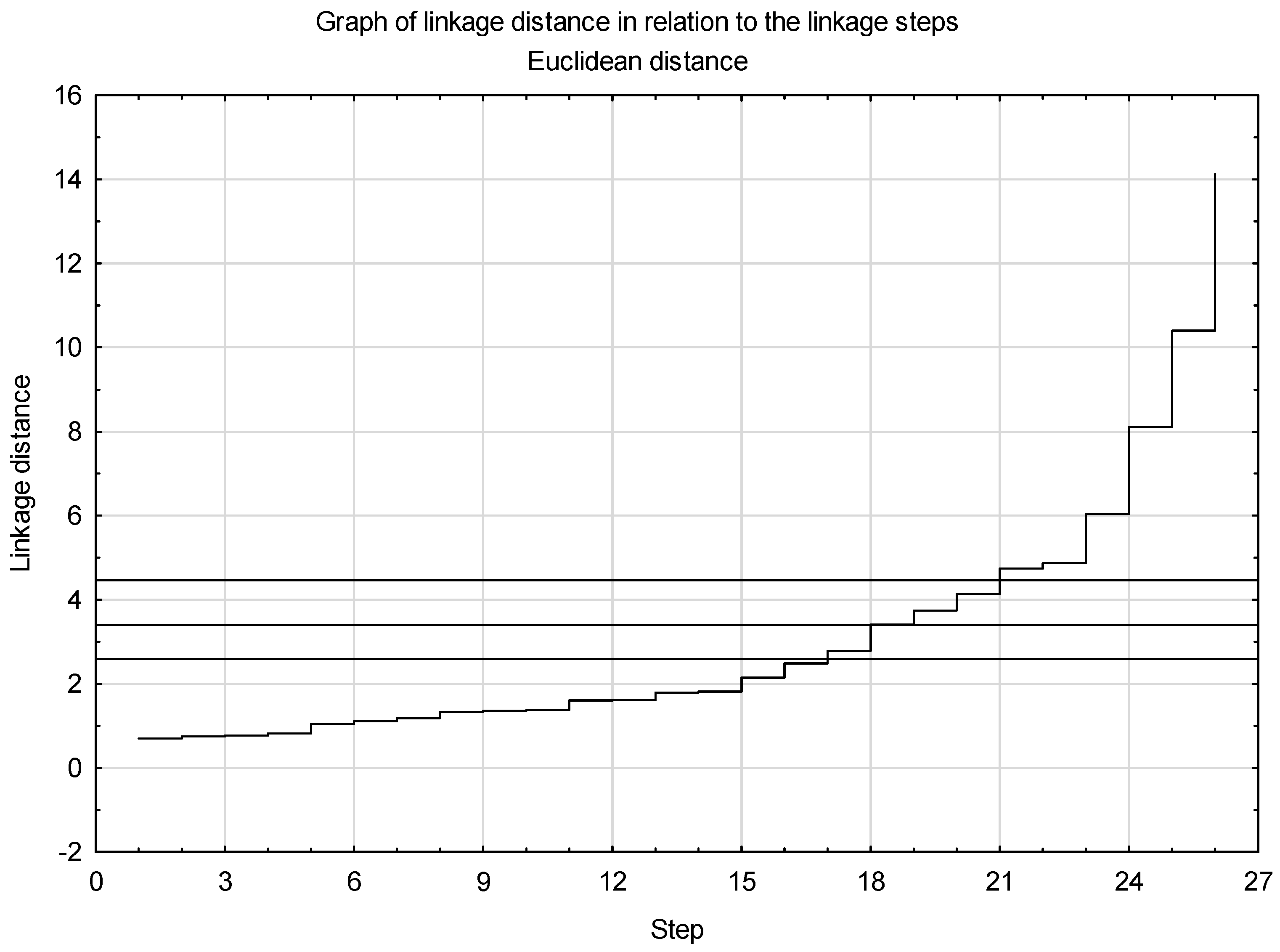
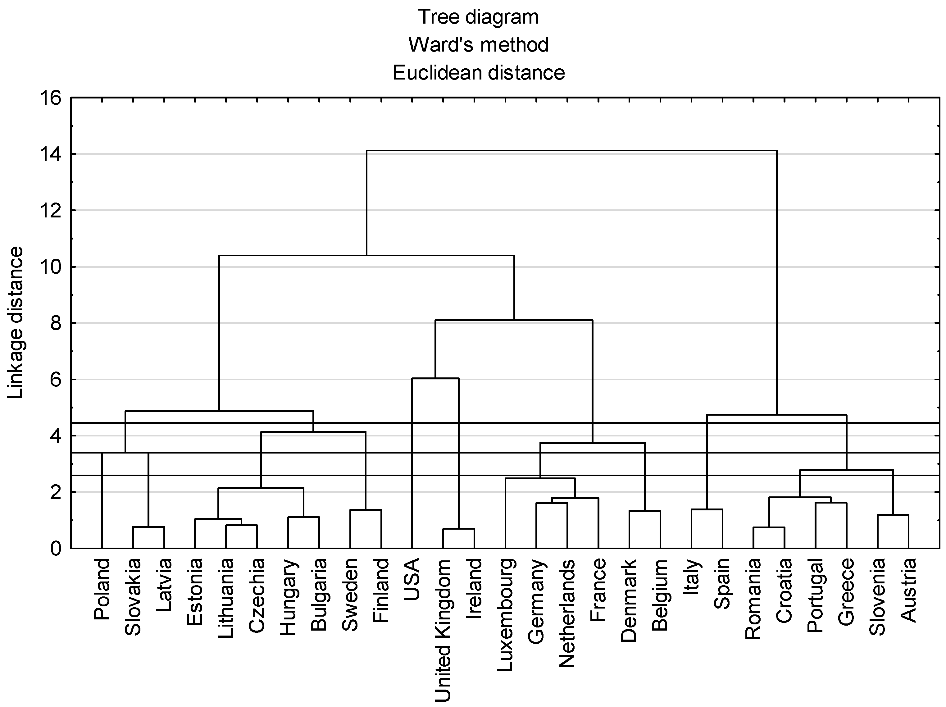
Section 2.2.2, three procedures of the tree-diagram division were applied. The maximum difference in the distance measure and the Grabiński measure were 3.40 and 2.60, respectively, thus indicating the division of the tree-diagram between the 18th and 19th or the 17th and 18th steps (Figure 1) and leading to the isolation of 10 or 11 classes of analyzed countries (
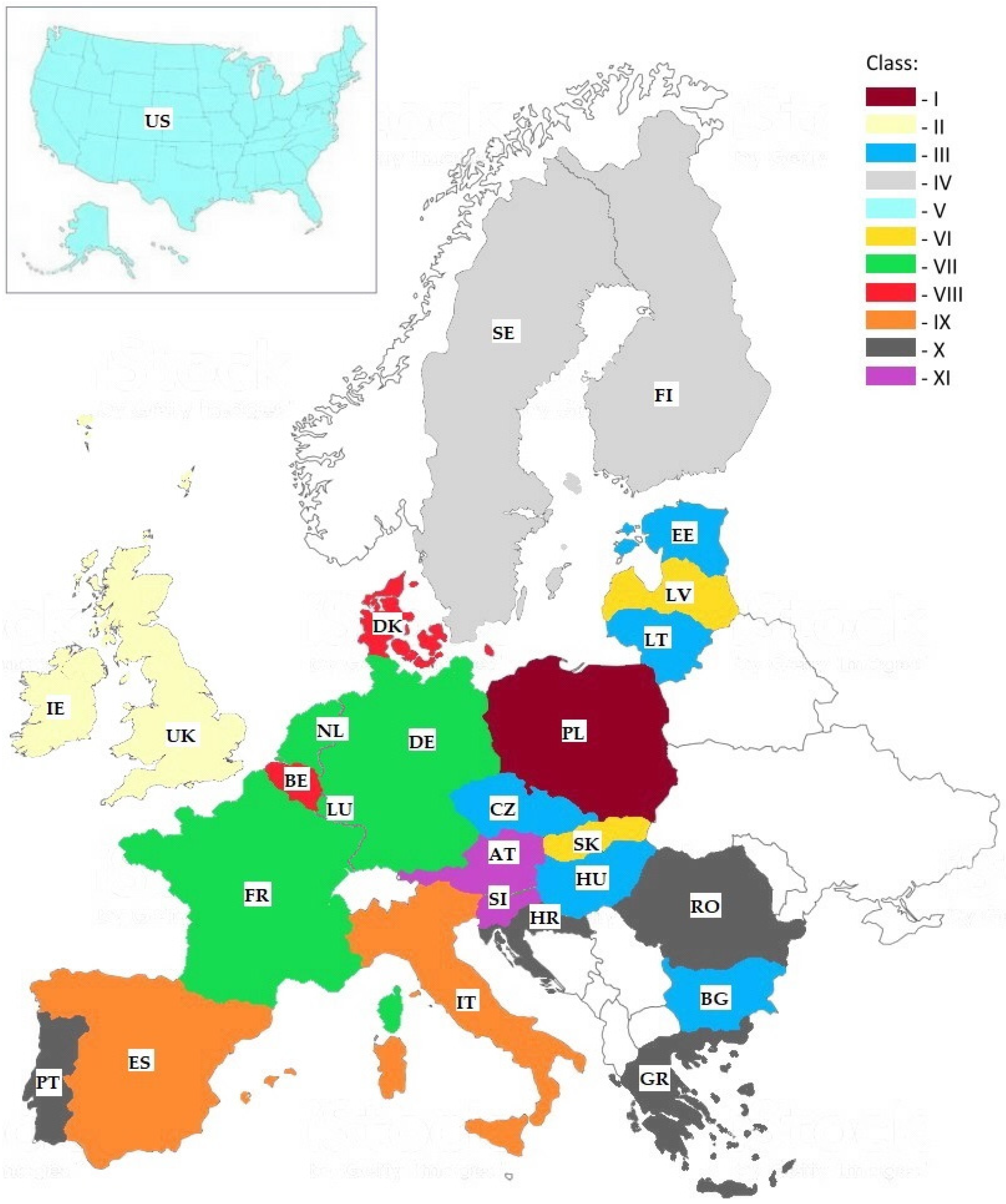
Figure 2). Applying the rule proposed by R. Mojena, for parameter k = 1.25 the value of 4.46 was obtained, which suggests the position of the tree-diagram division after the 21st step and thus distinguishes 7 classes of countries. Considering the division of the tree-diagram at the linkage distance determined by the value of the Grabiński measure as the most accurate, eleven classes of countries were distinguished as differing in the structure, intensity, and efficiency of utilization of their production potential in the agricultural sector (Figure 3). Values of class means for active characteristics are given in Table 4, while Table 5 gives values of the measure of differences between mean metrics, used to identify features characteristic to individual classes. Table 6 presents characteristics of typological classes of the analyzed countries depending on the production potential of their agricultural sector.
Class 1 includes Poland, characterized by a high share of labor in total inputs—the highest in the investigated population of countries—at the simultaneous low UAA per 1 person employed in agriculture (Figure 3, Table 5 and Table 6). A lower level of land assets for the labor production factor was recorded only in class 10 (Table 4), composed of Croatia, Portugal and Greece, having much lower resources of land than Poland as well as Romania, in which 300 thousand people employed more worked on almost 2 million ha smaller total UAA than in Poland (Table 1). It may be stated that due to the considerable resources of land and labor accumulated in Polish and Romanian agriculture their production potential is considerable in relation to the agriculture of the EU-28, and in terms of labor resources labor even compared to the USA. Nevertheless, it needs to be remembered that both land and labor resources are “potentially dormant”, which under advantageous external conditions may be effectively used, while under adverse conditions they will be a burden and will hinder development. The fragmented agrarian structure in those countries (see e.g., [30,87,93,94]), while not necessarily determining their production potential [95], will nevertheless have a considerable impact and will negatively affect the level of labor productivity, thus influencing also the level and accumulation of income. In turn, a factor stimulating income of farms in Poland may be provided by the very high ratio of current assets to fixed assets—by 75% exceeding the average for all the investigated countries (Table 4). A high ratio of current assets to fixed assets, by 50% exceeding the average for the analyzed population, was also recorded for Slovakia and Latvia constituting class 2 (Figure 3, Table 4). Importance of respective ratios between production factors modifying the financial situation of farms in the EU countries was already shown by Poczta et al. [96]. They indicated that good levels of production factors, at their inappropriate ratios, do not guarantee advantageous financial effects, whereas smaller economic entities, but this time with more appropriate ratios between the production factors, may attain satisfactory values of financial indexes.
Class 3, which includes five EU-13 countries—Estonia, Lithuania, Czechia, Hungary, and Bulgaria, showed no particularly characteristic features compared to the other countries (Figure 3, Table 5 and Table 6). When comparing this class to the entire investigated population we may observe the ratio of current assets to fixed assets and the productivity of current assets almost equal to the average, as well as lower assets of land and capital available to labor assets and average values of the other characteristics (Table 4).
Class 4 comprises two Scandinavian countries—Sweden and Finland, in which the share of land in total inputs was 2-fold lower than the average for all the investigated countries, as well as the lowest productivity of current assets in the analyzed population (Figure 3, Table 4). The value of agricultural production obtained from 1 euro of current assets in those countries was 1.36 euro and 1.21 euro, respectively, and it was by approx. 20–30% lower than in the EU-28 and by 30–40% lower than in the USA (Table 3). However, it results from a study by Kijek et al. [40] that Sweden and Finland belonged to the EU-15 countries characterized by the strongest convergence processes of agricultural productivity.
Class 5 was composed of 1 element, the USA with a low share of labor in total inputs, but over 3.5-fold and 2-fold higher land and capital assets per 1 person employed compared to the average for the investigated population of countries (Figure 3, Table 4). The ratio of current assets to fixed assets in the USA was also by over 40% higher the average. As mentioned in Section 3.1, advantageous ratios between production factors and a much more concentrated agrarian structure [30] promoted high productivity of labor and capital in the US agriculture (Table 3). It should be noted here that in 2017 in the USA farms with an area exceeding 105 ha UAA accounted for almost 25% all farms, but used almost 90% total UAA, while in the EU-28 less than 3% farms larger than 100 ha UAA concentrated almost 53% resources of agricultural land [30]. This is corresponding to the study by Huffmann and Evenson [97], who found that the structural change in the US agriculture related to farm size and specialization is an important source of total factor productivity growth both in crop and livestock production.
Class 6 included the United Kingdom and Ireland (Figure 3), characterized by much higher share of land in total inputs than in the other classes (Table 4, Table 5 and Table 6) as well as the highest UAA per 1 person employed in the EU-28 (Table 2). It needs to be stressed here that approx. 63% total UAA in the United Kingdom and as much as 90% in Ireland were permanent grasslands used in extensive cattle rearing based on grazing [58], which was reflected in land productivity by approx. 30% and 40% lower than the mean in the EU-28 and EU-15 (Table 3).
Class 7 comprised Luxembourg, Germany, the Netherlands and France, while class 8 included Denmark and Belgium (Figure 3) belonging to the group of most developed EU countries in terms of their GDP per capita measured in the purchasing power parity [98]. Those countries incurred the highest capital inputs per 1 ha UAA and per 1 employed in the EU-28 (Table 2), which contributed to the above-average productivity of land and labor within the EU-28 (Table 3). The high agricultural productivity of the above-mentioned countries was also indicated by Cuerva [99], Baer-Nawrocka and Markiewicz [22], Nowak and Różańska-Boczula [36], or Smędzik et al. [41]. In view of the high level of capital assets per 1 person employed and the recorded level of labor productivity, those two classes of countries are likely to include those capable of meeting the competitive pressure exerted by the more concentrated US agriculture, benefitting from the appropriate ratios of production factors, and being more productive as a result.
Class 9 comprises Italy and Spain, in comparison to the other countries distinguished by the ratio of current assets to fixed assets being by 40% lower, at a 20% higher productivity of current assets (Figure 3, Table 4, Table 5 and Table 6). The level of capital inputs per 1 person employed in those countries was relatively low, which was connected with the specialization in plant production (fruit and vegetables, olives, vineyards), being more land- and labor-intensive rather than capital-intensive. The other EU countries of the Mediterranean region (Croatia, Portugal, and Greece) as well as Romania, similarly as countries from class 9 specializing in plant production, were assigned to class 10 (Figure 3). In the investigated population they were distinguished by a low share of land, but a high share of labor in total inputs, comparable to that observed in in Poland and by over 30% higher than the mean for all the analyzed countries (Table 4 and Table 5). As was already mentioned, a relatively small UAA or excessive level of employment in in agriculture in relation to the available resources of agricultural land (Table 1) resulted in this class in the lowest level of land assets per 1 person employed. Fragmentation of farms as well as high labor intensity and lower capital intensity of production in countries of Southern Europe, related with the production structure to a considerable extent focused on plant production promoted by the advantageous climatic conditions was indicated by Baer-Nawrocka and Markiewicz [22].
Labor-intensive production of fruits, grapes and olives is also run in Slovenia, which together with Austria, being a leading organic producers in the EU [100,101], was classified to class 11 (Figure 3). For this class, similarly as for classes 1 and 10, a typical characteristic was the high share of labor in total inputs (Table 5 and Table 6), whereas in contrast to them in Austria and Slovenia a low ratio of current assets to fixed assets was recorded (Table 4), determining productivity of production factors lower than the EU-28 average (Table 3).

4. Conclusions

Although the EU and the US are the largest players in the global agricultural market and major trade partners for each other, there are only a few comparative studies concerning their agricultural potential and performance. No comprehensive study covering all individual EU member states in relation to the USA has been delivered so far. Considering the above and in view of the lasting impasse in the negotiations on both international and transatlantic trade liberalization, differences in the production structures seem to be a decisive factor affecting the competitiveness of the EU and the US agriculture, the paper aims at determining the spatial diversity of agricultural potential and its productivity across the countries under investigation. The study attempts to answer the questions: What is the gap in the agricultural potential between individual EU countries and the USA? Which EU countries are able to face the competitive pressure exerted by the US agricultural producers and which ones lose this ability?
Based on the conducted analyses it may be stated that more appropriate ratios between production factors, and as a result higher efficiency of their utilization are found in the US agriculture, in which in 2017 the level of land and capital assets per 1 person employed was 9- and 3-fold higher, respectively, than in the EU-28. Such land-to-labor and capital-to-labor ratios resulted in an over 3.5-fold advantage of the USA in terms of labor productivity. In contrast, the inferior capital-to-land ratio made land productivity in the US agriculture more than 2-fold lower compared to that in the EU-28. However, it needs to be emphasized here that the extensive character of agricultural production in the USA comes from farmers’ decision tending to adopt cheaper and environmentally friendly production through lower capital intensity of production, while a comparable type of farming in some CEEC is a necessity resulting from the deficit of capital. Nevertheless, such an ecologically desirable production type is in line with the paradigm of sustainable agriculture, which is of high priority when setting the objectives for agricultural policies both in the EU and the USA. Considering the relatively small cross-country disproportions in terms of capital productivity, it may also be concluded that enhancing labor productivity can be of higher importance to the agricultural productivity than an increase in capital productivity. This deserves special attention in countries with abundant labor resources and a fragmented agrarian structure, where simultaneous land concentration processes and rationalization of employment are required. It is crucial for the improvement both in agricultural productivity and incomes on a microscale. Increasing the level of agricultural productivity seems to be particularly decisive to the competitive position of those EU-13 countries, which so far have gained from cost and price advantages. Plentiful labor resources resulting in low wages do not secure a steady and resilient competitive advantage over the more productive countries. Moreover, considering the processes of price convergence in the EU countries posing a risk of an almost complete loss of the cost advantage, improving the ratios between production factors and boosting the efficiency of their use is more and more vital to enhance the competitive capacity of the agricultural sector in this group of countries.
It results from the conducted typological analysis that only among such countries as Germany, the Netherlands, France, Denmark, and Belgium we may find those capable of meeting the competitive pressure exerted by the more concentrated US agriculture, benefitting from the proper ratios between production factors. A much more difficult competitive situation is observed in the EU countries from Central and Eastern Europe as well as the Mediterranean, specializing in land- and labor-intensive production, requiring no major inputs of fixed capital. Even is some countries from those regions generated a considerable production potential manifested in the resources of land and labor (e.g., Poland and Romania), its rational utilization is hindered by structural deficits, resulting from the fragmented agrarian structure and low levels of land and capital assets per 1 person employed. In this context, in order to improve competitiveness of the agricultural sector the EU countries from Central and Eastern Europe and from Southern Europe have to improve the ratios of production factors. This may be stimulated by the institutional support for the concentration of the agrarian structure and policies focusing on technical change and innovation. In the case of countries with excessive employment in agriculture a key issue is to reduce employment levels, which will make it possible to increase the productivity of labor and the level of income from farms, as a result promoting modernization of farms and leading to desirable, environmentally friendly production. Since the process leading to reduced employment in agriculture to a considerable extent depends on the opportunities to find employment outside agriculture, the structural transformation may be supported by the properly designed labor market policy facilitating inter-sectoral labor flows and increasing off-farm labor market participation.
Considering that both the EU and the US strongly support their agricultural sectors, it may be of interest to revise the research results and measure agricultural productivity using agricultural output increased by government payments. Calculating total factor productivity instead of partial productivities and employing those values in the agglomerative procedure would also be valuable in the course of further research. Finally, a long-run analysis of changes in the production structures and their efficiency would deliver interesting findings. It would help to answer the question whether the distance between these two serious competitors in the world agricultural market (and between individual EU countries and the US) converged or diverged over last decades.

Author Contributions

Conceptualization, K.P., L.S., and P.K.; methodology, K.P.; formal analysis, K.P.; investigation, K.P.; resources, K.P.; writing—original draft preparation, K.P., L.S., and P.K.; writing—review and editing, K.P., L.S., and P.K.; visualization, K.P.; supervision, K.P.; project administration, K.P.; funding acquisition, K.P. All authors have read and agreed to the published version of the manuscript.

Funding

This research was funded by the National Science Centre within the OPUS research project No. 2015/17/B/HS4/00262, titled “Polish agri-food sector under the implementation of the Transatlantic Trade and Investment Partnership agreement (TTIP)”. The APC was funded by the Faculty of Economics, Poznan University of Life Sciences.

Conflicts of Interest

The authors declare no conflict of interest.

References

  1. Porter, M.E. The Competitive Advantage of Nations; The Free Press: New York, NY, USA, 1990. [Google Scholar]
  2. Van Duren, E.; Martin, L.; Westgren, R. Assessing the Competitiveness of Canada’s Agrifood Industry. Can. J. Agric. Econ. 1991, 39, 727–738. [Google Scholar] [CrossRef]
  3. Van Duren, E.; Martin, L.; Westgren, R. A Framework for Assessing National Competitiveness and the Role of Private Strategy and Public Policy. In Competitiveness in International Food Markets; Bredahl, M.E., Abbott, P.C., Reed, M.R., Eds.; Westview Press: Boulder, CO, USA, 1994; pp. 37–59. [Google Scholar]
  4. Reiljan, J.; Hinrikus, M.; Ivanov, A. Key Issues in Defining and Analysing the Competitiveness of a Country; University of Tartu Economics and Business Administration Working Paper No. 1; Tartu University Press: Tartu, Estonia, 2000; Available online: https://papers.ssrn.com/sol3/papers.cfm?abstract_id=418540 (accessed on 7 February 2021).
  5. Kunasz, M. Zasoby przedsiębiorstwa w teorii ekonomii (Enterprise Resources from the Perspective of Economic Theory). Gospod. Nar. 2006, 10, 33–48. [Google Scholar] [CrossRef]
  6. Guth, M.; Smędzik-Ambroży, K. Economic resources versus the efficiency of different types of agricultural production in regions of the European Union. Econ. Res. Ekon. Istraživanja 2020, 33, 1036–1051. [Google Scholar] [CrossRef] [Green Version]
  7. Schumpeter, J.A. The Theory of Economic Development: An. Inquiry into Profits, Capital, Credit, Interest and the Business Cycle. Harvard Economic Studies, 46; Harvard University Press: Cambridge, MA, USA, 1936. [Google Scholar]
  8. Schumpeter, J.A. Business Cycles: A Theoretical, Historical and Statistical Analysis of the Capitalist Process; McGraw-Hill Book Company: New York, NY, USA, 1939; Volume 1. [Google Scholar]
  9. Tinbergen, J. Zur Theorie der langfristigen Wirtschaftsentwicklung (On the Theory of Long-Term Economic Development). Weltwirtschaftliches Arch. 1942, 55, 511–549. [Google Scholar]
  10. Solow, R.M. Technical Change and the Aggregate Production Function. Rev. Econ. Stat. 1957, 39, 312–320. [Google Scholar] [CrossRef] [Green Version]
  11. Fagerberg, J. A technology gap approach to why growth rates differ. Res. Policy 1987, 16, 87–99. [Google Scholar] [CrossRef]
  12. Fagerberg, J. International competitiveness. Econ. J. 1988, 98, 355–374. [Google Scholar] [CrossRef]
  13. Dunning, J.H. The Global Economy, Domestic Governance, Strategies and Transnational Corporations: Interactions and Policy Implications. Transnatl. Corp. 1992, 1, 7–45. [Google Scholar]
  14. Hämäläinen, T.J. National Competitiveness and Economic Growth. The Changing Determinants of Economic Performance in the World Economy; Edward Elgar Publishing Ltd.: Cheltenham, UK, 2003. [Google Scholar]
  15. Cho, D.-S.; Moon, H.-C. From Adam Smith to Michael Porter: Evolution of Competitiveness Theory; World Scientific: Singapore, 2000. [Google Scholar]
  16. Cho, D.-S.; Moon, H.-C. National competitiveness: Implications for Different Groups and Strategies. Int. J. Glob. Bus. Compet. 2005, 1, 1–11. [Google Scholar]
  17. Schultz, T.W. Transforming Traditional Agriculture; Yale University Press: New Haven, CO, USA, 1964. [Google Scholar]
  18. Brinkman, G.L. The Competitive Position of Canadian Agriculture. Can. J. Agric. Econ. 1987, 35, 263–288. [Google Scholar] [CrossRef]
  19. Abbott, P.C.; Bredahl, M.E. Competitiveness: Definitions, Useful Concepts and Issues. In Competitiveness in International Food Markets; Bredahl, M.E., Abbott, P.C., Reed, M.R., Eds.; Westview Press: Boulder, CO, USA, 1994; pp. 11–35. [Google Scholar]
  20. Ahearn, M.; Yee, J.; Ball, E.; Nehring, R.; Somwaru, A.; Evans, R. Agricultural Productivity in the U.S.; Agriculture Information Bulletin No. 740; Resource Economics Division, Economic Research Service, U.S. Department of Agriculture: Washington, DC, USA, January 1998.
  21. Latruffe, L. Competitiveness, Productivity and Efficiency in the Agricultural and Agri-Food Sectors; OECD Food, Agriculture and Fisheries Papers, No. 30; OECD Publishing: Paris, France, 2010. [Google Scholar] [CrossRef]
  22. Baer-Nawrocka, A.; Markiewicz, N. Relacje między czynnikami produkcji a efektywność wytwarzania w rolnictwie Unii Europejskiej (Production potential and agricultural effectiveness in European Union countries). J. Agribus. Rural Dev. 2013, 3, 5–16. [Google Scholar]
  23. Shumway, R.; Fraumeni, B.; Fulginiti, L.E.; Samuels, J.; Stefanou, S. Measurement of U.S. Agricultural Productivity: A 2014 Review of Current Statistics and Proposals for Change; Faculty Publications: Agricultural Economics 136; University of Nebraska-Lincoln: Lincoln, NE, USA, 2015; Available online: http://digitalcommons.unl.edu/ageconfacpub/136?utm_source=digitalcommons.unl.edu%2Fageconfacpub%2F136&utm_medium=PDF&utm_campaign=PDFCoverPages (accessed on 7 February 2021).
  24. Wang, S.L.; Heisey, P.; Schimmelpfennig, D.; Ball, A. Agricultural Productivity Growth in the United States: Measurement, Trends, and Drivers; Economic Research Report 189; Economic Research Service, U.S. Department of Agriculture: Washington, DC, USA, July 2015.
  25. Rzeszutko, A.; Kita, K. Competitiveness of Polish agriculture compared to the agriculture of the selected EU countries under the CAP. Rural Areas Dev. 2018, 15, 57–70. [Google Scholar]
  26. Czyżewski, A.; Smędzik-Ambroży, K. Specialization and diversification of agricultural production in the light of sustainable development. J. Int. Stud. 2015, 8, 63–73. [Google Scholar] [CrossRef] [PubMed]
  27. Czyżewski, B.; Smędzik-Ambroży, K. The regional structure of the CAP subsidies and the factor productivity in agriculture in the EU 28. Agric. Econ. Czech. 2017, 63, 149–163. [Google Scholar] [CrossRef] [Green Version]
  28. Duesterhaus, R. The SWCS view: Sustainability’s promise. J. Soil Water Conserv. 1990, 45, 4. [Google Scholar]
  29. Prus, P. Sustainable farming production and its impact on the natural environment—Case study based on a selected group of farmers. In Proceedings of the 8th International Scientific Conference Rural Development 2017: Bioeconomy Challenges, Aleksandras Stulginskis University, Kaunas, Lithuania, 23–24 November 2017; pp. 1280–1285. [Google Scholar] [CrossRef] [Green Version]
  30. Pawlak, K.; Poczta, W. Agricultural Resources and their Productivity: A Transatlantic Perspective. Eur. Res. Stud. J. 2020, 23, 18–49. [Google Scholar] [CrossRef]
  31. Marques, A.C.; Fuinhas, J.A.; Pais, D.F. Economic growth, sustainable development and food consumption: Evidence across different income groups of countries. J. Clean. Prod. 2018, 196, 245–258. [Google Scholar] [CrossRef]
  32. Carlisle, L.; de Montenegro Wit, M.; DeLonge, M.S.; Calo, A.; Getz, C.; Ory, J.; Munden-Dixon, K.; Galt, R.; Melone, B.; Knox, R.; et al. Securing the future of US agriculture: The case for investing in new entry sustainable farmers. Elem. Sci. Anthr. 2019, 7, 17. [Google Scholar] [CrossRef] [Green Version]
  33. Pawlak, K.; Kołodziejczak, M. The Role of Agriculture in Ensuring Food Security in Developing Countries: Considerations in the Context of the Problem of Sustainable Food Production. Sustainability 2020, 12, 5488. [Google Scholar] [CrossRef]
  34. Eurostat. Income and Living Conditions. Available online: https://ec.europa.eu/eurostat/web/main/data/database (accessed on 7 February 2021).
  35. Semega, J.; Kollar, M.; Shrider, E.A.; Creamer, J.F. Income and Poverty in the United States: 2019; U.S. Census Bureau, Current Population Reports P60-270; U.S. Government Publishing Office: Washington, DC, USA, 2020.
  36. Nowak, A.; Różańska-Boczula, M. Differentiation in the production potential and efficiency of farms in the member states of the European Union. Agric. Econ. Czech. 2019, 65, 395–403. [Google Scholar] [CrossRef]
  37. Tłuczak, A. Diversity of the selected elements of agricultural potential in the European Union countries. Agric. Econ. Czech. 2020, 66, 260–268. [Google Scholar] [CrossRef]
  38. Smędzik-Ambroży, K.; Sapa, A. Efficiency and technical progress in agricultural productivity in the European Union. Res. Pap. Wrocław Univ. Econ. 2019, 63, 115–126. [Google Scholar] [CrossRef]
  39. Baráth, L.; Fertö, I. Productivity and Convergence in European Agriculture. J. Agric. Econ. 2017, 68, 228–248. [Google Scholar] [CrossRef] [Green Version]
  40. Kijek, A.; Kijek, T.; Nowak, A.; Skrzypek, A. Productivity and its convergence in agriculture in new and old European Union member states. Agric. Econ. Czech. 2019, 65, 1–9. [Google Scholar] [CrossRef]
  41. Smędzik-Ambroży, K.; Rutkowska, M.; Hakan, K. Productivity of the Polish agricultural sector compared to European Union member states in 2004-2017 based on FADN farms. Ann. Paaae 2019, 21, 422–431. [Google Scholar] [CrossRef]
  42. Hamulczuk, M. Total factor productivity convergence in the EU agriculture. In International Conference on Competitiveness of Agro-Food and Environmental Economy Proceedings; The Bucharest University of Economic Studies: Bucharest, Romania, 2015; Volume 4, pp. 34–43. [Google Scholar]
  43. Alston, J.M.; Andersen, M.A.; Pardey, P.G. The Rise and Fall of U.S. Farm. Productivity Growth, 1910–2007; Staff Paper P15-02; University of Minnesota, College of Food, Agricultural and Natural Resource Sciences, Department of Applied Economics: St. Paul, MN, USA, January 2015. [Google Scholar]
  44. Griliches, Z. Research Expenditures, Education, and the Aggregate Agricultural Production Function. Am. Econ. Rev. 1964, 54, 961–974. [Google Scholar]
  45. Fuglie, K.O.; Heisey, P.W. Economic Returns to Public Agricultural Research; Economic Brief 10; United States Department of Agriculture, Economic Research Service: Washington, DC, USA, September 2007. [Google Scholar]
  46. Alston, J.M. The Benefits from Agricultural Research and Development, Innovation, and Productivity Growth; Food, Agriculture and Fisheries Working Papers, No. 31; OECD Publishing: Paris, France, 2010. [Google Scholar] [CrossRef]
  47. Jin, Y.; Huffman, W.E. Measuring public agricultural research and extension and estimating their impacts on agricultural productivity: New insights from U.S. evidence. Agric. Econ. 2016, 47, 15–31. [Google Scholar] [CrossRef] [Green Version]
  48. Fuglie, K.; Clancy, M.; Heisey, P.; MacDonald, J. Research, Productivity, and Output Growth in U.S. Agriculture. J. Agric. Appl. Econ. 2017, 49, 514–554. [Google Scholar] [CrossRef] [Green Version]
  49. Bureau, J.-C.; Färe, R.; Grosskopf, S. A Comparison of Three Nonparametric Measures of Productivity Growth in European and United States Agriculture. J. Agric. Econ. 1995, 46, 309–326. [Google Scholar] [CrossRef]
  50. Gopinath, M.; Arnade, C.; Shane, M.; Roe, T. Agricultural competitiveness: The case of the United States and major EU countries. Agric. Econ. 1997, 16, 99–109. [Google Scholar] [CrossRef] [Green Version]
  51. USDA. U.S.-EU Food and Agriculture Comparisons; Agriculture and Trade Reports, WRS-04-04; Economic Research Service, U.S. Department of Agriculture: Washington, DC, USA, January 2004.
  52. Gandolfo, G. The Classical (Ricardo-Torrens) Theory of Comparative Costs. In International Economics; Springer: Berlin/Heidelberg, Germany, 1986; pp. 7–32. [Google Scholar]
  53. Eurostat. Extra-EU Trade in Agricultural Goods. Available online: https://ec.europa.eu/eurostat/statistics-explained/index.php/Extra-EU_trade_in_agricultural_goods#Main_trading_partners_for_agricultural_products (accessed on 12 March 2021).
  54. Davidova, S.; Gorton, M.; Iraizoz, B.; Ratinger, T. Variations in Farm Performance in Transitional Economies: Evidence from the Czech Republic. J. Agric. Econ. 2003, 54, 227–245. [Google Scholar] [CrossRef]
  55. Baer-Nawrocka, A.; Markiewicz, N. Zróżnicowanie przestrzenne potencjału produkcyjnego rolnictwa w krajach Unii Europejskiej (The Spatial Differentiation of Agricultural Potential in EU Countries). Rocz. Nauk Rol. Ser. G 2010, 97, 9–15. [Google Scholar]
  56. Łukiewska, K.; Chrobocińska, K. Przestrzenne zróżnicowanie potencjału produkcyjnego rolnictwa w Polsce (Spatial Differentiation of Production Potential of Agriculture in Poland). Rocz. Nauk. Ekon. Rol. I Rozw. Obsz. Wiej. 2015, 102, 56–65. [Google Scholar]
  57. Poczta, W.; Średzińska, J.; Chenczke, M. Economic Situation of Dairy Farms in Identified Clusters of European Union Countries. Agriculture 2020, 10, 92. [Google Scholar] [CrossRef] [Green Version]
  58. Eurostat. Farm Structure. Available online: https://ec.europa.eu/eurostat/web/main/data/database (accessed on 30 January 2021).
  59. Eurostat. Economic Accounts for Agriculture. Available online: https://ec.europa.eu/eurostat/web/main/data/database (accessed on 30 January 2021).
  60. Eurostat. Land Prices and Rents. Available online: https://ec.europa.eu/eurostat/web/main/data/database (accessed on 31 January 2021).
  61. Eurostat. Labour Costs. Available online: https://ec.europa.eu/eurostat/web/main/data/database (accessed on 31 January 2021).
  62. USDA. Census of Agriculture 2017; United States Department of Agriculture, National Agricultural Statistics Service: Washington, DC, USA, 2019.
  63. U.S. Bureau of Labor Statistics. Average Hourly Earnings of All Employees, Total Private [CES0500000003]. Available online: https://fred.stlouisfed.org/series/CES0500000003 (accessed on 31 January 2021).
  64. Alvarez, S.; Paas, W.; Descheemaeker, K.; Tittonell, P.; Groot, J. Typology Construction, A Way of Dealing with Farm Diversity. General Guidelines for Humidtropics; Report for the CGIAR Research Program on Integrated System for the Humid Tropics; Wageningen University: Wageningen, The Netherlands, 2014. [Google Scholar]
  65. Blazy, J.-M.; Ozier-Lafontaine, H.; Doré, T.; Thomas, A.; Wery, J. A methodological framework that accounts for farm diversity in the prototyping of crop management systems. Application to banana-based systems in Guadeloupe. Agric. Syst. 2009, 101, 30–41. [Google Scholar] [CrossRef]
  66. Pacini, G.C.; Colucci, D.; Baudron, F.; Righi, E.; Corbeels, M.; Tittonell, P.; Stefanini, F.M. Combining Multi-Dimensional Scaling and Cluster Analysis to Describe the Diversity of Rural Households. Exp. Agric. 2014, 50, 376–397. [Google Scholar] [CrossRef] [Green Version]
  67. Kamińska, A.; Nowak, A. Zastosowanie analizy skupień do badania zróżnicowania regionalnego potencjału produkcyjnego rolnictwa w Polsce (An application of cluster analysis to make a survey of regional productive potential differentiation in Polish agriculture). Rocz. Nauk. Stowarzyszenia Ekon. Rol. I Agrobiz. 2014, 16, 126–130. [Google Scholar]
  68. Grabiński, T.; Sokołowski, A. The Effectiveness of Some Signal Identification Procedures. In Signal Processing: Theories and Applications; Kunt, M., De Coulon, F., Eds.; North-Holland Publishing Co.: Amsterdam, The Netherlands, 1980; pp. 617–623. [Google Scholar]
  69. Ward, J.H., Jr. Hierarchical Grouping to Optimize an Objective Function. J. Am. Stat. Assoc. 1963, 58, 236–244. [Google Scholar] [CrossRef]
  70. Milligan, G.W.; Cooper, M.C. A study of standardization of variables in cluster analysis. J. Classif. 1988, 5, 181–204. [Google Scholar] [CrossRef]
  71. Jajuga, K.; Walesiak, M. Standardisation of data set under different measurement scales. In Classification and Information Processing at the Turn of the Millennium; Decker, R., Gaul, W., Eds.; Springer: Berlin/Heidelberg, Germany, 2000; pp. 105–112. [Google Scholar]
  72. Cymerman, J.; Cymerman, W. Zastosowanie analizy skupień do klasyfikacji województw według rozwoju rynków nieruchomości rolnych (The Application of Cluster Analysis to the Classification of Voivodships According to the Development of Agricultural Real Estate Markets). Świat Nieruchom. World Real Estate J. 2017, 101, 55–61. [Google Scholar]
  73. Zalewska, E. Zastosowanie analizy skupień i metody porządkowania liniowego w ocenie polskiego szkolnictwa wyższego (Application of Cluster Analysis and Linear Ordering in the Assessment of Polish Higher Education). Res. Pap. Wrocław Univ. Econ. 2017, 469, 234–242. [Google Scholar] [CrossRef] [Green Version]
  74. Mojena, R. Hierarchical grouping methods and stopping rules: An evaluation. Comput. J. 1977, 20, 359–363. [Google Scholar] [CrossRef] [Green Version]
  75. Milligan, G.W.; Cooper, M.C. An examination of procedures for determining the number of clusters in a data set. Psychometrika 1985, 50, 159–179. [Google Scholar] [CrossRef]
  76. Wysocki, F. Metody Taksonomiczne w Rozpoznawaniu Typów Ekonomicznych Rolnictwa i Obszarów Wiejskich (Taxonomic Methods to Identify Economic Types of Agriculture and Rural Areas); Poznan University of Life Sciences: Poznań, Poland, 2010. [Google Scholar]
  77. Poczta, W. Rolnictwo Polskie w Przededniu Integracji z Unią Europejską (Polish Agriculture on the Eve of Integration with the European Union); Poznan University of Life Sciences: Poznań, Poland, 2003. [Google Scholar]
  78. Huettel, S.; Wildermann, L.; Croonenbroeck, C. How do institutional market players matter in farmland pricing? Land Use Policy 2016, 59, 154–167. [Google Scholar] [CrossRef]
  79. Seeman, T.; Šrédl, K.; Prášilová, M.; Svoboda, R. The Price of Farmland as a Factor in the Sustainable Development of Czeh Agriculture (A Case Study). Sustainability 2020, 12, 5622. [Google Scholar] [CrossRef]
  80. Martin-Retortillo, M.; Pinilla, V. Why did Agricultural Labour Productivity Not Converge in Europe from 1950 to 2005? EHES Working Paper No. 25; European Historical Economics Society: Paris, France, October 2012; Available online: http://www.ehes.org/EHES_No25.pdf (accessed on 14 February 2021).
  81. National Bank of Poland. Middle Exchange Rates Archive—Table A. Available online: https://www.nbp.pl/homen.aspx?c=/ascx/ArchAen.ascx (accessed on 30 January 2021).
  82. Debertin, D.L. Agricultural Production Economics, 2nd ed.; University of Kentucky: Lexington, KY, USA, 2012. [Google Scholar] [CrossRef]
  83. Tarnowska, A. Produktywność wybranych czynników wytwórczych w rolnictwie krajów Unii Europejskiej w latach 2005–2012 (Productivity of chosen production factors in agriculture in the European Union in the years 2005–2012). Rocz. Nauk. Stowarzyszenia Ekon. Rol. I Agrobiz. 2014, 16, 214–219. [Google Scholar]
  84. Pawlak, K.; Poczta, W. Competitiveness of Polish Agriculture in the Context of Globalization and Economic Integration Competitive Potential and Position. Probl. Agric. Econ. 2020, 4, 86–107. [Google Scholar] [CrossRef]
  85. Gołaś, Z. Labour Productivity Growth and Convergence in Agriculture of the European Union. Int. J. Econ. Financ. Issues 2019, 9, 11–17. [Google Scholar] [CrossRef]
  86. Nowak, A.; Krukowski, A. Competitiveness of farms in new European Union member states. Agron. Sci. 2019, 74, 73–80. [Google Scholar] [CrossRef]
  87. Burja, C.; Burja, V. Farms Size and Efficiency of the Production Factors in Romanian Agriculture. Econ. Agric. 2016, 63, 361–374. [Google Scholar]
  88. Bórawski, P.; Guth, M.; Bełdycka-Bórawska, A.; Jankowski, K.J.; Parzonko, A.; Dunn, J.W. Investments in Polish Agriculture: How Production Factors Shape Conditions for Environmental Protection? Sustainability 2020, 12, 8160. [Google Scholar] [CrossRef]
  89. Hornowski, A.; Parzonko, A.; Kotyza, P.; Kondraszuk, T.; Bórawski, P.; Smutka, L. Factors Determining the Development of Small Farms in Central and Eastern Poland. Sustainability 2020, 12, 5095. [Google Scholar] [CrossRef]
  90. Špička, J.; Smutka, L. The Technical Efficiency of Specialised Milk Farms: A Regional View. Sci. World J. 2014, 985149. [Google Scholar] [CrossRef] [PubMed] [Green Version]
  91. Latruffe, L.; Balcombe, K.; Davidova, S.; Zawalińska, K. Determinants of technical efficiency of crop and livestock farms in Poland. Appl. Econ. 2004, 36, 1255–1263. [Google Scholar] [CrossRef]
  92. Bojnec, S.; Latruffe, L. Farm. Size and Efficiency: The Case of Slovenia. In Proceedings of the 100th seminar of the EAAE, Development of Agriculture and Rural Areas in Central and Eastern Europe, Novi Sad, Serbia, 21–23 June 2007. [Google Scholar]
  93. Burja, V. Performance Disparities Between Agricultural Holdings of Romania and of the European Union. Ann. Constantin Brâncuşi Univ. Târgu Jiueconomy Ser. 2014, 97–102. [Google Scholar]
  94. Alexandri, C.; Gavrilescu, C.; Luca, L.; Voicilas, D.-M. National Strategy for Agriculture in Romania—Horizon 2035. Rural Areas Dev. 2017, 14, 135–152. [Google Scholar]
  95. Wiatrak, A.P. Dochody i Akumulacja w Gospodarce Chłopskiej (Income and Accumulation in the Peasant Economy); PWN Group: Warsaw, Poland, 1982. [Google Scholar]
  96. Poczta, W.; Średzińska, J.; Standar, A. Sytuacja finansowa gospodarstw rolnych krajów UE według potencjału produkcyjnego (Financial situation in the agricultural holdings of the EU countries according to the potential for production). J. Agribus. Rural Dev. 2008, 4, 83–94. [Google Scholar]
  97. Huffmann, W.E.; Evenson, R.E. Structural and productivity change in US agriculture, 1950–1982. Agric. Econ. 2001, 24, 127–147. [Google Scholar] [CrossRef]
  98. Eurostat. National Accounts. Available online: https://ec.europa.eu/eurostat/web/main/data/database (accessed on 16 February 2021).
  99. Cuerva, M.C. Dynamics of European agricultural productivity: An analysis of regional convergence. Rev. Agric. Environ. Stud. 2011, 92, 237–258. [Google Scholar]
  100. Brückler, M.; Resl, T.; Reindl, A. Comparison of organic and conventional crop yields in Austria. Die Bodenkult. J. Land Manag. Food Environ. 2017, 68, 223–236. [Google Scholar] [CrossRef] [Green Version]
  101. Darnhofer, I.; D’Amico, S.; Fouilleux, E. A relational perspective on the dynamics of the organic sector in Austria, Italy, and France. J. Rural Stud. 2019, 68, 200–212. [Google Scholar] [CrossRef]
Figure 1. The course of agglomeration in the EU countries and the USA depending on the production potential of the agricultural sector. Source: The authors’ calculations based on [58,59,60,61,62,63].
Agriculture 11 00282 g001
Figure 2. Tree-diagram division of the EU countries and the USA depending on the production potential of the agricultural sector (Ward’s method, Euclidean distance). Note: Due to a lack of comprehensive data on land prices and wages making the calculation of the global inputs structure impossible Cyprus and Malta were excluded from the typological analysis. Source: The authors’ calculations based on [58,59,60,61,62,63].
Agriculture 11 00282 g002
Figure 3. Typology of the EU countries and the USA depending on the production potential of the agricultural sector (Ward’s method, Euclidean distance). Note: Austria (AT), Belgium (BE), Bulgaria (BG), Croatia (HR), Czechia (CZ), Denmark (DK), Estonia (EE), Finland (FI), France (FR), Germany (DE), Greece (GR), Hungary (HU), Ireland (IE), Italy (IT), Latvia (LV), Lithuania (LT), Luxembourg (LU), Netherlands (NL), Poland (PL), Portugal (PT), Romania (RO), Slovakia (SK), Slovenia (SI), Spain (ES), Sweden (SE), United Kingdom (UK), USA (US). Source: The authors’ calculations based on [58,59,60,61,62,63].
Agriculture 11 00282 g003
Table 1. Utilized agricultural area (UAA), labor inputs and capital inputs in the agriculture of the EU and the USA in 2017.
CountriesUAA aEmploymentCapital Input (Intermediate Consumption and Fixed Capital Consumption) b
Thous. ha%Thous. Persons%Million Euro%
Austria26701.5167.41.85831.31.9
Belgium13540.854.00.66785.32.2
Denmark26151.561.60.69443.93.1
Finland21941.392.91.04302.41.4
France27,81416.1697.97.453,726.217.7
Germany16,7159.7532.05.646,009.815.1
Greece45542.6453.44.86821.12.2
Ireland48842.8110.41.26167.22.0
Italy12,5987.3871.29.233,695.411.1
Luxembourg1310.13.10.0407.10.1
Netherlands17961.0176.01.921,061.66.9
Portugal36422.1304.43.25446.11.8
Spain23,23013.4819.48.626,983.68.9
Sweden30211.791.51.05611.11.8
United Kingdom16,3949.5369.63.921,359.27.0
EU-15123,61271.44804.850.7253,651.283.4
Bulgaria44922.6221.02.32735.10.9
Croatia15630.9113.31.21538.20.5
Cyprus1120.19.60.1416.80.1
Czechia34552.0146.31.54121.21.4
Estonia9950.623.10.2738.20.2
Hungary46712.7222.72.35794.91.9
Latvia19311.161.40.61108.10.4
Lithuania29251.7105.51.12237.90.7
Malta110.02.20.068.80.0
Poland14,4068.31672.217.616,758.05.5
Romania12,5037.21974.920.812,077.14.0
Slovakia18901.168.50.71976.20.6
Slovenia4880.353.00.6984.80.3
EU-1349,44228.64673.749.350,555.416.6
EU-28173,054100.09478.5100.0304,206.6100.0
USA364,305100.02188.2100.0206,048.8100.0
Note: a—data for EU countries for 2016; b—value of capital inputs in US agriculture converted from USD to EUR based on the mean annual exchange rate of NBP [81]. Source: The authors’ calculations based on [58,59,60,61,62,63].
Table 2. Ratios between production factors in the EU and US agriculture in 2017.
CountriesUAA per 1 Person Employed (ha)Value of Capital Inputs per 1 Person Employed (Thous. Euro)Value of Capital Inputs per 1 ha UAA (Thous. Euro)
Austria15.9534.832.18
Belgium25.07125.655.01
Denmark42.45153.313.61
Finland23.6246.311.96
France39.8576.981.93
Germany31.4286.482.75
Greece10.0415.041.50
Ireland44.2455.861.26
Italy14.4638.682.67
Luxembourg42.26131.323.11
Netherlands10.20119.6711.73
Portugal11.9617.891.50
Spain28.3532.931.16
Sweden33.0261.321.86
United Kingdom44.3657.791.30
EU-1525.7352.792.05
Bulgaria20.3312.380.61
Croatia13.8013.580.98
Cyprus11.6743.423.72
Czechia23.6228.171.19
Estonia43.0731.960.74
Hungary20.9726.021.24
Latvia31.4518.050.57
Lithuania27.7321.210.77
Malta5.0031.276.25
Poland8.6110.021.16
Romania6.336.120.97
Slovakia27.5928.851.05
Slovenia9.2118.582.02
EU-1310.5810.821.02
EU-2818.2632.091.76
USA166.4994.160.57
Source: The authors’ calculations based on [58,59,60,61,62,63].
Table 3. Productivity of production factors in the agriculture of the EU and the USA in 2017.
CountriesAgricultural Production
Per 1 ha UAAPer 1 Person EmployedPer 1 Euro of Capital InputsPer 1 Euro of Current Assets
EuroEU-28 = 100EuroEU-28 = 100EuroEU-28 = 100EuroEU-28 = 100
Austria2580106.941,14693.41.1886.01.6998.8
Belgium6167255.5154,622351.01.2389.61.3981.3
Denmark4210174.5178,708405.61.1784.91.3679.6
Finland171070.940,38591.70.8763.51.2170.6
France2555105.9101,842231.21.3296.41.6495.9
Germany3388140.4106,437241.61.2389.71.5892.6
Greece2415100.124,25755.11.61117.51.95114.0
Ireland173671.976,779174.31.37100.11.5993.2
Italy4025166.858,210132.11.51109.62.14125.4
Luxembourg3002124.4126,845287.90.9770.41.2874.5
Netherlands15,667649.3159,877362.91.3497.31.6495.7
Portugal204284.624,42755.41.3799.51.6093.4
Spain212988.260,348137.01.83133.52.27132.6
Sweden203184.267,054152.21.0979.71.3679.3
United Kingdom171871.276,203173.01.3296.11.5691.3
EU-152812116.572,345164.21.3799.81.73100.9
Bulgaria91237.818,53442.11.50109.11.79104.6
Croatia136956.718,87942.91.39101.31.74101.8
Cyprus6217257.672,527164.61.67121.71.73101.2
Czechia142359.033,60876.31.1986.91.4484.3
Estonia85235.336,70083.31.1583.71.3981.5
Hungary176473.137,00784.01.42103.61.7199.8
Latvia66827.721,00747.71.1684.81.3276.9
Lithuania95239.526,40659.91.2490.71.4785.7
Malta10,465433.752,327118.81.67121.91.84107.8
Poland177373.515,27734.71.52111.11.7099.4
Romania127152.7805018.31.3295.91.6898.2
Slovakia119949.733,09575.11.1583.61.3076.2
Slovenia236397.921,75549.41.1785.31.6093.3
EU-13141658.714,97634.01.38100.91.6495.9
EU-282413100.044,057100.01.37100.01.71100.0
USA94639.2157,535357.61.67121.91.91111.4
Source: The authors’ calculations based on [58,59,60,61,62,63].
Table 4. Mean intraclass features describing production potential of the agricultural sector in the EU countries and the USA.
FeatureClassTotal
IIIIIIIVVVIVIIVIIIIXXXI
Share of land in total inputs (%)1.21.31.20.82.73.51.31.81.61.01.91.9
Share of labor in total inputs (%)61.238.937.250.133.544.437.733.050.761.058.946.1
UAA per 1 person employed (ha)8.629.423.028.3166.544.333.034.321.27.814.346.1
Value of capital inputs per 1 person employed (Thous. Euro)10.023.721.753.894.257.386.0140.435.99.130.943.7
Ratio of current assets to fixed assets (Euro/Euro)8.77.45.03.37.15.63.96.63.04.32.45.0
Productivity of current assets (Euro/Euro)1.71.31.61.31.91.61.61.42.21.71.71.8
Source: The authors’ calculations based on [58,59,60,61,62,63].
Table 5. Values of the measure of differences for mean metrics describing the production potential of the agricultural sector in the population of analyzed countries and in classes (Ward’s method).
FeatureClass
IIIIIIIVVVIVIIVIIIIXXXI
Share of land in total inputs (%)−1.7−1.6−1.7−2.71.93.8−1.4−0.3−0.8−2.3−0.1
Share of labor in total inputs (%)2.6−1.2−1.50.7−2.1−0.3−1.4−2.20.82.52.2
UAA per 1 person employed (ha)−2.3−1.0−1.4−1.17.3−0.1−0.8−0.7−1.5−2.3−1.9
Value of capital inputs per 1 person employed (Thous. Euro)−1.5−0.9−0.90.42.20.61.84.2−0.3−1.5−0.6
Ratio of current assets to fixed assets (Euro/Euro)3.92.60.1−1.72.20.7−1.11.7−2.1−0.7−2.7
Productivity of current assets (Euro/Euro)−0.7−3.4−1.2−3.50.8−1.6−1.2−2.92.9−0.4−0.8
Note: Cells shaded in grey denote features characteristic to a given class. Source: The authors’ calculations based on [58,59,60,61,62,63].
Table 6. Characteristics of types of analyzed countries distinguished based on the production potential of the agricultural sector.
ClassCharacteristics of Type
IHigh—the highest in the analyzed population—the share of labor in total inputs; small UAA per 1 person employed; very high ratio of current assets to fixed assets
IIHigh ratio of current assets to fixed assets; very low productivity of current assets
IIIAverage type, not distinguished by any particularly characteristic features from the other countries
IVLow share of land in total inputs—the lowest among analyzed countries; very low productivity of current assets—the lowest in the analyzed population
VLow share of labor in total inputs; very high UAA per 1 person employed—the highest in the analyzed population; high level of capital assets per 1 person employed and high ratio of current assets to fixed assets
VIVery high share of land in total inputs—the highest in the analyzed population
VIIAverage type, not distinguished by any particularly characteristic features from the other countries
VIIILow share of labor in total inputs; very high level of capital assets per 1 person employed—the highest in the analyzed population; low productivity of current assets
IXLow ratio of current assets to fixed assets; high productivity of current assets—the highest in the analyzed population
XLow share of land, but high share of labor in total assets; lowest level of land assets per 1 person employed in the analyzed population
XIHigh share of labor in total inputs and low ratio of current assets to fixed assets
Note: In the description of type only these features were used, which based on the value of measure of differences in means were considered characteristic to a given type (see Table 5). Source: The authors’ elaboration based on Table 4 and Table 5.
Publisher’s Note: MDPI stays neutral with regard to jurisdictional claims in published maps and institutional affiliations.

