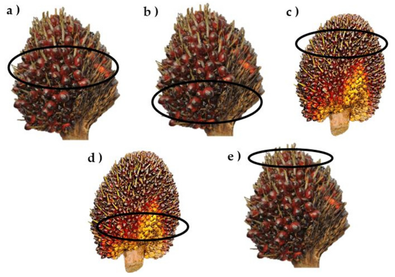
Application of Optical Spectrometer to Determine Maturity Level of Oil Palm Fresh Fruit Bunches Based on Analysis of the Front Equatorial, Front Basil, Back Equatorial, Back Basil and Apical Parts of the Oil Palm Bunches

Abstract

The quality of palm oil depends on the maturity level of the oil palm fresh fruit bunch (FFB). This research applied an optical spectrometer to collect the reflectance data of 96 FFB from unripe, ripe, and overripe classes for the maturity level classification. The spectrometer scanned the FFB from different parts, including apical, front equatorial, front basil, back equatorial, and back basil. Principal component analysis was carried out to extract principal components from the reflectance data of each of the parts. The extracted principal components were used in an ANOVA test, which found that the reflectance data of the front equatorial showed statistically significant differences between the three maturity groups. Then, the collected reflectance data was subjected to machine learning training and testing by using the K-Nearest Neighbor (KNN) and Support Vector Machine (SVM). The front equatorial achieved the highest accuracy, of 90.6%, by using SVM as classifiers; thus, it was proven to be the most optimal part of FFB that can be utilized for maturity classification. Next, the front equatorial dataset was divided into UV (180–400 nm), blue (450–490 nm), green (500–570 nm), red (630–700 nm), and NIR (800–1100 nm) regions for classification testing. The UV bands showed a 91.7% accuracy. After this, representative bands of 365, 460, 523, 590, 623, 660, 735, and 850 nm were extracted from the front equatorial dataset for further classification testing. The 660 nm band achieved an 89.6% accuracy using KNN as a classifier. Composite models were built from the representative bands. The combination of 365, 460, 735, and 850 nm had the highest accuracy in this research, which was 93.8% with the use of SVM. In conclusion, these research findings showed that the front equatorial has the better ability for maturity classification, whereas the composite model with only four bands has the best accuracy. These findings are useful to the industry for future oil palm FFB classification research.

1. Introduction

The most productive oil crop, oil palm, can meet the enormous and growing global demand for vegetable oils—expected to reach 240 million tons by 2050 [1]. Oil palm trees produce three to eight times more oil than any other oil crop [1]. To achieve the same amount of soybean or coconut oil, four to ten times more land is needed [2]. According to Oil World, the world production of major vegetable oils in 2018 was 200.8 million tons, with palm oil accounting for 73% of it [3]. By 2025, the worldwide market for palm oil is expected to reach 25.3 billion USD. Palm oil is the main ingredient in many daily supplies, including soaps, cosmetics, detergents, candles, food shortening, cooking oil, margarine, feedstock, and more [4]. The main production of palm oil is contributed by Indonesia and Malaysia [5], with both countries producing a combined 90% of palm oil in the world. Asia is the largest consumer of palm oil, with India, China, and Indonesia consuming 40% of all palm oil in the industry [5]. In Europe, the total palm oil import increased by 5% in 2019, and the Roundtable on Sustainable Palm Oil (RSPO) demanded the continent to import 100% of its certified sustainable palm oil (CSPO) by 2020 [6]. The report by the European Palm Oil Alliance (EPOA) showed that 86% of European palm oil import is sustainable, proving that European countries are working towards closing the gap to the 100% set by RSPO [7]. Thus, the palm oil industry is a promising market around the world.

The FFB commercial value is dependent on the appearance of the bunch and the quantity of the oil extracted from the bunch. Ripe bunches are more valuable than unripe bunches because they contain more oil and have lower free fatty acid (FFA) levels than overripe bunches [8]. Therefore, the FFB maturity grading is an essential task at the mill to ensure the extracted oil fulfills the business viability and quality standards required of the extracted oil.

The Malaysia Palm Oil Board (MPOB) grades FFB into 17 different classes; ripe, underripe, unripe, overripe, empty, rotten, long stalk, unfresh, old, dirty, small, pest-damaged, diseased, dura, loose fruit, stored, and wet. These classifications are based on the “MPOB Manual of Grading Oil Palm Fresh Fruit Bunches Third Edition (2015)” [9]. The details of each class are described in

Table 1. MPOB Manual of Grading Oil Palm Fresh Fruit Bunches Third Edition (2015) [9].

Bunch Classifications	Description
Ripe	Reddish orange color fruits, has at least 10 sockets of detached fruitlets and more than fifty percent (50%) of the fruit still attached to the bunch at the time of inspection at the mill.
Underripe	Reddish orange color fruits and has at least 10 sockets of detached fruitlets at the time of inspection at the mill.
Unripe	Purplish black color fruits and without any socket of detached fruitlets at the time of inspection at the mill.
Overripe	Darkish red color fruits and has more than fifty percent (50%) of detached fruitlets but with at least ten percent (10%) of the fruits still attached to the bunch at the time of inspection at the mill.
Empty	Bunch which has more than ninety percent (90%) of detached fruitlets at the time of inspection at the mill.
Rotten	Bunch partly or wholly, including its loose fruits, has turned blackish in color, as well as rotten and moldy.
Long stalk	Bunch which has s stalk of more than 5 cm in length (measured from the lowest level of the bunch stalk).
Unfresh	Bunch which has been harvested and left in the field for more than 48 h before being sent to the mill. The whole fruit, or part of it, together with its stalk, has dried out. Normally, this type of bunch is dry and blackish in color.
Old	Bunches that have been harvested and left long on the farm before being shipped to the factory. The fruit still attached on this bunch has been wrinkled and is colored brownish or black. The stalk has also been wrinkled and is soft and fibrous, with a blackish color. Many relay seeds fall out of the outer layer of the bunch.
Dirty	Bunch with more than half of its surface covered with mud, sand, or other dirt particles and mixed with stone or foreign matter.
Small	Bunch which has small fruits and weighs less than 2.3 kg.
Pest damaged	Bunch with more than thirty percent (30%) of its fruits damaged by pest attacks, such as rats, etc.
Diseased	Bunch which has more than fifty percent (50%) parthenocarpic fruits and is not normal in terms of its size or its density.
Dura	Shell thickness 2–8 mm; ratio of shell to fruit 25–50%; ratio of mesocarp to fruit 20–60%; ratio of kernel to fruit 4–20%.
Loose fruit	Fruit detached from a fresh bunch because of ripeness and reddish orange in color.
Stored	Unripe bunch that was stored or left long after harvest.
Wet	Consignment of FFB which has excessive free water.

. Throughout the years, different researchers from around the world have developed various approaches to assess fruit maturity levels. Some of these have been used for the inspection phase of the FFB quality, while others are better suited for lab level applications. The latter includes the destructive test method and the non-destructive method. Chauhan et al. [10] state that non-destructive methods (NDM) are more effective than conventional methods as NDM are mainly based on physical properties, which correlate well with certain quality factors of crops. Besides, NDM do not rupture the fruit tissue and can be used to assess the internal variables of fruits. These include applications of LiDAR scanning [11], optical-based sensors [12], computer and camera vision system [13], laser-based imaging system [14], handheld optical spectrometer [15], LED optical sensor [16], thermal imaging technique [17], and fruit battery [18].

Table 2. Summary of oil palm maturity classifications.

Ref.	Equipment	Data Type	Analysis Method	Accuracies/Discoveries
[11]	LiDAR scanning sensor	NIR 905 nm	Linear equation of reflectance percentage	Fruits with greater ripeness have lower reflectance intensity
[12]	Optical sensor	670 nm	Average voltage readings for each ripeness class	When there is less chlorophyll content inside the FFB, the amount of light absorbed also lessens
[13]	Digital camera	RGB images, HSI, normalized RGB	Canonical discriminant function	85% accuracy
[15]	Oil palm ripeness detector (OPRiD)	UV, VIS, NIR	Various ML algorithm	85.7% accuracy
[16]	Multiband optical sensor	615 to 940 nm, oil content correlation	Discriminant analysis, KNN	88.2% accuracy
[17]	FLIR E60 and FLIR T440 thermal imaging cameras	Emissivity of FFB	Thermal imaging temperature vs. emissivity	Rotten bunch emissivity 98%, higher than normal bunch
[18]	Fruit battery with charging	Load resistance voltage		Fruits with moisture content less than 44% and average load voltage, Vavg, between 20 to 30 mV are considered ripe fruits
[19]	GigE camera	Hue, Saturation, and Intensity (HSI)	Linear regression (LR) and ANN	LR: 45% accuracy ANN: 70% accuracy
[20]	Multi-parameter fluorescence sensor: Multiplex®3	Blue-to-Red Fluorescence Ratio (BRR-FRF)	Classification and regression tree (C&RT)	90% accuracy
[21]	Hyperspectral camera (SPECIM, ImSpector V 10)	560 nm, 680 nm, 740 nm, 910 nm	Euclidean distance	97.92% accuracy
[22]	Multiband sensor	570, 670, 750, 870 nm	Discriminant analysis	85% accuracy
[23]	Multi-parameter fluorescence sensor: Multiplex®3	Fluorescence (Flavonoids, anthocyanin)	Stochastic Gradient Boosting Trees model	87.7% accuracy
[24]	Canon Powershot A430 digital camera	RGB images	Neuro fuzzy logic	73.3% accuracy
[25]	Olympus E-520 digital camera	RGB images	Fuzzy logic	86.67% accuracy
[26]	Vivotek IP8332 Network Bullet Camera	HSI model	ANN and PCA	93.33% accuracy
[27]	Hyperspectral camera (Imperx IPX-2 M 30)	400–1000 nm	ANN	830 nm identified as best wavelength; 98.67% overall accuracy
[28]	CCD camera (QICAM Colour Fast 1394, QImaging, Surrey, BC, Canada) and laser diode 658 nm	RGB images and backscattering images	LDA, QDA	85% accuracy

gives a summary of the applications of different NDM to classify FFB maturity levels.

Shabdin et al. [19] studied the maturity classifications by using the Hue, Saturation, and Intensity (HSI) approach and extracting HSI from RGB images. ANN analysis showed a 70% accuracy with this approach. Hafiz et al. [20] scanned FFB from four categories of unripe, underripe, ripe, and overripe by using a handheld multi-parameter fluorescence sensor called Multiplex^®3. The Blue-to-Red Fluorescence Ratio (BRR_FRF) was used in their research. The value of the blue-green (BGF) emission signal was divided by the value of the far-red emission (FRF) signal to get this information. Both ratios used a UV (375 nm) light-emitting diode as a source of excitation, resulting in an overall accuracy of 89.7%. Color and hyperspectral images were applied by Junkwon et al. [21] to estimate the weight and maturity of oil palm. The results of hyperspectral images showed a better confidence level than RGB images, where the classification of maturity was easier and more accurate. The author concluded that hyperspectral images have a better potential than RGB images to classify oil palm maturity levels. To assess oil palm FFB maturity, Saeed et al. [22] tested a multi-band portable, active optical sensor system with four spectral bands of 570, 670, 750, and 870 nm. Using spectral reflectance data, Mahalanobis distance proved to be a reliable method for measuring FFB maturity, with an overall accuracy of 85%.

Dayaf [15] proposed the application of a handheld spectrometer to classify oil palm maturity levels using the Oil Palm Ripeness Detector (OPRiD). The device can radiate a spectrum from eight different LED modules, including UV, blue, green, amber, red, deep red, far-red, and near-infrared. OPRID is a device designed based on these technologies (measures reflected EMR in AU form) for determining the degree of maturity and the color differences of the sensed surfaces of oil palm bunches. The experiment using this device achieved 85.7% by using 590 and 660 nm as a composite model.

The classifiers used in this analysis are the Support Vector Machine (SVM) and the K-Nearest Neighbors (KNN) in MATLAB R2020a. SVM is a machine learning algorithm that uses nonlinear kernel functions to map input data into a high dimensional feature space to search for a separate hyperplane [29]. The hyperplane performs classifications onto the input data. KNN is a machine learning algorithm that can be used to solve classification and regression problems [30] and assumes there are feature similarities to predict the values of new data points. It assigns these based on their distances to the points in the training set.

SVM has been applied in different agricultural fields to discover, unravel, quantify, and understand data-intensive processes in agricultural operational environments [31]. Khan et al. [32] reviewed articles that applied machine learning algorithms to oil palm research and found that SVM is the most frequently used algorithm. This is due to the appropriateness of SVM for both regression and classification problems, as well as its reliability as a standard algorithm for performance benchmarking. In the study by Sengupta and Lee [33], SVM was used to identify the number of immature green citrus fruits under natural outdoor conditions. The SVM classifier achieved 80.4% of accuracy. Ramos et al. [34] developed computer vision to count the number of fruits on coffee trees automatically with the assistance of SVM. SVM achieved 87.83% of visibility percentage in ripe or overripe classes and 86.36% of visibility percentage in the semi-ripe class. The visibility percentage achieved in the unripe class was 81.39%. Chung et al. [35] also implemented SVM to detect Bakanae disease, a seedborne fungal disease in rice seedlings, for which they were able to produce 87.9% accuracy. Nooni et al. [36] compared the performance of SVM and the maximum likelihood classifier (MLC) to map oil palm plantations, where SVM proved to have higher accuracy, at 78.3%, than MLC, with 71.9% accuracy.

Other than SVM, KNN was also used in various studies of oil palm. Dayaf [15] obtained 88.7% of accuracy for classifying FFB maturity levels using KNN. However, they found that KNN performed less accurately than ANN. Zolfagharnassab [37] used KNN to classify FFB maturity by using a difference in FFB temperature and ambient temperature (ΔTemp), and 74.3% accuracy was achieved.

The varied wavelengths of energy generated by a light source are referred to as the light spectrum. Nanometers are the units of measurement for light (nm). A wavelength of light or a band of light energy is represented by each nanometer. The visible light spectrum ranges from 380 nm to 780 nm. Each distinct wavelength in the visible light spectrum corresponds to a certain color. We perceive different colors when the light of a given wavelength reaches the retina of the human eye. UV (ultraviolet) light has a wavelength of about 400 nm and is found in the electromagnetic spectrum between visible light and X-rays. Since it has a shorter wavelength and a higher frequency than the light our brain interprets as pictures, this electromagnetic radiation is not visible to the naked eye. Near-infrared (NIR) light is defined as light that has a wavenumber between 12,500 and 4000 cm⁻¹ (wavelengths from 800 to 2500 nm) [38].

Traditionally, FFBs were graded manually. Trained graders inspected the quality and maturity of FFBs. However, this method is subjective and inaccurate. Even for a skilled grader, manually classifying oil palm FFB into maturity categories is a tough and time-consuming process. Furthermore, human perceptions of color are frequently inconsistent, affected by physical and psychological factors [13]. The overripe and unripe FFB at the mills has contributed to the low quality of oil extraction. Due to these weaknesses, optimum crude oil production cannot be achieved; hence, some operation costs become a loss and burden to manufacturers [39].

The growth of small data collecting units has been rapid in recent years as they can cover data details for broad coverage, enhancing understanding of crop spatial and temporal variability [40]. Sensors with smaller dimensions, lower costs, and higher performance that can be deployed and integrated into production processes allow for more data and, ultimately, more information [41]. In the experiment conducted in [42], the Smart Engine (OtO Photonics, Inc., Hsinchu City, Taiwan) (SE) Series Spectrometer was used to collect the reflectance of FFB, with the scanning process focused only on the front equatorial of the FFB, while the classification made use of the pure reflectance of the FFB (180 to 1100 nm) as the input. The highest accuracy acquired was 90.6%. Next, the principal component (PC) was extracted from the PCA as the input, and the obtained accuracy was 73.2% in classifying the FFB maturity level. Thirdly, specific bands were selected to compute vegetation indices for classification, and the normalized difference vegetation index 2 (NDVI2) produced 84.4% accuracy in classifying the FFB maturity level. In that research [42], only SVM was used as the classifier.

To improve the performance of the experiment, we proposed a new experiment in this study that focused on the application of the same spectrometer to collect the reflectance data of the light spectrum of FFB and classify them into three categories based on maturity level, which were unripe, ripe, and overripe. These three categories are critical, as there is a pressing need to avoid the harvesting of unripe fruits to avoid low oil yield. We explored the use of different bands across the light spectrum to investigate the ability of each band to classify FFBs. The reflectance of various bands is a popular technique in the study of FFB maturity level classifications. However, FFB varies in size, and its growth condition on the tree leads to varying amounts of sunlight exposure on each part. Some parts face the tree and may be covered by leaves, while other parts face the sun and receive different amounts of sunlight for photosynthesis. This situation causes the different parts of the FFB to have different colors. Previous research may have acquired data indiscriminately between the parts covered by leaves during the growing stage of the FFBs. In the research presented in this paper, instead of focusing on just the front equatorial as done in [42], we investigated the research gap by dividing FFB into five different parts—apical, front equatorial, front basil, back equatorial, and back basil—for analysis. Each one was scanned and compared to discover the best part of the FFB for maturity classification. Machine learning algorithms, i.e., SVM and KNN, were applied for classification accuracy testing.

2. Materials and Methods

2.1. Sample Preparation

The experiment in this research was undertaken at a large local oil palm mill in Banting, Selangor, Malaysia. The FFBs were prepared by trained graders and classified into the three highly critical maturity categories of oil palm fresh fruit bunches, that is, unripe, ripe, and overripe. Each category contained at least 30 samples. The FFBs were cleaned by a brush to remove dirt and dried leaves from them.

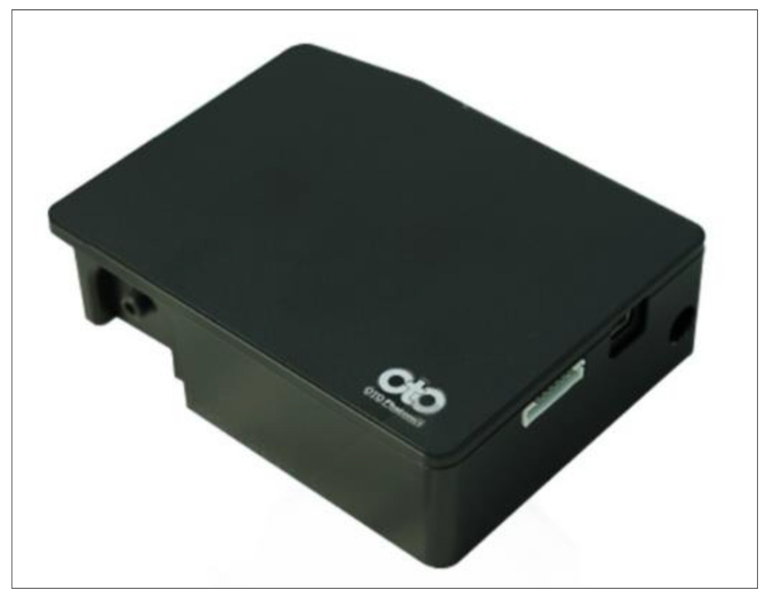
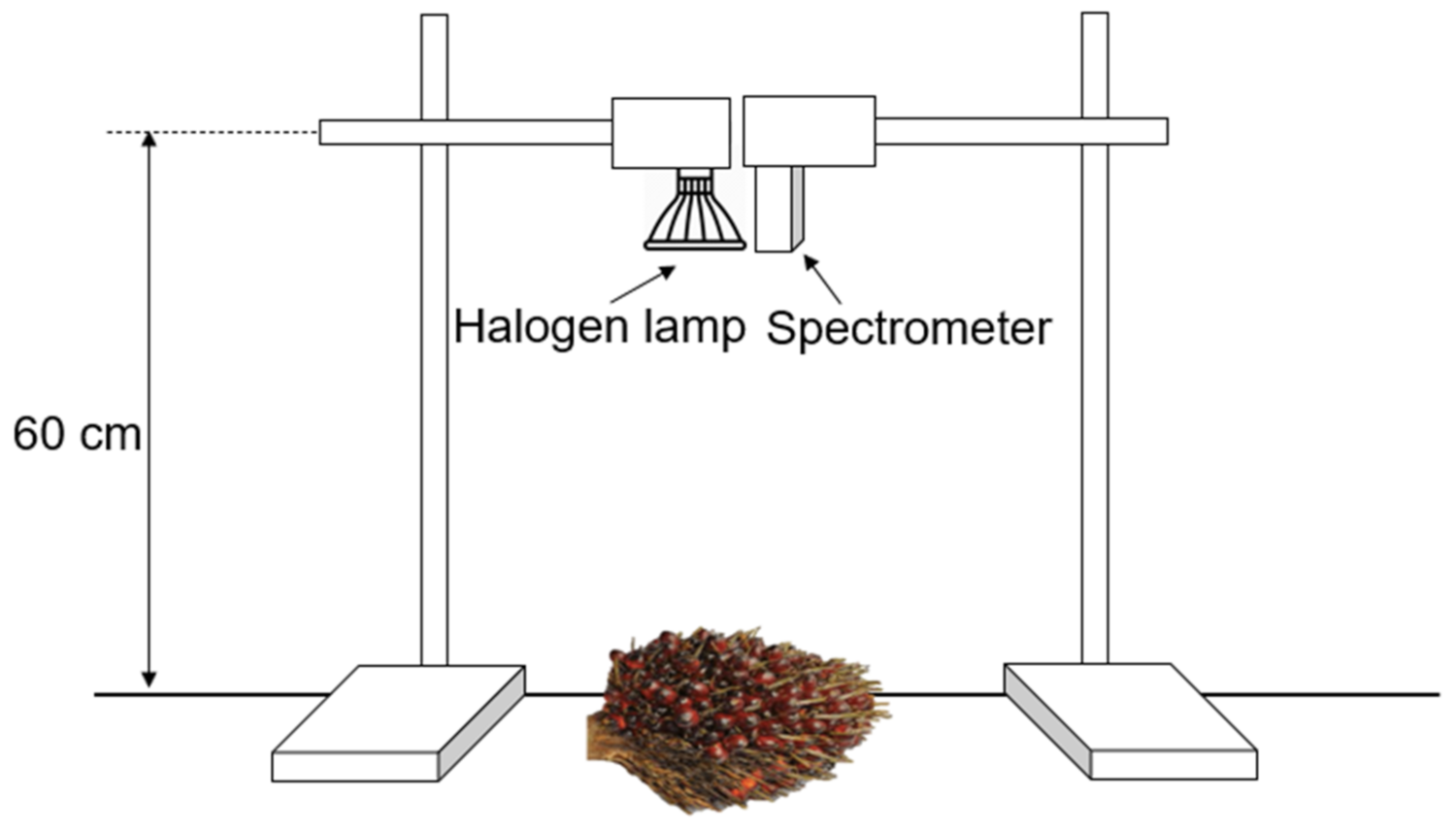
2.2. Data Collection

The device used was a SE Series spectrometer (OtO Photonics, Inc., Hsinchu City, Taiwan). The SE Series spectrometer is built with a linear CCD-type sensor and a high performance 32-bit RISC controller. The system is powered by USB port and communicates with computer through the USB port. The spectrometer has the ability to capture reflectance intensity at a wavelength range of 180 to 1100 nm. It works with accompanying software called SpectraSmart© (Version 2.5.0.20551, Copyright 2012–2019 OtO Photonics, Inc., Hsinchu City, Taiwan) on personal computer to monitor and save data. The illustration of the SE Series spectrometer is shown in Figure 1. The technical specifications are listed in

Table 3. SE Series Spectrometer specifications.

Specifications		Content
Wavelength accuracy		±0.3 nm
Resolution		0.2 to 10.5 nm
Thermal Stability		<0.04 nm/°C
Environmental conditions	Storage	−30 °C to 70 °C
	Operation	−10 °C to 50 °C
	Humidity	0% to 90% non-condensing
Interfaces		USB 2.0 @ 480 Mbps
Input fiber connector		SMA 905
Power		Power requirement: 300 mA at +5VDC Supply voltage: 4.75–5.25 Power-up time: <4 s Maximum USB input power Vcc: +5.25VDC Maximum I/O signal voltage: +5.5VDC

.

A halogen lamp acts as an external light source as the spectrometer does not have a lighting source. The spectrometer and halogen lamp were mounted horizontally on two retort stands with 60 cm distance from the ground level. The setup of the experiment is displayed in Figure 2.

Based on the standards established by the Malaysia Palm Oil Board (MPOB), the oil palm FFB can be classified into unripe, ripe, and overripe by referring to the number of empty sockets on the bunch. When the bunch ripens, its fruit will detach from the bunch, resulting in an empty socket. If there are 1–9 empty sockets, the bunch is classified as an unripe class. If there are 10–50% empty sockets on the bunch, it is classified as a ripe class. Lastly, if there are more than 50% empty sockets on the bunch, it is classified as an overripe class. The details can be found in

Table 4. Grading standard of FFB based on maturity level [20].

Total Number of Empty Fruitlet Sockets	Mesocarp Color
	Yellow	Yellowish/Orange	Orange
0	Unripe	Unripe	Ripe
0–10	Unripe	Under-ripe	Ripe
>10	Unripe	Ripe	Ripe

. Each FFB sample was scanned using the halogen lamp and spectrometer. The scanning step focused on five parts on the FFBs, which are the apical, front equatorial, back equatorial, front basil, and back basil (as shown in Figure 3). The target part to be scanned was put under the spectrometer and halogen lamp and the system was controlled on the personal computer. In the SpectraSmart software, the number of readings was set to “Average”. Once the reading on the graph was stable, the data was saved.

2.3. Data Preprocessing

Principal components analysis (PCA) is a technique that takes high-dimensional data and the dependencies between the variables to reduce the dimensionality of a data set without losing too much information. At the end of PCA, the data set was transformed to a new set of variables or principal components (PC) that were uncorrelated and retained most of the variation in the original variables. In this research, PCA was applied to variables of 180 to 1100 nm. The extracted PCs were used as inputs for the analysis of variance (ANOVA). ANOVA compares the differences in samples to find out if they are similar or statistically different from each other.

There were three classifications done in this analysis. In the first case, the pure reflectance collected from the FFB from 180 to 1100 nm was used as the input to the classifiers. Then, the bands from UV (180–400 nm), Blue (450–490 nm), Green (500–570 nm), Red (630–700 nm), and NIR (800–1100 nm) regions were used in the classifiers. Lastly, we selected specific bands from the pure reflectance data of FFB according to Dayaf’s [15] work, where the bands 365 (UV), 460 (blue), 523 (green), 590 (amber), 623 (red), 660 (deep red), 735 (far-red), and 850 (near-infrared (NIR)) nm were chosen as the input for the classification The classification process was illustrated in Figure 4.

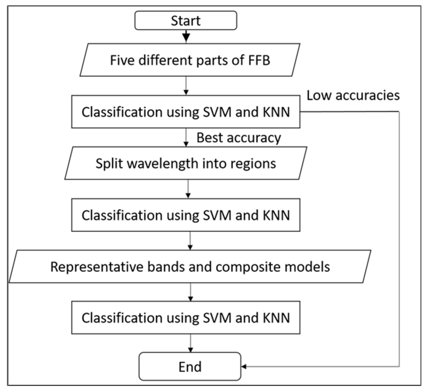
2.4. Support Vector Machine and K-Nearest Neighbor

Support vector machine is a classification algorithm that finds a 1-layer or multi-layer hyperplane for separable patterns. The data points nearest to the hyperplane are called support vectors. The support vectors have a direct impact on the hyperplane’s optimal position. The gap between two lines or hyperplanes is called a margin. Larger margin represents better classification. SVM’s main objective is to partition data sets into classes in order to find the greatest margin.

SVM offers a variety of benefits, including being successful when there are more features than training cases, being well-suited for extreme case classifications, and being the best method to employ when classes are separable. Only the support vectors affect the hyperplane; thus, outliers have less of an impact.

The K-nearest neighbor (KNN) model is frequently used in basic recommendation systems, image recognition, and decision-making models. Converting data points into feature vectors, or their mathematical values, is the first step in implementing KNN. The algorithm then determines the mathematical distance between these two points. The most popular technique for determining this distance is the Euclidean distance, as demonstrated below:

$$d (p, q)=d (q, p)=\sqrt{{\left(q_1-p_1\right)}^2+{\left(q_2-p_2\right)}^2+\cdots +{\left(q_n-p_n\right)}^2}$$

$$=\sqrt{{{\displaystyle \sum }}_{i=1}^n{\left(q_1-p_1\right)}^2}$$

where p and q are points on the plane. The Euclidean distance applied the theory of Pythagoras’ theorem to calculate distance values.

The classification training and testing were done in MATLAB R2020a. In MATLAB, the K-fold cross-validation function was applied, and 5-fold was chosen. This method divides the data into five separate parts. Each part was used as testing set and the other part acted as the training set. Then, the process was repeated until all five parts were used as testing set. The average of the accuracy is the overall accuracy for the classification.

3. Results

3.1. Principal Component Analysis and ANOVA

Table 5. Number of extracted PCs and variance percentage.

Parts	No. of PC Extracted	Percentage of Variance Explained
Front equatorial	1	92.4%
Front basil	5	90.6%
Back equatorial	5	90.3%
Back basil	5	89.8%
Apical	5	90.2%

shows the number of PCs extracted and the total percentage of variance explained by the PC for every part of FFB. For front equatorial, one PC was extracted with a 92.4% variance. For front basil, five PCs were extracted, with 90.6% variance explained. For back equatorial, five PCs were also extracted, with 90.3% variance. For back basil, five PCs were again extracted, with a variance of 89.8%. For apical, five PCs with a total of 90.2% variance were extracted.

The ANOVA test result for the front equatorial, using extracted PC, was shown in

Table 6. ANOVA test for front equatorial.

Robust Tests of Equality of Means
	Statistica	df1	df2	Sig.
Welch	38.585	2	52.792	0.000

; the significance level, or p-value, was less than 0.05. The null hypothesis was rejected, and there were statistically significant differences between the means of the three classes.

Table 7. ANOVA test for front basil.

		Sum of Squares	df	Mean Square	F	Sig.
PC 1	Between Groups	2.580	2	1.290	1.298	0.278
	Within Groups	92.420	93	0.994
PC 2	Between Groups	0.008	2	0.004	0.004	0.996
	Within Groups	94.992	93	1.021
PC 3	Between Groups	38.270	2	19.135	31.368	0.000
	Within Groups	56.730	93	0.610
PC 4	Between Groups	6.300	2	3.150	3.303	0.041
	Within Groups	88.700	93	0.954
PC 5	Between Groups	3.175	2	1.588	1.608	0.206
	Within Groups	91.825	93	0.987

shows the results of the ANOVA test for front basil. We can see that PC 1, PC 2, and PC 5 have a p value greater than 0.05. PC 3 and PC 4 have a p value of less than 0.05. PC 1 has the greatest variance explained, at 63.5%. Its p value is 0.278. Thus, we can say that there is no statistically significant difference between the three maturity groups based on the front basil.

Table 8. ANOVA test for back equatorial.

		Sum of Squares	df	Mean Square	F	Sig.
PC 1	Between Groups	8.481	2	4.240	4.672	0.012
	Within Groups	84.408	93	0.908
PC 2	Between Groups	1.750	2	0.875	0.872	0.421
	Within Groups	93.256	93	1.003
PC 3	Between Groups	33.160	2	16.580	24.694	0.000
	Within Groups	62.444	93	0.671
PC 4	Between Groups	1.768	2	0.884	0.886	0.416
	Within Groups	92.803	93	0.998
PC 5	Between Groups	2.390	2	1.195	1.188	0.309
	Within Groups	93.503	93	1.005

shows the results of the ANOVA test for back equatorial. PC 2, PC 4, and PC 5 have p values greater than 0.05. PC 1 and PC 3 have p values of less than 0.05. PC 1 has the greatest variance explained, which is 68.6%. Its p value is 0.012. Thus, we can say that there is a statistically significant difference between the three maturity groups based on the back equatorial.

Table 9. ANOVA test for back basil.

ANOVA
		Sum of Squares	df	Mean Square	F	Sig.
PC 1	Between Groups	10.080	2	5.040	5.519	0.005
	Within Groups	84.920	93	0.913
PC 2	Between Groups	7.199	2	3.600	3.813	0.026
	Within Groups	87.801	93	0.944
PC 3	Between Groups	8.784	2	4.392	4.737	0.011
	Within Groups	86.216	93	0.927
PC 4	Between Groups	7.386	2	3.693	3.920	0.023
	Within Groups	87.614	93	0.942
PC 5	Between Groups	2.704	2	1.352	1.362	0.261
	Within Groups	92.296	93	0.992

shows the results of the ANOVA test for back basil. We can see that PC 1, PC 2, PC 3, and PC 4 have p values of less than 0.05. PC 4 has a p value of less than 0.05. Thus, we can say that there is a statistically significant difference between the three maturity classes based on the back basil.

Table 10. ANOVA test for apical.

ANOVA
		Sum of Squares	df	Mean Square	F	Sig.
PC 1	Between Groups	14.165	2	7.082	8.148	0.001
	Within Groups	80.835	93	0.869
PC 2	Between Groups	4.243	2	2.121	2.174	0.119
	Within Groups	90.757	93	0.976
PC 3	Between Groups	22.064	2	11.032	14.067	0.000
	Within Groups	72.936	93	0.784
PC 4	Between Groups	1.933	2	0.966	0.966	0.385
	Within Groups	93.067	93	1.001
PC 5	Between Groups	0.554	2	0.277	0.273	0.762
	Within Groups	94.446	93	1.016

shows the results of the ANOVA test for apical. We can see that PC 1 and PC 3 have p values of less than 0.05. PC 2, PC 4, and PC 5 have p values of less than 0.05. PC 1 explains 66% of the variance. Thus, we can say that there is a statistically significant difference between the three maturity categories based on the apical.

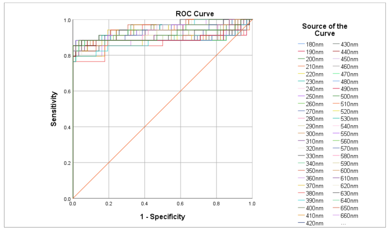
3.2. Classification Using All Bands from 180 to 1100 nm

The classification accuracies of each part are shown in

Table 11. Classification accuracy using all bands from 180 to 1100 nm.

	Classification Accuracy (%)
	Classifiers
Parts	KNN	SVM
Apical	68.4	74.5
Front equatorial	87.5 *	90.6 *
Front basil	69.1	71.3
Back equatorial	60.2	69.4
Back basil	65.6	66.4

Note: The asterisks mark the highest accuracies of each column.

. In the first mode, by using all bands as input to the classifiers, the results show that the front equatorial successfully achieved an average accuracy of above 89%. The accuracies of front equatorial were the highest in both classifiers. This is the best performance among the five parts. SVM produced the highest accuracy, which is 90.6%, followed by 87.5% produced by KNN. Back basil achieved the lowest classification accuracy in SVM, at 66.4%. Back equatorial achieved the lowest classification accuracy, at 60.2%, in KNN.

The receiver operating characteristic (ROC) curve is illustrated below in Figure 5. It describes the accuracy performance of the classification of front equatorial. It is a graph of sensitivity against specificity. Curves that are closer to the top-left corner represent better performances. The diagonal line is drawn across the middle of the graph. The closer the curves to the diagonal line, the less accurate it is. To compare different curve performances, the area under the curve (AUC) can be utilized. AUC, a measure of a model’s ability to discriminate between classes, is frequently used to summarize ROC curves [43]. The higher the value of AUC, the better the performance of the model.

The mean AUC is 0.908, with a 95% confidence interval. The highest AUC value is contributed by the 350 nm curve with a value of 0.959, whereas the lowest AUC value comes from the 680 nm curve with a value of 0.865. The mean lower bound is 0.824, while the upper bound is 0.992. This shows a promising result for the classification of the front equatorial data.

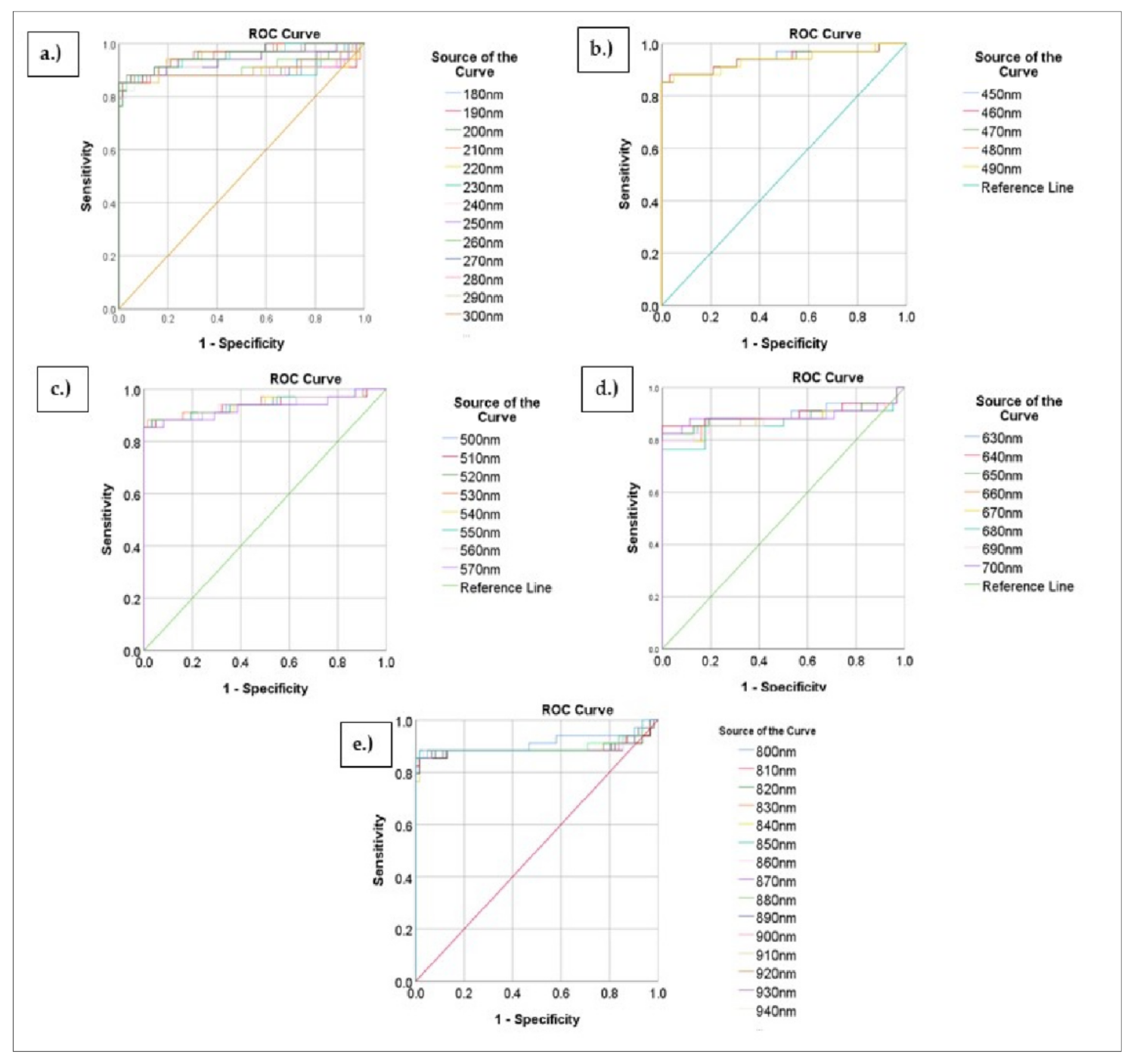
3.3. Classification Using Different Bands

In the second mode of classification, wavelengths were divided into UV, visible, and NIR bands for individual classification testing. The front equatorial data set was used in this mode as it shows a better result compared to others. The results are shown in

Table 12. Classification accuracies for different wavelength bands.

	Classification Accuracy (%)
	Classifiers
Regions	KNN	SVM
UV	87.5 *	91.7 *
Blue	87.5 *	87.5
Green	82.3	69.8
Red	78.1	76.0
NIR	84.4	78.1

Note: The asterisks mark the highest accuracies of each column.

. By using KNN as classifiers, UV and Blue achieved the highest accuracy level of 87.5%. Meanwhile, red bands have the lowest accuracy of 78.1%. By using SVM as classifiers, UV bands have the highest accuracy level of 91.7%, and green bands have the lowest accuracy level of 69.8%.

The ROC curve was drawn to test the accuracy performance of each region. Figure 6a shows the ROC curve of the UV bands. The mean AUC is 0.922 with a 95% confidence interval. The highest AUC value is contributed by the 350 nm curve with a value of 0.959, and the lowest AUC value comes from the 210 nm curve with a value of 0.889. The mean lower bound is 0.849, while the upper bound is 0.995.

Figure 6b shows the ROC curve of the blue bands. The mean AUC is 0.941, with a 95% confidence interval. The highest AUC value is contributed by the 450 nm curve with a value of 0.944, and the lowest AUC value comes from the 490 nm curve with a value of 0.938. The mean lower bound is 0.879, while the upper bound is 1.000.

Figure 6c shows the ROC curve of the green bands. The mean AUC is 0.939, with a 95% confidence interval. The highest AUC value is contributed by the 530 nm curve with a value of 0.944, and the lowest AUC value comes from the 570 nm curve with a value of 0.930. The mean lower bound is 0.875, while the upper bound is 0.999.

Figure 6d shows the ROC curve of the red bands. The mean AUC is 0.884, with a 95% confidence interval. The highest AUC value is contributed by the 640 nm curve with a value of 0.899, and the lowest AUC value comes from the 680 nm curve with a value of 0.865. The mean lower bound is 0.789, while the upper bound is 0.979.

Figure 6e shows the ROC curve of the NIR bands. The mean AUC is 0.891, with a 95% confidence interval. The highest AUC value is contributed by the 1100 nm curve with a value of 0.914, and the lowest AUC value comes from the 990–1020 nm curve with a value of 0.885. The mean lower bound is 0.792, while the upper bound is 0.989.

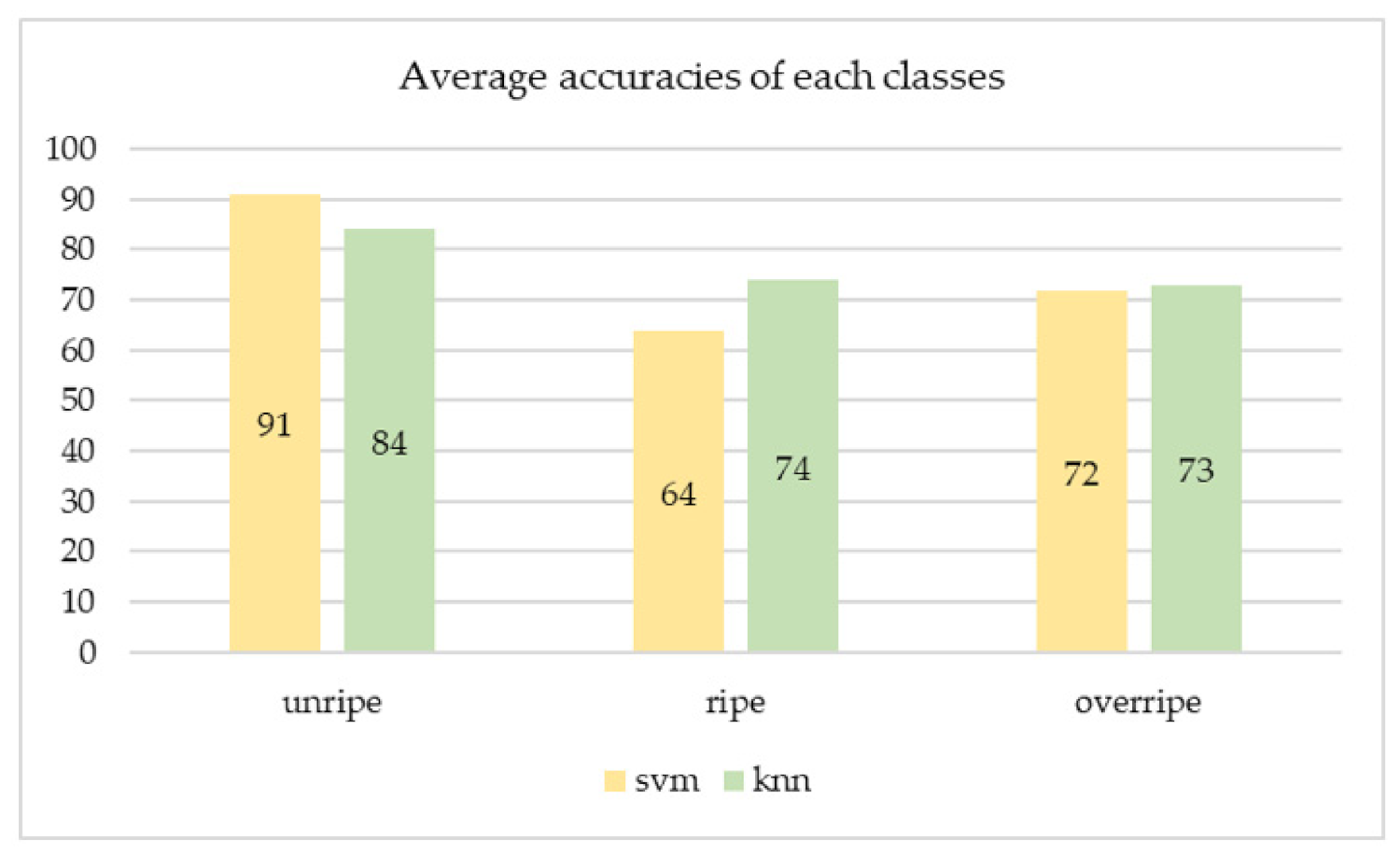
3.4. Classification Using Representative Bands

The classification accuracies of the third mode, which used representative bands, are shown in

Table 13. Classification accuracy using representative bands.

	Classification Accuracy (%)
	Classifiers
Bands (nm)	KNN	SVM
365	87.5	79.2
460	84.4	74.0
523	75.0	65.6
590	80.2	68.8
623	82.3	60.4
660	89.6 *	69.8
735	88.5	71.9
850	78.1	72.9

Note: The asterisks mark the highest accuracies of each column.

. These bands were extracted from the UV, blue, green, amber, red, deep red, far-red, and near-infrared regions, respectively, via front equatorial, as it has the best accuracy. By using KNN as the classifier, 660 nm (deep red) has the highest accuracy, at 89.6%, whereas 523 nm has the lowest accuracy, at 75.0%. By using all the representative bands in the KNN analysis, the composite model shows an accuracy of 92.7%. If the 523 nm band is removed from the combination, the accuracy drops slightly to 91.7%. The accuracy is maintained at 92.7% by removing the 850 nm (near-infrared) band from the combination. Meanwhile, in the SVM classification, 365 nm (UV) has the highest accuracy, at 79.2%, whereas 623 nm (red) has the lowest accuracy, at 60.4%. By using combinations of all the representative bands in the SVM analysis, the accuracy reaches 92.7%. The classification accuracy is increased to 93.8% if bands 523, 590, 623, and 660 nm are removed from the combination. Note that these four bands each have an accuracy lower than 70%. The composite models and their accuracies are shown in

Table 14. Classification accuracy using composite models.

Classifiers	Combination of Bands (nm)	Accuracies (%)
KNN	365, 460, 523, 590, 623, 660, 735, 850	92.7 *
	365, 460, 590, 623, 660, 735, 850	91.7
	365, 460, 523, 590, 623, 660, 735	92.7 *
	365, 460, 590, 623, 660, 735,	91.7
SVM	365, 460, 523, 590, 623, 660, 735, 850	92.7
	365, 523, 590, 623, 660, 735, 850	92.7
	365, 460, 523, 623, 660, 735, 850	92.7
	365, 460, 735, 850	93.8 *

Note: The asterisks mark the highest accuracies of each column.

.

The average accuracy of KNN is 79.2%, whereas the average accuracy of SVM is 75.5%. This shows that KNN has a better performance than SVM. Meanwhile, Figure 7 shows the comparison between the average accuracies of three maturity levels. The unripe class has better average accuracies compared to the other classes.

4. Discussion

ANOVA tests showed that, except for the front basil, the other four parts of the FFB, i.e., the front equatorial, back equatorial, back basil, and apical, exhibited statistical differences between the three maturity groups. The front equatorial was identified as the best part to determine the FFB maturity level. It had the highest classification accuracies of 87.5% and 90.6%, using KNN and SVM, respectively. This could be due to the growing condition of the FFB on the oil palm tree where the front equatorial faced the direction of sunlight and photosynthesis occurred regularly. Compared to the backside of the FFB, where it faced the tree and did not receive enough sunlight for photosynthesis, back basil and back equatorial both had the lowest accuracies in KNN and SVM classifications. The back basil part was constantly concealed by the fronds of the tree and was often yellowish or greenish in color. Junkwon et al. [44] mentioned that the color of back basil fruits significantly varies by variety and planting location. Hence, it was impractical for use.

The classification of FFB using reflectance intensity is a popular method in this field. Junkwon et al. [21] concluded that hyperspectral data has better potential than RGB images to classify the FFB maturity level. It is an NDM method focusing on special characteristics of the reflectance data to discover the relationship between them and the maturity level of FFB. For example, Junkwon et al. [44] described the application of the hyperspectral camera in discovering the internal qualities of FFB. They found that the 960 to 990 nm wavelength was suitable for maturity classification. Bensaeed et al. [27] used a hyperspectral-base system and found that 750–910 nm bands can distinguish the three classes of maturity clearly. These bands were in the NIR region. Their results share a similarity with our results, where the NIR region achieved 84.4% accuracy using KNN as a classifier.

Saeed et al. [22] stated that 570, 670, 750, and 870 nm were robust in classifying FFB maturity with 85% accuracy. These four bands fall within the green to NIR regions. In this study, the green region has 82.3% accuracy, the red region has 78.1% accuracy, and the NIR region has 84.4% accuracy in the FFB maturity classifications. This is consistent with previous research findings. In fact, the four bands were extracted in this research’s data set for classification to compare with Saeed et al. [22] results. Using SVM as a classifier resulted in greater accuracy, at 90.6%.

In the classification of each region, the UV region from 180 nm to 400 nm had the highest maturity classification accuracy, of 87.5% using KNN and 91.7% using SVM. The AUC of this was 0.922, thus further proving the performance of the UV band. The Kappa coefficient also supported this performance with a value of 0.86. This finding agreed with the results of Cherie et al. [45], where the UV lamp with 320–380 nm could determine the most suitable harvest decision for FFB on the tree.

Composite models using extracted bands show better performance compared to Dayaf [15], in which the best composite model was 590 and 660 nm, with 85.7% accuracy. In this current research, the combination of 365, 460, 735, and 850 nm wavelengths achieved an accuracy of 93.8% by using SVM, which is higher than the Dayaf [15] model’s accuracy. Furthermore, this composite model also surpassed the accuracy of all band classifications with 90.6% for the front equatorial data set and 91.7% for the UV region. This was the highest accuracy in the three modes of classification in this study.

This research uses three modes to classify FFB maturity. We tried to reduce the number of bands for classification without losing accuracy and found that the UV region containing 23 bands, from 180 to 400 nm, improved the accuracy by 1% only. On the other hand, the composite model of 365, 460, 735, and 850 nm improved the accuracy to 93.8%, despite using only four bands.

Two types of classifiers, SVM and KNN, were used in the analysis. In the first mode of analysis, SVM surpassed the performances of KNN, with the former producing 90.6% of accuracy for the front equatorial and the latter only producing an accuracy of 87.5%. In fact, SVM produced greater accuracy for apical, front equatorial, front basil, back equatorial, and back basil than KNN. In the second mode of analysis, SVM produced the highest accuracy for the UV regions, at 91.7%, while KNN produced an accuracy of 87.5%. In the third mode of analysis, where representative bands were used as inputs, KNN outperformed SVM with the highest accuracy of 89.6% for 660 nm, whereas SVM produced an accuracy of 69.8%. Nevertheless, SVM still produced the best overall performance for the composite model of (365, 460, 735, and 850 nm) with 93.8% accuracy. In short, both SVM and KNN are robust in the classification analysis. SVM is computationally less intensive than KNN and easier to understand, but it recognizes a limited number of patterns. KNN, on the other hand, can find extremely complicated patterns, but its output is more difficult to understand [46]. Sabri et al. [47] proved the efficiency of SVM in FFB grading using color features where SVM produced accuracies from between 70% to 96%. Alfatni et al. [48] also proved that the classification accuracy of the statistical color feature extraction from FFB with the SVM classifier was at 92%, and the color histogram feature extraction with the SVM classifier was at 92% as well. Our performance of KNN was also slightly higher than the performance of KNN in the Dayaf [15] research, where it achieved 88.7% accuracy.

5. Conclusions

This study investigated oil palm FFB reflectance data. We proved that the optical spectrometer had the ability to determine oil palm FFB maturity levels. The utilization of all bands, from 180 to 1100 nm, resulted in 90.6% accuracy by using SVM as a classifier for the front equatorial. The front equatorial was identified as the prime part of FFB to focus on for the maturity data acquisition of the oil palm FFB. This vital discovery will be of immense aid to future researchers in expediting field data collection. The next important contribution of this research was the findings that the UV region alone produced an accuracy of 91.7% by using SVM. Finally, a composite model consisting of 365, 460, 735, and 850 nm produced the highest accuracy, at 93.8%. It can be concluded that, instead of all bands, we can reduce the number of bands to a specific region or specific bands for the classification of FFB maturity levels.

For future work, a simple sensor that consists of the above-selected regions or a composite model can be built to detect the maturity level of FFB to replace the existing human grading method.

References

1. Ebarcelos, E.; Rios, S.E.A.; Cunha, R.N.V.; Elopes, R.; Motoike, S.Y.; Ebabiychuk, E.; Eskirycz, A.; Kushnir, S. Oil palm natural diversity and the potential for yield improvement. Front. Plant Sci. 2015, 6, 190. [Google Scholar]
2. WWF. 8 Things to Know about Palm Oil. WWF. 2020. Available online: https://www.wwf.org.uk/updates/8-things-know-about-palm-oil (accessed on 3 March 2021).
3. EPOA. The Palm Oil Story; European Palm Oil Alliance: Zoetermeer, The Netherlands, 2019; pp. 1–16. [Google Scholar]
4. Tullis, P. How the World Got Hooked on Palm Oil. 2019. Available online: https://www.theguardian.com/news/2019/feb/19/palm-oil-ingredient-biscuits-shampoo-environmental (accessed on 3 March 2021).
5. Voora, V.; Larrea, C.; Bermudez, S.; Baliño, S. Global Market Report: Palm Oil. 2019. Available online: https://www.iisd.org/system/files/publications/ssi-global-market-report-palm-oil.pdf (accessed on 6 November 2021).
6. RSPO. Partnerships for innovation. In Proceedings of the RSPO 5th European Roundtable 2017, London, UK, 13 June 2017. [Google Scholar]
7. EPOA. Latest Data Shows 86% of Palm Oil Imported to Europe Sustainable; Sustainable Palm Oil for Europe in 2019; EPOA: Zoetermeer, The Netherlands, 2019; Available online: https://www.idhsustainabletrade.com/news/latest-data-shows-86-of-palm-oil-imported-to-europe-sustainable/ (accessed on 6 April 2021).
8. Makky, M.; Soni, P.; Salokhe, V.M. Automatic non-destructive quality inspection system for oil palm fruits. Int. Agrophys. 2014, 28, 319–329. [Google Scholar] [CrossRef] [Green Version]
9. Peng, T.S.; Shafie, H.Z. Panduan Penggredan Buah Tandan Segar Sawit Untuk Pekebun Kecil. Kajang, Selangor. 2015. Available online: http://palmoilis.mpob.gov.my/V4/wp-content/uploads/2021/05/Risalah-31.pdf (accessed on 1 August 2021).
10. Chauhan, O.P.; Lakshmi, S.; Pandey, A.K.; Ravi, N.; Gopalan, N.; Sharma, R.K. Non-destructive Quality Monitoring of Fresh Fruits and Vegetables. Def. Life Sci. J. 2017, 2, 103–110. [Google Scholar] [CrossRef]
11. Zulkifli, A.B.H.Z.M.; Hashim, F.H.; Raj, T. A Rapid and Non-Destructive Technique in Determining the Ripeness of Oil Palm Fresh Fruit Bunch (FFB). J. Kejuruter. 2018, 30, 93–101. [Google Scholar]
12. Utom, S.L.; Mohamad, E.J.; Ameran, H.L.M.; Kadir, H.A.; Muji, S.Z.M.; Rahim, R.A.; Pusppanathan, J. Non-Destructive Oil Palm Fresh Fruit Bunch (FFB) Grading Technique Using Optical Sensor. Int. J. Integr. Eng. 2018, 10, 35–39. [Google Scholar]
13. Makky, M. A Portable Low-cost Non-destructive Ripeness Inspection for Oil Palm FFB. Agric. Agric. Sci. Procedia 2016, 9, 230–240. [Google Scholar] [CrossRef] [Green Version]
14. Shiddiq, M.; Fitmawati; Anjasmara, R.; Sari, N. Hefniati Ripeness detection simulation of oil palm fruit bunches using laser-based imaging system. AIP Conf. Proc. 2017, 1801, 050003. [Google Scholar]
15. Dayaf, A.A.H.B. Oil Palm Fresh Fruit Bunches Maturity Classification and Oil Analysis Correlation. Ph.D. Thesis, UPM, Seri Kembangan, Malaysia, 2017. [Google Scholar]
16. Setiawan, A.W.; Mengko, R.; Putri, A.P.H.; Danudirdjo, D.; Ananda, A.R. Classification of palm oil fresh fruit bunch using multiband optical sensors. Int. J. Electr. Comput. Eng. 2019, 9, 2386–2393. [Google Scholar] [CrossRef]
17. Zolfagharnassab, S.; Shariff, A.R.M.; Ehsani, R. Emissivity determination of oil palm fresh fruit ripeness using a thermal imaging technique. Acta Hortic. 2017, 1152, 189–193. [Google Scholar] [CrossRef]
18. Misron, N.; Azhar, N.S.K.; Hamidon, M.N.; Aris, I.; Tashiro, K.; Nagata, H. Fruit battery with charging concept for oil palm maturity sensor. Sensors 2020, 20, 226. [Google Scholar] [CrossRef] [PubMed] [Green Version]
19. Shabdin, M.K.; Shariff, A.R.M.; Johari, M.N.A.; Saat, N.K.; Abbas, Z. A study on the oil palm fresh fruit bunch (FFB) ripeness detection by using Hue, Saturation and Intensity (HSI) approach. IOP Conf. Ser. Earth Environ. Sci. 2016, 37, 012039. [Google Scholar] [CrossRef]
20. Hazir, M.H.M.; Shariff, A.R.M.; Amiruddin, M.D. Determination of oil palm fresh fruit bunch ripeness—Based on flavonoids and.pdf. Ind. Crop. Prod. 2012, 36, 466–475. [Google Scholar] [CrossRef]
21. Junkwon, P.; Takigawa, T.; Okamoto, H.; Hasegawa, H.; Koike, M.; Sakai, K.; Siruntawineti, J.; Chaeychomsri, W.; Sanevas, N.; Tittinuchanon, P.; et al. Potential Application of Color and Hyperspectral Images for Estimation of Weight and Ripeness of Oil Palm (Elaeis guineensis Jacq. var. tenera). Agric. Inf. Res. 2009, 18, 72–81. [Google Scholar] [CrossRef]
22. Saeed, O.; Sankaran, S.; Shariff, A.R.M.; Shafri, H.Z.M.; Ehsani, R.; Alfatni, M.S.; Hazir, M.H.M. Classification of oil palm fresh fruit bunches based on their maturity using portable four-band sensor system. Comput. Electron. Agric. 2012, 82, 55–60. [Google Scholar] [CrossRef]
23. Hafiz, M.; Shariff, A.R.M. Oil palm physical and optical characteristics from two different: Planting materials. Res. J. Appl. Sci. Eng. Technol. 2011, 3, 953–962. [Google Scholar]
24. Jamil, N.; Mohamed, A.; Abdullah, S. Automated grading of palm oil Fresh Fruit Bunches (FFB) using neuro-fuzzy technique. In Proceedings of the 2009 International Conference of Soft Computing and Pattern Recognition, Malacca, Malaysia, 4–7 December 2009; pp. 245–249. [Google Scholar]
25. May, Z.; Amaran, M.H. Automated Oil Palm Fruit Grading System using Artificial Intelligence. Int. J. Eng. Sci. 2011, 11, 30–35. [Google Scholar]
26. Fadilah, N.; Mohamad-Saleh, J.; Halim, Z.A.; Ibrahim, H.; Ali, S.S.S. Intelligent color vision system for ripeness classification of oil palm fresh fruit bunch. Sensors 2012, 12, 14179–14195. [Google Scholar] [CrossRef]
27. Bensaeed, O.M.; Shariff, A.M.; Mahmud, A.B.; Shafri, H.; Alfatni, M. Oil palm fruit grading using a hyperspectral device and machine learning algorithm. IOP Conf. Ser. Earth Environ. Sci. 2014, 20, 012017. [Google Scholar] [CrossRef]
28. Ali, M.M.; Hashim, N.; Hamid, A.S.A. Combination of laser-light backscattering imaging and computer vision for rapid determination of oil palm fresh fruit bunches maturity. Comput. Electron. Agric. 2020, 169, 105235. [Google Scholar]
29. Ivanciuc, O. Applications of support vector machines in chemistry. Rev. Comput. Chem. 2007, 23, 291–400. [Google Scholar]
30. Harrison, O. Machine Learning Basics with the K-Nearest Neighbors Algorithm. Towards Data Science. 2018. Available online: https://towardsdatascience.com/machine-learning-basics-with-the-k-nearest-neighbors-algorithm-6a6e71d01761 (accessed on 1 August 2021).
31. Liakos, K.G.; Busato, P.; Moshou, D.; Pearson, S.; Bochtis, D. Machine learning in agriculture: A review. Sensors 2018, 18, 2674. [Google Scholar] [CrossRef] [PubMed] [Green Version]
32. Khan, N.; Kamaruddin, M.A.; Sheikh, U.U.; Yusup, Y.; Bakht, M.P. Oil palm and machine learning: Reviewing one decade of ideas, innovations, applications, and gaps. Agriculture 2021, 11, 832. [Google Scholar] [CrossRef]
33. Sengupta, S.; Lee, W.S. Identification and determination of the number of immature green citrus fruit in a canopy under different ambient light conditions. Biosyst. Eng. 2014, 117, 51–61. [Google Scholar] [CrossRef]
34. Ramos, P.J.; Prieto, F.A.; Montoya, E.C.; Oliveros, C.E. Automatic fruit count on coffee branches using computer vision. Comput. Electron. Agric. 2017, 137, 9–22. [Google Scholar] [CrossRef]
35. Chung, C.L.; Huang, K.J.; Chen, S.Y.; Lai, M.H.; Chen, Y.C.; Kuo, Y.F. Detecting Bakanae disease in rice seedlings by machine vision. Comput. Electron. Agric. 2016, 121, 404–411. [Google Scholar] [CrossRef]
36. Nooni, I.K.; Duker, A.A.; van Duren, I.; Addae-Wireko, L.; Jnr, E.M.O. Support vector machine to map oil palm in a heterogeneous environment. Int. J. Remote Sens. 2014, 35, 4778–4794. [Google Scholar] [CrossRef]
37. Zolfagharnassab, S. Application of Thermal Imaging Technique to Quantify the Oil Palm Fresh Fruit Maturity, Oil Content and Oil Quality Parameters. Ph.D. Thesis, UPM, Seri Kembangan, Malaysia, 2019. [Google Scholar]
38. NASA. Electromagnetic Spectrum-Introduction; High Energy Astrophysics Science Archive Research Center. 2013. Available online: https://imagine.gsfc.nasa.gov/science/toolbox/emspectrum1.html#:~:text=The%20Electromagnetic%20Spectrum,two%20types%20of%20electromagnetic%20radiation (accessed on 15 May 2021).
39. Kassim, M.S.M.; Ismail, W.I.W.; Teik, L.H. Oil palm fruit classifications by using near infrared images. Res. J. Appl. Sci. Eng. Technol. 2014, 7, 2200–2207. [Google Scholar] [CrossRef]
40. Morais, R.; Mendes, J.; Silva, R.; Silva, N.; Sousa, J.J.; Peres, E. A versatile, low-power and low-cost IoT device for field data gathering in precision agriculture practices. Agriculture 2021, 11, 619. [Google Scholar] [CrossRef]
41. Kayad, A.; Paraforos, D.S.; Marinello, F.; Fountas, S. Latest advances in sensor applications in agriculture. Agriculture 2020, 10, 362. [Google Scholar] [CrossRef]
42. Shariff, A.R.B.M.; Nawi, N.M. Ripeness Classification of Oil Palm Fresh Fruit Bunches Using Optical Spectrometer and Support Vector Machine. In Proceedings of the 2021 ASABE Annual International Virtual Meeting, Online. 17–20 July 2021; American Society of Agricultural and Biological Engineers: St. Joseph, MI, USA, 2021; p. 1. Available online: https://elibrary.asabe.org/techpapers.asp?confid=virt2021 (accessed on 15 May 2021).
43. Bhandari, A. AUC-ROC Curve in Machine Learning Clearly Explained—Analytics Vidhya. 2020. Available online: https://www.analyticsvidhya.com/blog/2020/06/auc-roc-curve-machine-learning/ (accessed on 15 May 2021).
44. Junkwon, P.; Takigawa, T.; Okamoto, H.; Hasegawa, H.; Koike, M.; Sakai, K.; Siruntawineti, J.; Chaeychomsri, W.; Vanavichit, A.; Tittinuchanon, P.; et al. Hyperspectral imaging for nondestructive determination of internal qualities for oil palm (Elaeis guineensis Jacq. var. tenera). Agric. Inf. Res. 2009, 18, 130–141. [Google Scholar] [CrossRef] [Green Version]
45. Cherie, D.; Herodian, S.; Ahmad, U.; Mandang, T.; Makky, M. Optical characteristics of oil palm fresh fruits bunch (FFB) under three spectrum regions influence for harvest decision. Int. J. Adv. Sci. Eng. Inf. Technol. 2015, 5, 255–263. [Google Scholar]
46. Bzdok, D.; Krzywinski, M.; Altman, N. Machine learning: Supervised methods. Nat. Methods 2018, 15, 5–6. [Google Scholar] [CrossRef] [PubMed]
47. Sabri, N.; Ibrahim, Z.; Syahlan, S.; Jamil, N.; Mangshor, N.N.A. Palm oil fresh fruit bunch ripeness grading identification using color features. J. Fundam. Appl. Sci. 2017, 9, 563–579. [Google Scholar] [CrossRef] [Green Version]
48. Alfatni, M.S.M.; Shariff, A.R.M.; Abdullah, M.Z.; Marhaban, M.H.; Shafie, S.B.; Bamiruddin, M.D.; Saaed, O.M.B. Oil palm fresh fruit bunch ripeness classification based on rule-based expert system of ROI image processing technique results. In IOP Conference Series: Earth and Environmental Science; IOP Publishing: Bristol, UK, 2014; Volume 20, p. 012018. [Google Scholar]
Figure 1. SE Series Spectrometer.
Agriculture 11 01179 g001
Figure 2. Experimental setup.
Agriculture 11 01179 g002
Figure 3. Five different parts of FFB: (a) front equatorial; (b) front basil; (c) back equatorial; (d) back basil; (e) apical.
Agriculture 11 01179 g003
Figure 4. Flowchart of the analysis process.
Agriculture 11 01179 g004
Figure 5. ROC curve of front equatorial represents the performance of all bands.
Agriculture 11 01179 g005
Figure 6. ROC curve of: (a) UV bands; (b) blue bands; (c) green bands; (d) red bands; and (e) NIR bands.
Agriculture 11 01179 g006
Figure 7. Average accuracies of the three maturity levels.
Agriculture 11 01179 g007