Image Generation of Tomato Leaf Disease Identification Based on Adversarial-VAE

Abstract

The deep neural network-based method requires a lot of data for training. Aiming at the problem of a lack of training images in tomato leaf disease identification, an Adversarial-VAE network model for generating images of 10 tomato leaf diseases is proposed, which is used to expand the training set for training an identification model. First, an Adversarial-VAE model is designed to generate tomato leaf disease images. Then, a multi-scale residual learning module is used to replace single-size convolution kernels to enrich extracted features, and a dense connection strategy is integrated into the Adversarial-VAE networks to further enhance the image generation ability. The training set is expanded by the proposed model, which generates the same number of images by training 10,892 images of 10 leaves. The generated images are superior to those of InfoGAN, WAE, VAE, and VAE-GAN measured by the Frechet Inception Distance (FID). The experimental results show that using the extension dataset that is generated by the Adversarial-VAE model to train the Resnet identification model could improve the accuracy of identification effectively. The model proposed in this paper could generate enough images of tomato leaf diseases and provide a feasible solution for data expansion of tomato leaf disease images.

1. Introduction

Leaf disease identification is crucial to control the spread of diseases and advance healthy development of the tomato industry. Well-timed and accurate identification of diseases is the key to early treatment, and an important prerequisite for reducing crop loss and pesticide use. Unlike traditional machine learning classification methods that manually select features, deep neural networks provide an end-to-end pipeline to automatically extract robust features, which significantly improve the availability of leaf identification. In recent years, neural network technology has been widely applied in the field of plant leaf disease identification [1,2,3,4,5,6,7,8,9], which indicates that deep learning-based approaches have become popular. However, because the deep convolutional neural network (DCNN) has a lot of adjustable parameters, a large amount of labeled data is needed to train the model to improve its generalization ability of the model. Sufficient training images are an important requirement for models based on convolutional neural networks (CNNs) to improve generalization capability. There are little data about agriculture, especially in the field of leaf disease identification. Collecting large numbers of disease data is a waste of manpower and time, and labeling training data requires specialized domain knowledge, which makes the quantity and variety of labeled samples relatively small. Moreover, manual labeling is a very subjective task, and it is difficult to ensure the accuracy of the labeled data. Therefore, the lack of training samples is the main impediment for further improvement of leaf disease identification accuracy. How to train the deep learning model with a small amount of existing labeled data to improve the identification accuracy is a problem worth studying. In general, researchers usually solve this challenge by using traditional data augmentation methods [10]. In computer vision, it makes perfect sense to employ data augmentation, which can change the characteristics of a sample based on prior knowledge so that the newly generated sample also conforms to, or nearly conforms to, the true distribution of the data, while maintaining the sample label. Due to the particularity of image data, additional training data can be obtained from the original image through simple geometric transformation. Common data enhancement methods include rotation, scaling, translation, cropping, noise addition, and so on. However, little additional information can be obtained from these methods.

In recent years, data expansion methods based on generative models have become a research hotspot and have been applied in various fields [11,12,13,14,15]. For example, in [11], the author presents an approach for learning to translate an image from a source domain X to a target domain Y in the absence of paired examples to learn a mapping G: X→Y, such that the distribution of images from G(X) is indistinguishable from the distribution Y using an adversarial loss. Usually, the two most common techniques for training generative models are the generative adversarial network (GAN) [16] and variational auto-encoder (VAE) [17], both of which have advantages and disadvantages. Goodfellow et al. proposed the GAN model [16] for latent representation learning based on unsupervised learning. Through the adversarial learning of the generator and discriminator, fake data consistent with the distribution of real data can be obtained. It can overcome many difficulties, which appear in many tricky probability calculations of maximum likelihood estimation and related strategies. However, because the input z of the generator is a continuous noise signal and there are no constraints, GAN cannot use this z, which is not an interpretable representation. Radford et al. [18] proposed DCGAN, which adds a deep convolutional network based on GAN to generate samples, and uses deep neural networks to extract hidden features and generate data. The model learns the representation from the object to the scene in the generator and discriminator. InfoGAN [19] tried to use z to find an interpretable expression, where z is broken into incompressible noise z and interpretable implicit variable c. In order to make the correlation between x and c, it is necessary to maximize the mutual information. Based on this, the value function of the original GAN model is modified. By constraining the relationship between c and the generated data, c contains interpreted information about the data. In [20], Arjovsky et al. proposed Wasserstein GAN (WGAN), which uses the Wasserstein distance instead of Kullback-Leibler divergence to measure the probability distribution, to solve the problem of gradient disappearance, ensure the diversity of generated samples, and balance sensitive gradient loss between the generator and discriminator. Therefore, WGAN does not need to carefully design the network architecture, and the simplest multi-layer fully connected network can do it. 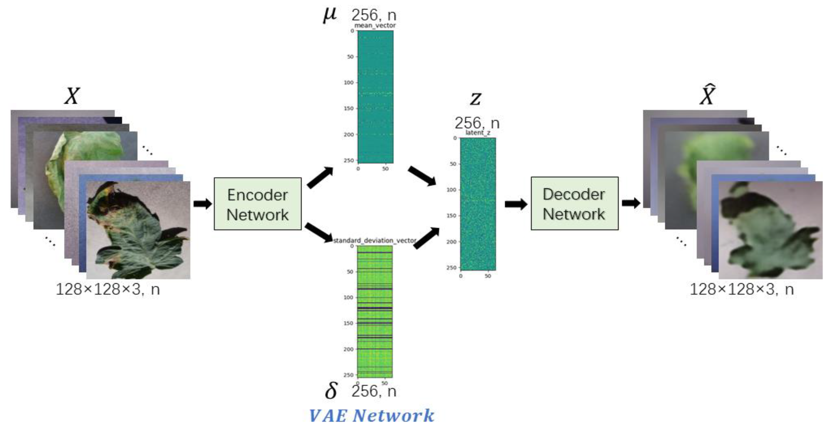In [17], Kingma et al. proposed a deep learning technique called VAE for learning latent expressions. VAE provides a meaningful lower bound for the log likelihood that is stable during training and during the process of encoding the data into the distribution of the hidden space. However, because the structure of VAE does not clearly learn the goal of generating real samples, it just hopes to generate data that is closest to the real samples, so the generated samples are more ambiguous. In [21], the researchers proposed a new generative model algorithm named WAE, which minimizes the penalty form of the Wasserstein distance between the model distribution and the target distribution, and derives the regularization matrix different from that of VAE. Experiments show that WAE has many characteristics of VAE, and it generates samples of better quality as measured by FID scores at the same time. Dai et al. 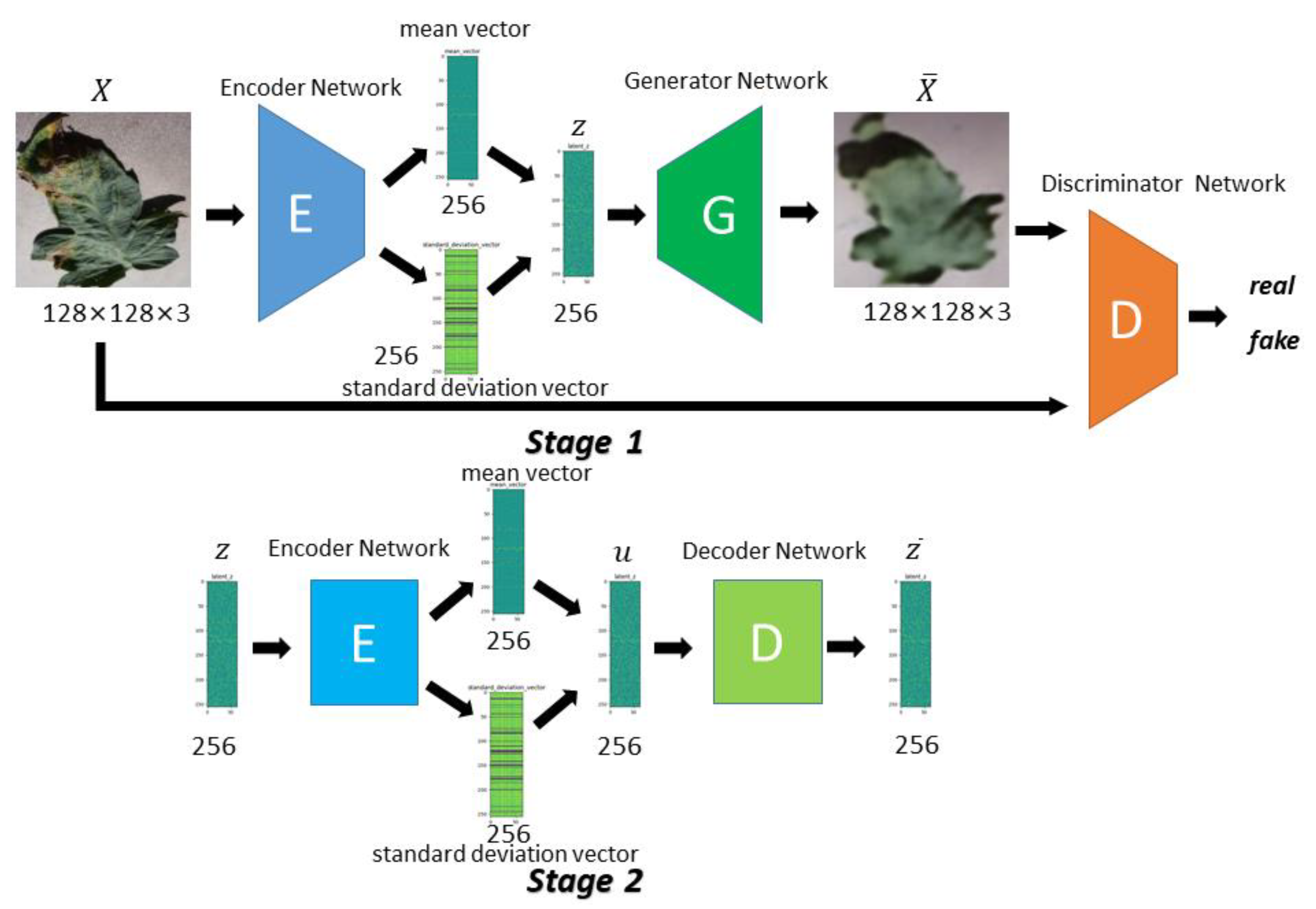[22] analyzed the reasons for the poor quality of VAE generation and concluded that although it could learn data manifold, the specific distribution in the manifold it learns is different from the real distribution. In the experiment, it shows that VAE can reconstruct training data well, but it cannot generate new samples well. Therefore, a two-stage VAE is proposed, where the first one is used to learn the position of the manifold, and the second is used to learn the specific distribution within the manifold, which improves the generation effect significantly.

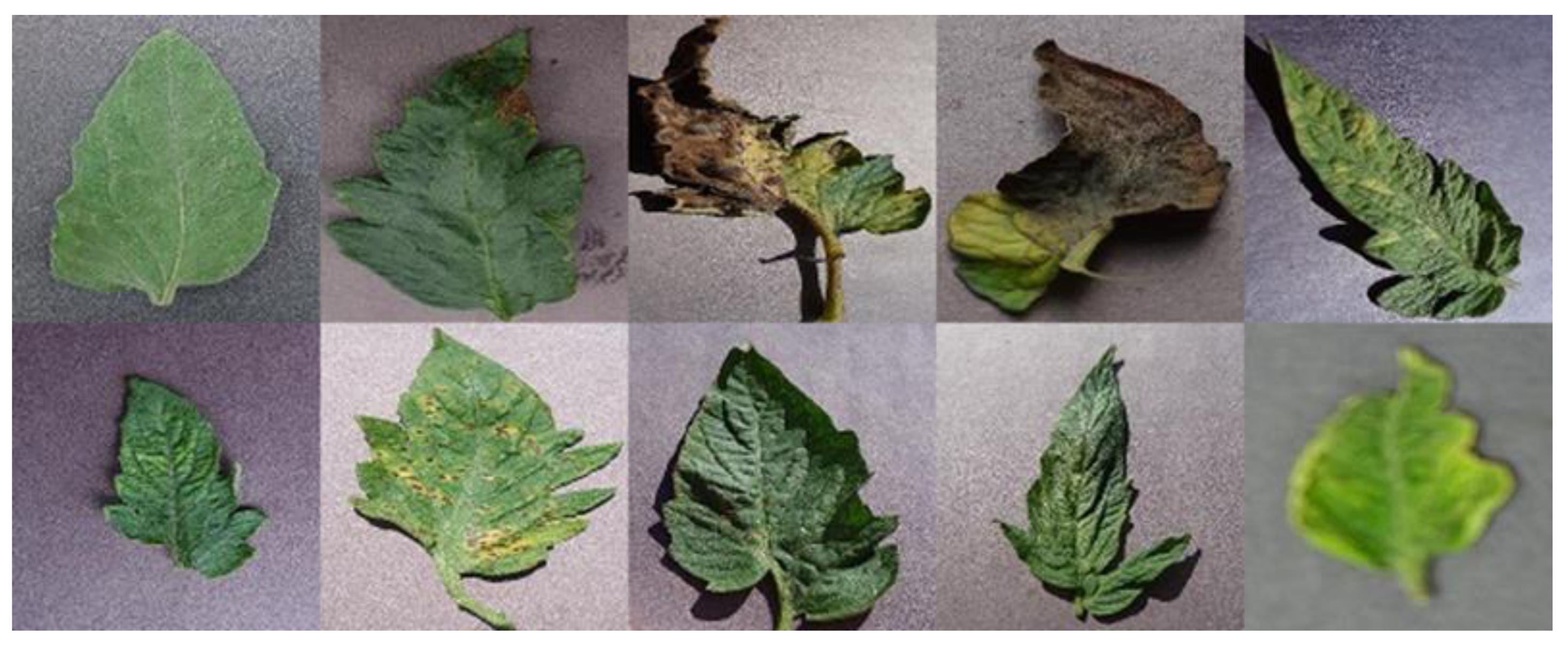
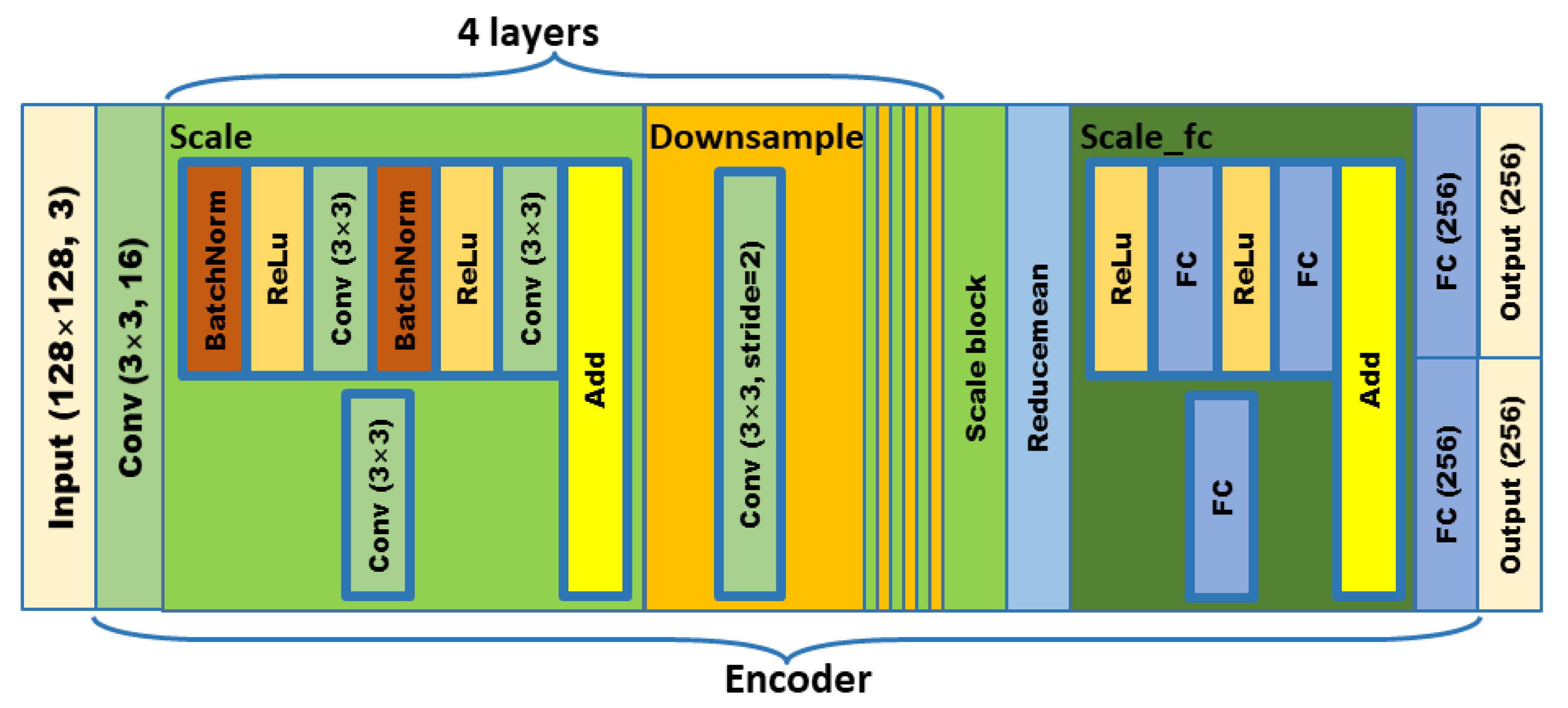
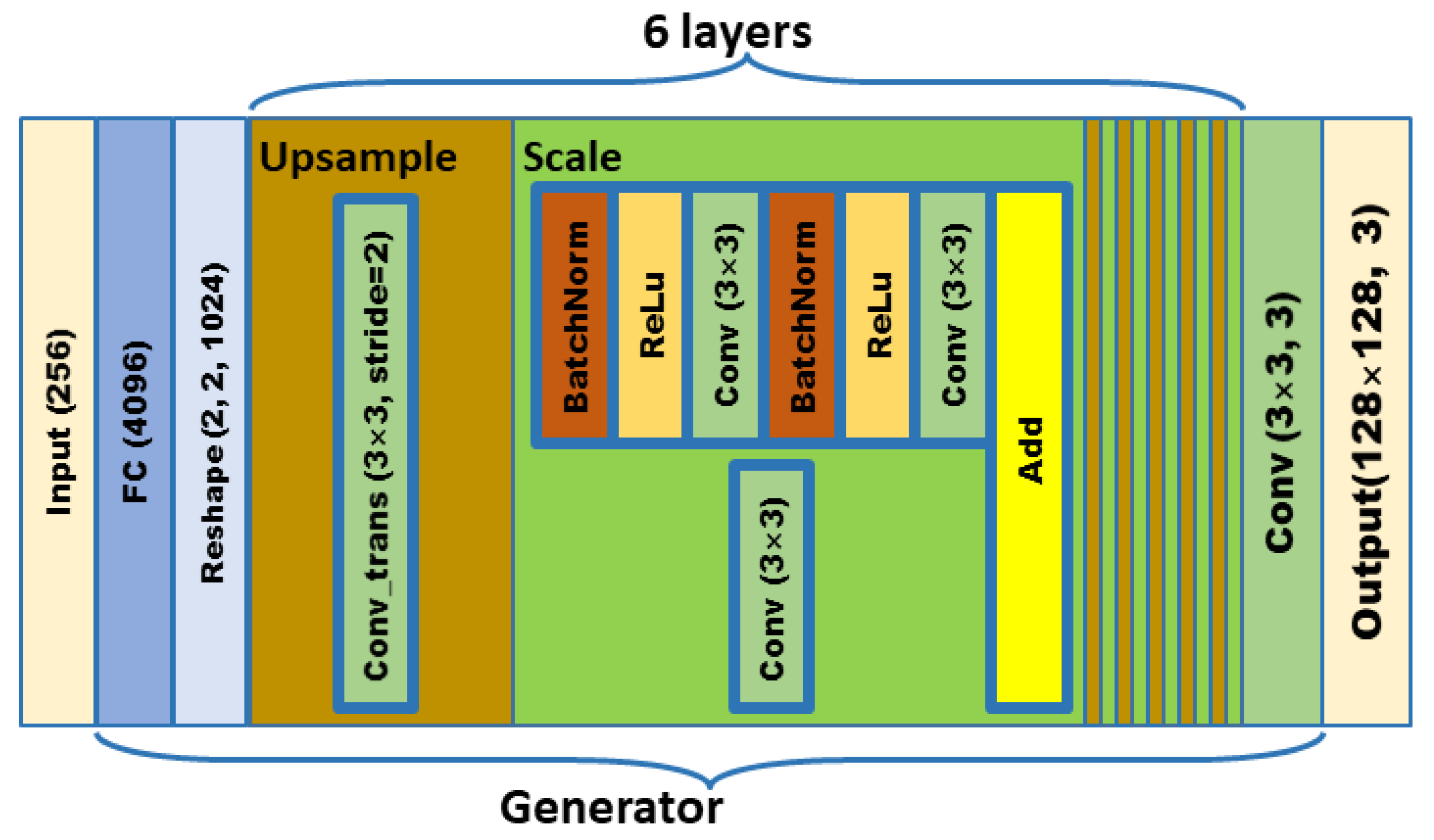
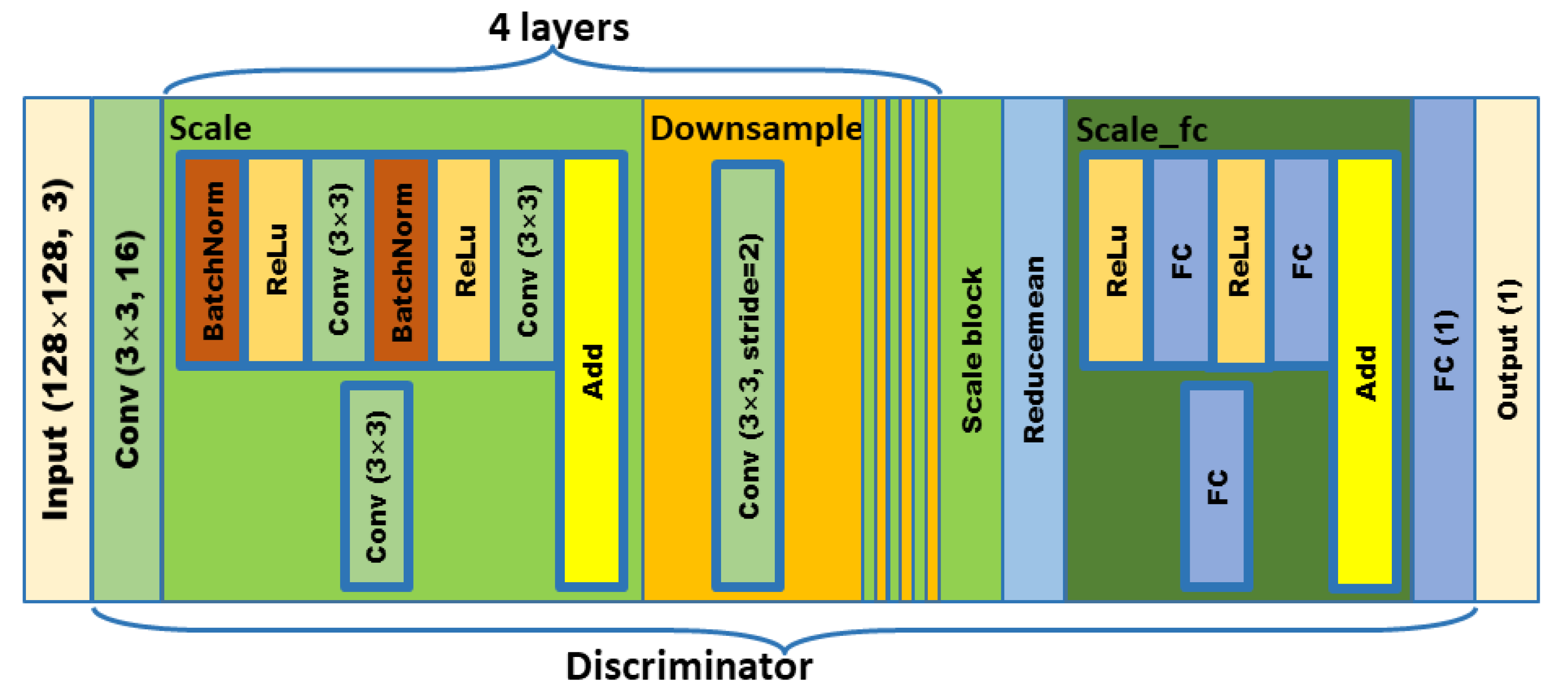
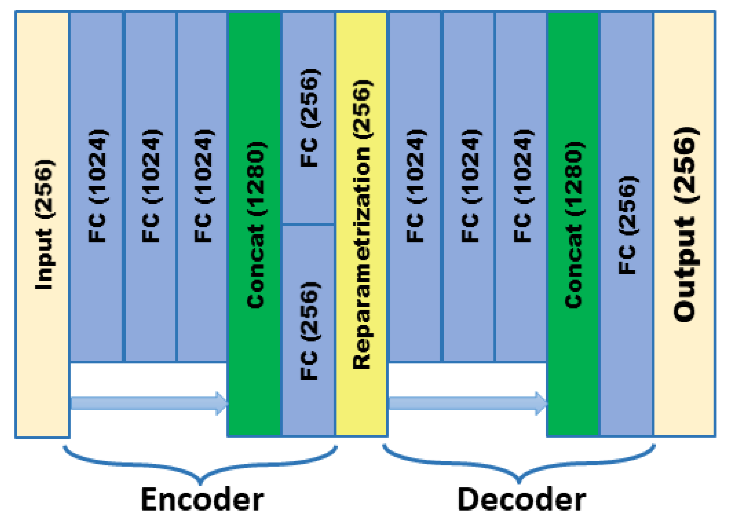
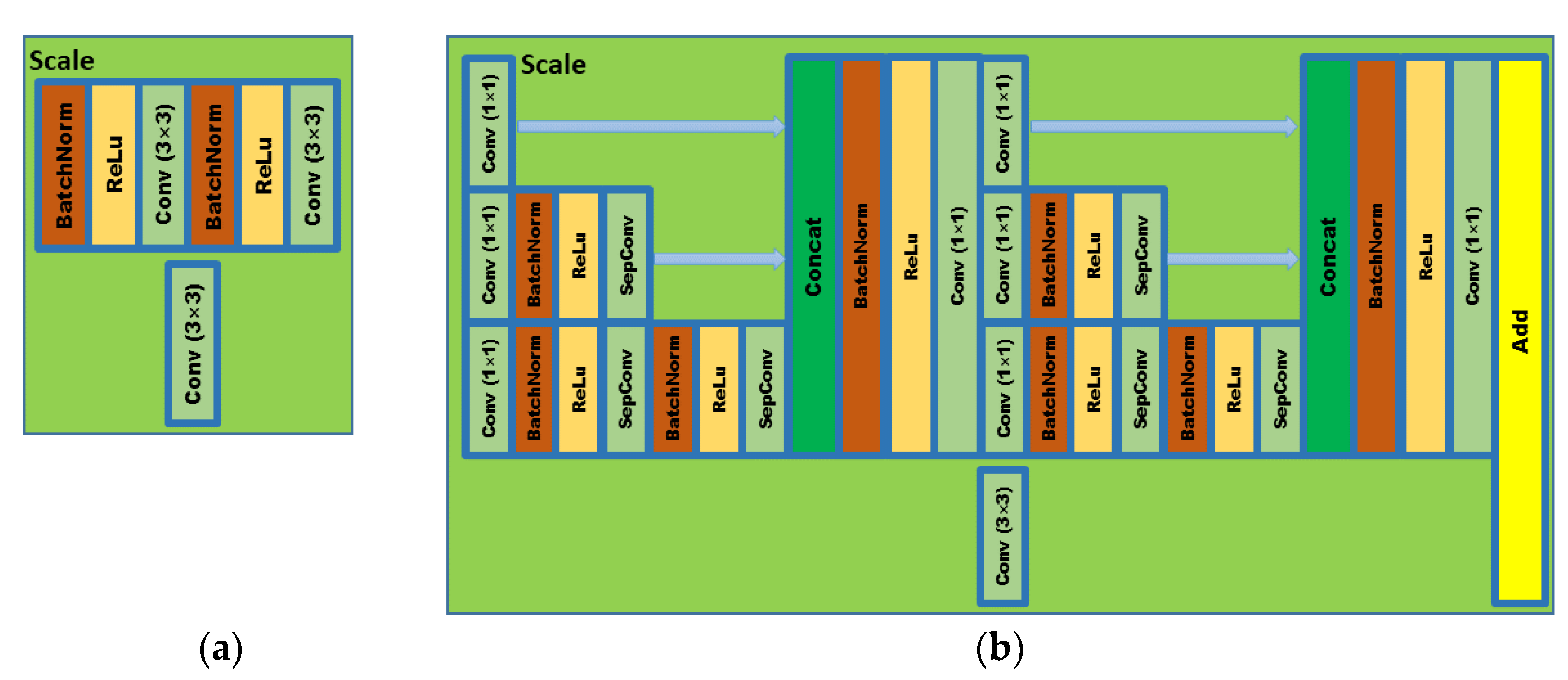
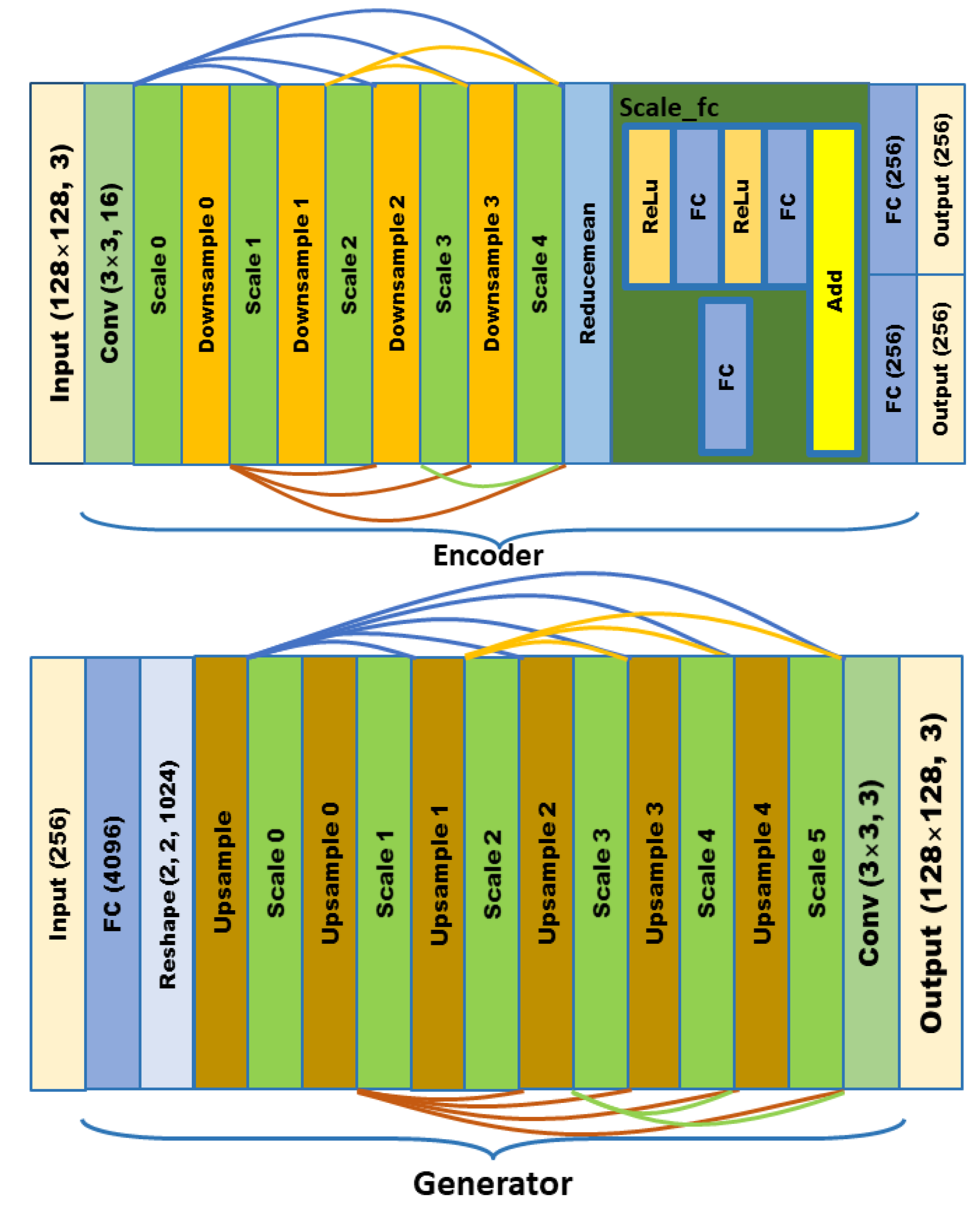
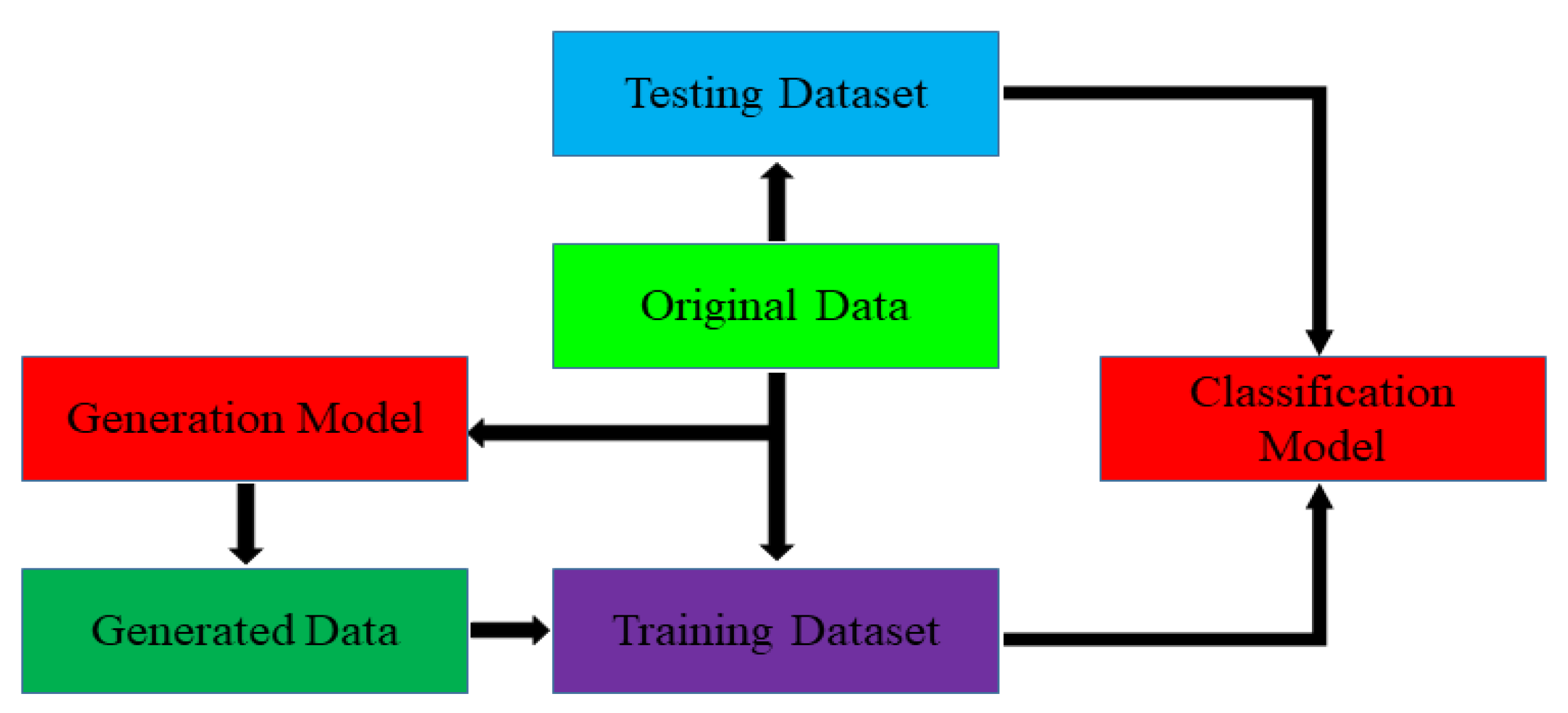
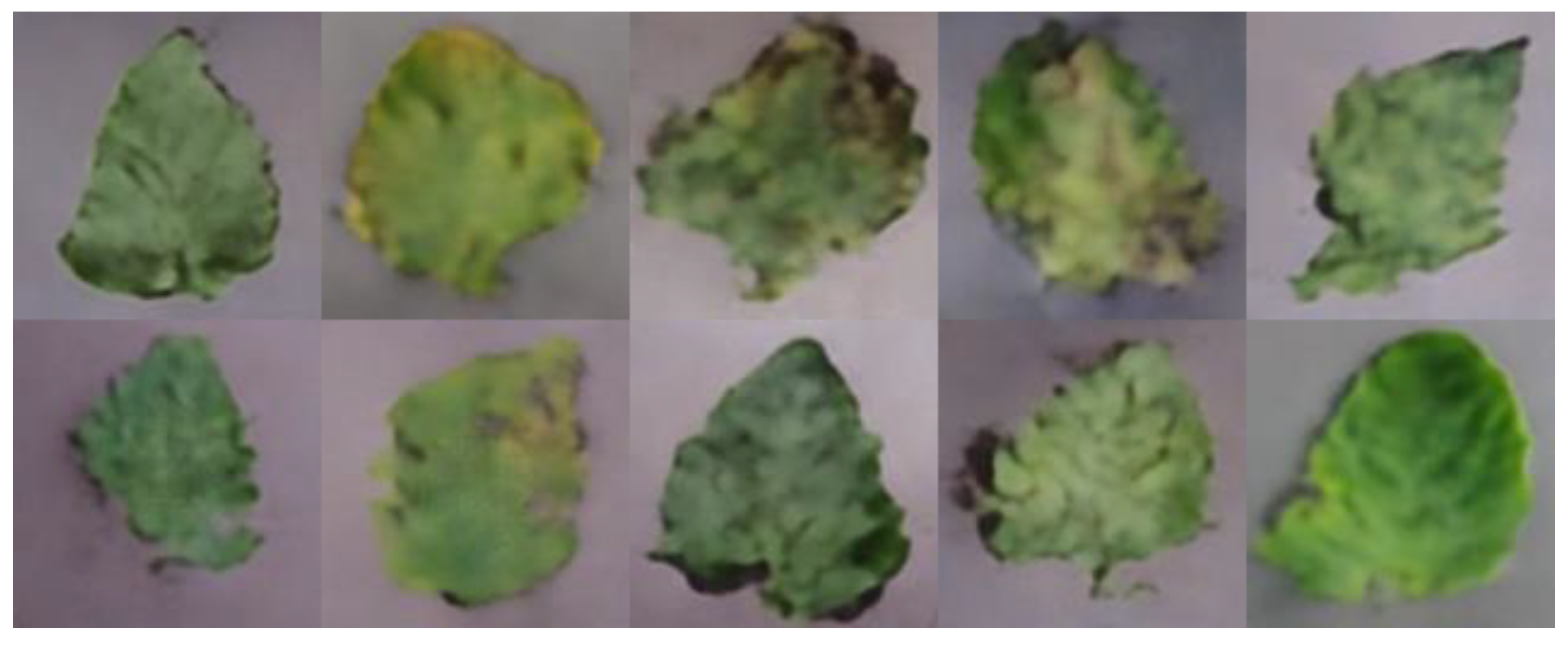
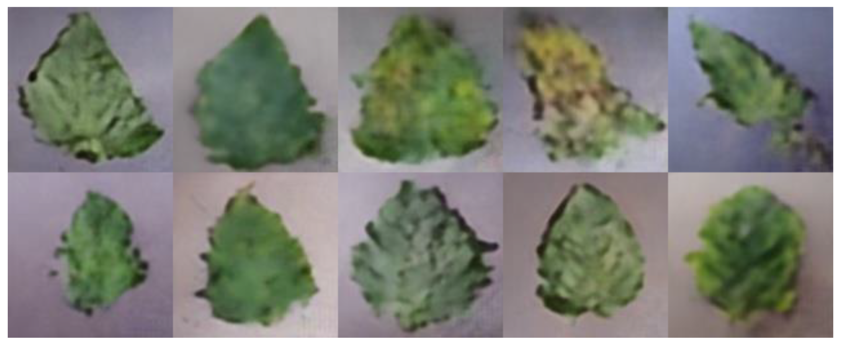
In order to meet the requirements of the training model for the large amount of image data, this paper proposes an image data generation method based on the Adversarial-VAE network model, which expands the image of tomato leaf diseases to generate images of 10 different tomato leaves, overcomes the overfitting problem caused by insufficient training data faced by the identification model. First, the Adversarial-VAE model is designed to generate images of 10 tomato leaves. Then, in view of the obvious differences in the area occupied by the leaves in the dataset and the insufficient accuracy of the feature expression of the diseased leaves using a single-size convolution kernel, the multi-scale residual learning module is used to replace the single-size convolution kernels to enhance the feature extraction ability, and the dense connection strategy is integrated into the Adversarial-VAE model to further enhance the image generative ability. The experimental results show that the tomato leaf disease images generated by Adversarial-VAE have higher quality than InfoGAN, WAE, VAE, and VAE-GAN on the FID. This method provides a solution for data enhancement of tomato leaf disease images and sufficient and high-quality tomato leaf images for different training models, improves the identification accuracy of tomato leaf disease images, and can be used in identifying similar crop leaf diseases.

The rest of the paper is organized as follows: Section 2 introduces the related work. Section 3 introduces the data enhancement methods based on Adversarial-VAE in detail and the detailed structure of the model. In Section 4, the experiment result is described, and the results are analyzed. Finally, Section 5 summarizes the article.

2. Related Work

2.1. Generative Adversarial Network (GAN)

The basic principle of GAN [16] is to obtain the probability distribution of the generator, making the probability distribution of the generator as similar as possible to the probability distribution of the initial dataset, including the generator and discriminator. The generator maps random data to the target probability distribution. In order to simulate the original data distribution as realistically as possible, the target generator should minimize the divergence between the generated data and the real data. Under real conditions, since the data set cannot contain all the information, GAN’s generator model cannot fit the probability distribution of the dataset well in practice, and the noise close to the real data is always introduced, so that new information will be generated. In reality, because the dataset cannot contain all the information, the GAN generator model cannot fit the probability distribution of the dataset well in practice, and it will always introduce noise close to the real data, which will generate new information. Therefore, the generated images are allowed to be used as data enhancement for further improving the accuracy of identification. The disadvantage of using GAN to generate images is it uses the random Gaussian noise to generate images, which means that it is not possible to generate any specified type of image. There is no way to decide which random noise can be used to generate the desired image, unless all the initial distribution can be tried. The generator network distinguishes between “real” and “fake” images through a confrontation process. However, the images obtained in this way are only as real as possible, but this does not guarantee that the content of the images is desired. In other words, it is possible that the generator network generates background images to make it as true as possible, but in fact, there is no real target in it.

2.2. Variational Auto-Encoder (VAE)

Variational auto-encoder (VAE) is an important generative model, which was proposed by Diederik P. Kingma and Max Welling [17], including two parts: encoder and decoder.

Figure 1 is the composition model of VAE. The data we can observe is $X$, and $X$ is generated by the latent variable $z$; and $z\to X$ is the generator model from the perspective of the auto-encoder. It is the decoder, and $X\to z$ is the recognition model, which is similar to the encoder of the auto-encoder. VAE is now widely used to generate images. When the generation model is trained, we can use it to generate images. Unlike GAN, the probability density function (PDF) of the image is known, while GAN does not know the image distribution. Using the auto-encoder can obtain the encoding distribution of such images through the encoding process of the output images, which is equivalent to knowing the corresponding noise distribution to each image, and then the desired image can be generated by selecting specific noise. When generating a new image, you only need to give the model a random implicit vector with a standard normal distribution, so that the desired image can be generated through the decoder, without the need to encode an original image first. In practice, it is necessary to make a trade-off between the accuracy of the model and the factor that the implicit vector obeys the standard normal distribution. The accuracy of the model refers to the degree of similarity between the image generated by the decoder and the original image.

2.3. VAE-GAN

VAE-GAN [23] adds a discriminator to the original VAE. If you just operate VAE, the image will be very blurred. After adding the discriminator, the output is forced to be as real as possible. From the perspective of GAN, when training GAN, the generator has never seen what the real image looks like. From the auto-encoder, the generator does not have to cheat the discriminator and has seen what the real image looks like. If you first pass the auto-encoder architecture and the generator has seen a real image, the VAE-GAN will be more stable to learn. VAE-GAN consists of the encoder, generator, and discriminator. The encoder is used to encode, that is, to convert the input image into a vector. The generator is the decoder in VAE, which converts the vector into an output image. Since it is hoped that the output after encoding and decoding is still itself, the input image and output image should be the same as much as possible. The discriminator is used to judge whether the image is realistic or fake (generated by the generator), and gives a scalar (score or probability or binary classification result). The goal of the combination of the encoder and generator is to keep an image as it is after encoding and decoding. Therefore, the updating criterion of the encoder is to minimize the variance of the image before the encoder and after the decoder, and to make the distribution of the image before the encoder and after the decoder as consistent as possible (the distribution is described by KL divergence). The updating criterion of the generator is to minimize the variance of images before the encoder and after the decoder, and the scores of generated and reconstructed images after the discriminator are also as high as possible. The updating criterion of the discriminator is to try to distinguish between the generated, reconstructed, and realistic images, so the scores for the original images are as high as possible, and the scores for the generated and reconstructed images should be as low as possible.

2.4. Two-Stage VAE

VAE is one of the most popular generation models, but the quality of the generation is relatively poor. The gaussian hypothesis of encoders and decoders is generally considered to be one of the reasons for the poor quality of the generation. The authors of [22] carefully analyzed the properties of the VAE objective function, and came to the conclusion that the encoder and decoder gaussian hypothesis of VAE does not affect the global optimal solution. The use of other more complex forms does not obtain a better global optimal solution.

According to [22], VAE can reconstruct training data well but cannot generate new samples well. VAE can learn the manifold where the data is, but the specific distribution in the manifold it learned is different from the real distribution. In other words, every data from the manifold will be perfectly reconstructed after VAE. For this reason, the first VAE is used to learn the position of the manifold, and the second VAE is used to learn the specific distribution within the manifold. Specifically, the first VAE transforms the training data into a certain distribution in the hidden space, which occupies the entire hidden space instead of on the low-dimensional manifold. The second VAE is used to learn the distribution in the hidden space since the latent variable occupies the entire hidden space dimension. Therefore, according to the theory, the second VAE can learn the distribution in the hidden space of the first VAE.

3. Materials and Methods

3.1. Dataset

PlantVillage [24] is an internet public image library of plant leaf diseases initiated and established by David, an epidemiologist at the University of Pennsylvania. This dataset collects more than 50,000 images of 14 species of plants with 38 category labels. Among them, 18,162 tomato leaves of 10 categories, which are respectively healthy leaves and 9 kinds of diseased leaves, were used as the basic data set of crop disease images for the experiment. Figure 2 shows an example of 10 tomato leaves. In the practical application, the image size was changed to 128 × 128 pixels during preprocessing in order to reduce both the calculation and training time of model.

3.2. Adversarial-VAE Model for Generating Tomato Leaf Disease Images

The deep neural network has a large number of adjustable parameters, so it needs a large amount of labeled data to improve the generalization ability of the model. However, there has always been a data vacuum in agriculture, making it difficult to collect a lot of data. At the same time, it is also difficult to label all collected data accurately. Due to a lack of experience, it is difficult to judge whether the identification is accurate, so experienced experts are needed to accurately label the data. In order to meet the requirements of the training model for the large amount of image data, this paper proposes an image data generation method based on the Adversarial-VAE network model, which expands the tomato leaf disease images in the PlantVillage dataset, and overcomes the problem of over-fitting caused by insufficient training data faced by the identification model.

3.2.1. Adversarial-VAE Model

The Adversarial-VAE model of tomato leaf disease images consists of stage 1 and stage 2. Stage 1 is a VAE-GAN network, consisting of an encoder (E), generator (G), and discriminator (D). Stage 2 is a VAE network, consisting of an encoder (E) and decoder (D).

The detailed model of Adversarial-VAE is shown in Figure 3. In stage 1, the input images are encoded and decoded, and the discriminator is used to determine whether the images are real or fake to improve the model’s generation ability. The input to the model is an image $X$ of size 128 × 128 × 3, which is compressed into two vectors μ and σ with a size of 256 after passing through the encoder network, and then combined into a latent vector $z$ with a size of 256. After passing through the generator network, size expansion is realized to generate an image $\overline{X}$ with a size of 128 × 128 × 3. The input of the discriminator network is the original image $X$, generated image $\hat{X}$, and reconstructed image $\overline{X}$ to determine whether the image is real or fake. Stage 2 encodes and decodes the latent variable $z$. Specifically, stage 1 transforms the training data $X$ into some distribution $z$ in the latent space, which occupies the whole latent space rather than on the low-dimensional manifold of the latent space. Stage 2 is used to learn the distribution in the latent space. Since latent variables occupy the whole dimension, according to the theory [22], stage 2 can learn the distribution in the latent space of stage 1. After the Adversarial-VAE model is trained, $z$ is sampled from the gaussian model and $\overline{z}$ is obtained through stage 2. $\overline{z}$ is obtained through the generator network of stage 1 to obtain $\hat{X}$, which is the generated sample and is used to expand the training set in the subsequent identification model.

3.2.2. Components of Stage 1

Stage 1 is a VAE-GAN network composed of an encoder (E), generator (G), and discriminator (D). It is used to transform training data into a certain distribution in the hidden space, which occupies the entire hidden space rather than on the low-dimensional manifold. The encoder converts an input image $X$ of size 128 × 128 × 3 into two vectors of mean and variance of size 256. The detailed encoder network of stage 1 is shown in Figure 4 and the output sizes of every layer are shown in

Table 1. Output size of the layer in the encoder network.

Layer	Input	Conv	Scale 0	Downsample 0	Scale 1	Downsample 1
Size	128 × 128 × 3	128 × 128 × 16	128 × 128 × 16	64 × 64 × 32	64 × 64 × 32	32 × 32 × 64
Layer	……	Downsample 3	Scale 4	Reducemean	Scale_fc	FC
Size	……	8 × 8 × 256	8 × 8 × 256	256	256	256

. The encoder network consists of a series of convolution layers. It is composed of Conv, 4 layers, Scale, Reducemean, Scale_fc and FC. The 4 layers is made up of four alternating Scale and Downsample, and Scale is the ResNet module, which is used to extract features. Downsample is used to decrease the size of each feather map and increase the number of channels. After each layer, the number of channels is doubled and the size is halved. The input of the model is a 128 × 128 × 3 image, the size of the input vector is changed to 128 × 128 × 16 after Conv layer, while after 4 layers, the size is 8 × 8 × 256. Reducemean is global pooling, and the structure of Scale_fc is shown in Figure 4 for better access to global information.

The generator is both VAE’s decoder and GAN’s generator, and they have the same function: converting vector to $\overline{X}$. The decoder is used to decode, restoring the latent vector $z$ of size 256 to an image of size 128 × 128 × 3. The goal of the combination of the encoder and generator is to keep an image as original as possible after the encoder and generator. The detailed generator network of stage 1 is shown in Figure 5 and related parameters are shown in

Table 2. Output size of the layer in the generator network.

Layer	Input	FC	Reshape	Upsample 0	Scale 0	Upsample 1
Size	256	4096	2 × 2 × 1024	4 × 4 × 512	4 × 4 × 512	8 × 8 × 256
Layer	……	Upsample 4	Scale 4	Upsample 5	Scale 5	Conv
Size	……	64 × 64 × 32	64 × 64 × 32	128 × 128 × 16	128 × 128 × 16	128 × 128 × 3

. The generator network consists of a series of deconvolution layers, which is composed of FC, 6 layers, and Conv. FC means fully connected. The input of the model is a vector with 256, which is drawn from a gaussian distribution or reparameterization from the output of the encoder network. The size is changed to 4096 after FC and to 2 × 2 × 1024 after Reshape further. Six layers are made up of six alternating Upsample and Scale. Upsample is deconvolution layer, which is used to expand the size of the feature map and reduce the number of channels. After each Upsample, the length and width of the feature map are doubled, and the number of channels is halved. Scale is the Resnet module, which is used to extract features. After 6 layers, the size is changed to 128 × 128 × 3. Additionally, after Conv, the size is changed to 128 × 128 × 3, which is the same size as the input image.

The discriminator will be able to differentiate the generated, reconstructed, and realistic images as much as possible. Therefore, the score for the original image should be as high as possible, and the scores for the generated and reconstructed images should be as low as possible. Its structure is similar to that of the encoder, except that the final two FCs with a size of 256 are generated at the end and replaced with FC with a size of 1. The output is true or false, which is used to enhance the image generation ability of the network, making the generated image more like the real image. The details are shown in Figure 6 and related parameters are shown in

Table 3. Output size of the layer in the discriminator network.

Layer	Input	Conv	Scale 0	Downsample 0	Scale 1	Downsample 1
Size	128 × 128 × 3	128 × 128 × 16	128 × 128 × 16	64 × 64 × 32	64 × 64 × 32	32 × 32 × 64
Layer	……	Downsample 3	Scale 4	Reducemean	Scale_fc	FC
Size	……	8 × 8 × 256	8 × 8 × 256	256	256	1

.

3.2.3. Components of Stage 2

Stage 2 is a VAE network consisting of the encoder (E) and decoder (D), which is used to learn the distribution of hidden space in stage 1 since the latent variables occupy the entire latent space dimension. Both the encoder (E) and decoder (D) are composed of a fully connected layer. The structure is shown in Figure 7. The input of the model is a latent vector with size 256, which is drawn from a gaussian distribution.

3.3. Improved Adversarial-VAE Model

3.3.1. Multi-Scale Convolution

In the PlantVillage dataset, there are obvious differences in the area occupied by the leaves in the image, so the single-size convolution kernel is not accurate enough to check the feature expression of disease leaves. Therefore, in order to make the extracted features more abundant, a multi-scale convolution kernel is applied instead of a single-size convolution kernel to construct the residual learning module so that tomato disease identification can achieve a higher accuracy rate, as shown in Figure 8.

In order to utilize the multi-scale convolution kernel, the convolutional layer in the original residual learning module designed according to the Inception [25] structure, and the computational amount required for the 5 × 5 convolution kernel is relatively large to reduce the number of parameters and increase the calculation speed. During practical application, the 5 × 5 convolution kernel is replaced by two 3 × 3 convolution kernels, which does not allow the convolution layer to be extracted to different levels with different receptive fields.

Specifically, a single 3 × 3 convolution kernel (Conv (3 × 3)) in ResNet is replaced by multiple convolution kernels to expand the convolution width, and the information obtained from each convolution kernel is added up through Concat. After BatchNorm and Relu, the mixed feature of Conv (1 × 1) is used as the input of the next operation. Multiple convolution cores here refer to 1 × 1 convolution kernel (Conv (1 × 1)), 1 × 1 convolution (Conv (1 × 1)) followed by separable convolution (SepConv), and 1 × 1 convolution (Conv (1 × 1)) followed by separable convolution (SepConv) followed by separable convolution (SepConv). Depthwise convolutions are also used to construct a lightweight deep neural network. In this case, the standard convolution is decomposed into depthwise convolution and pointwise convolution. Each channel is convolution individually, which is used to combine the information of each channel to reduce model parameters and computation.

3.3.2. Dense Connection Strategy

As another CNN with a deeper number of layers, Densenet has fewer parameters than Resnet. Its bypass enhances the reuse of features, and the network is easier to train and has a certain regularization effect, and alleviates the problems of gradient vanishing and model degradation. The problem of gradient disappearance is more likely to occur when the network depth is deeper. The reason is that the input information and gradient information are transmitted between many layers. Now, dense connection is equivalent to each layer directly connecting input and loss, so the phenomenon of gradient disappearance can be reduced and the network depth can be increased. Therefore, the dense connection strategy from DenseNet [26] is applied to the encoder network and generator network in stage 1. Each layer uses the feature map as the input of the latter layer, which can effectively extract the features of the lesion and alleviate the disappearing gradient. As shown in Figure 9, due to the inconsistency of the feature scales of the front and back layers, 1 × 1 convolution is used to achieve the consistency of feature scales. The dense connection strategy shares the weights of the prior layers and improves the feature extraction capabilities.

3.4. Loss Function

Stage 1 is VAE-GAN network. In stage 1, the goal of the encoder and generator is to keep an image as original as possible after code. The goal of the discriminator is to try to differentiate the generated, reconstructed, and realistic images. The training pipeline of the stage 1 Algorithm 1 is as follows:

Algorithm 1: The training pipeline of the stage 1.

Initial parameters of the models: ${\theta }_e$$, {\theta }_g$$, {\theta }_d$

while training do

$x^{real}\leftarrow$ batch of images sampled from the dataset.

${z_{\mu }}^{real},{z_{\sigma }}^{real}\leftarrow E_{{\theta }_e}(x^{real})$

$z^{real}\leftarrow {z_{\mu }}^{real}+\epsilon {z_{\sigma }}^{real}$$\mathrm{with} \epsilon \sim N\left(0,Id\right)$

${\overline{x}}^{real}\leftarrow G_{{\theta }_g}(z^{real})$

$z^{fake}\leftarrow$$\mathrm{prior} P(z)$

$x^{fake}\leftarrow G_{{\theta }_g}(z^{fake})$

{Compute losses gradients and update parameters.}

${\theta }_e\overline{\leftarrow }\Vert {\overline{x}}^{real}-x^{real}\Vert +KL(P(z^{real}|x^{real})\Vert P(z))$

${\theta }_g\overline{\leftarrow }\Vert {\overline{x}}^{real}-x^{real}\Vert -D_{{\theta }_d}({\overline{x}}^{real})-D_{{\theta }_d}(x^{fake})$

${\theta }_d\overline{\leftarrow }{D}_{{\theta }_d}({\overline{x}}^{real})+D_{{\theta }_d}(x^{fake})-D_{{\theta }_d}(x^{real})$

end while

Stage 2 is the VAE network. In stage 2, the goal of the encoder and decoder is to keep an image as original as possible after codec. Therefore, the updating criterion of the encoder is to minimize the variance of the image before the encoder and after the decoder, and to make the distribution of the image as consistent as possible before the encoder and after the decoder. The updated criterion of the decoder is to minimize the variance of images before the encoder and after the decoder. The training pipeline of the stage 2 Algorithm 2 is as shown below:

Algorithm 2: The training pipeline of the stage 2.

Initial parameters of the models: ${\theta }_e$$, {\theta }_d$.

while training do

$z^{real}\leftarrow$ Gaussian distribution.

${u_{\mu }}^{real},{u_{\sigma }}^{real}\leftarrow E_{{\theta }_e}(z^{real})$.

$u^{real}\leftarrow {u_{\mu }}^{real}+{\epsilon u_{\sigma }}^{real}$$\mathrm{with} \epsilon \sim N\left(0,Id\right)$.

${\overline{z}}^{real}\leftarrow D_{{\theta }_d}(u^{real})$.

$u^{fake}\leftarrow$$\mathrm{prior} P(u)$.

$z^{fake}\leftarrow D_{{\theta }_d}(u^{fake})$.

{Compute losses gradients and update parameters.}

${\theta }_e\overline{\leftarrow }\Vert {\overline{z}}^{real}-z^{real}\Vert +KL(P(u^{real}|z^{real})\Vert P(u))$.

${\theta }_d\overline{\leftarrow }\Vert {\overline{z}}^{real}-z^{real}\Vert$.

end while

3.5. Experimental Setup

The experimental configuration environment of this paper is as follows: Ubuntu16.04 LST 64-bit system, processor Intel Core i5-8400 (2.80 GHz), memory is 8 GB, graphics card is GeForce GTX1060 (6G), and using the Tensorflow-GPU1.4 deep learning framework with python programming language.

3.6. Performance Evaluation Metrics

The FID evaluation model is introduced to evaluate the performance of the image generation task. The FID score was proposed by Martin Heusel [27] in 2017. It is a metric for evaluating the quality of the generated image and is specifically used to evaluate the performance of GAN. It is a measure of the distance between the feature vector of the real image and the generated image. This score is proposed as an improvement on the existing inception score (IS) [28,29]. It calculates the similarity of the generated image to the real image, which is better than the IS. The disadvantage of IS is that it does not use statistics from the true sample and compare them to statistics from the generated sample.

As with the IS, the FID score uses the Inception V3 model. Specifically, the coding layer of the model (the last pooled layer before the classified output of the image) is used to extract the features specified by computer vision techniques for the input image. These activation functions are calculated for a set of real and generated images. By calculating the mean value and covariance of the image, the output of the activation function is reduced to a multivariable gaussian distribution. These statistics are then used to calculate the real image and generate activation functions in the image collection. The FID is then used to calculate the distance between the two distributions. The lower the FID score, the better the image quality. On the contrary, the higher the score, the worse the quality.

4. Results and Discussion

In order to verify the effectiveness of the leaf disease identification model proposed in this paper, a total of 18,162 images of the tomato disease from PlantVillage are randomly divided into a training set, verification set, and test set, of which the training set accounts for about 60%, which means 10,892 images, as shown in

Table 4. Detailed information of the tomato leaf disease dataset.

Class	All Sample Numbers	60% of Sample Numbers
healthy	1592	954
TBS	2127	1276
TEB	1000	600
TLB	1910	1145
TLM	952	571
TMV	373	223
TSLS	1771	1062
TTS	1404	842
TTSSM	1676	1005
TYLCV	5357	3214
ALL	18,162	10,892

. The verification set accounts for about 20% or 3632 images, and the test set accounts for about 20% or 3636 images. They are used to train the model, select the model, and evaluate the performance of the proposed model.

The Adversarial-VAE model is used to generate training samples, and the number of generated samples is consistent with the number of samples corresponding to the original training set, so the sample size is doubled, and the generated data is added to the training set. For these datasets with generated images, all the generated images are placed in the training set, and all the images in the test set are from the initial dataset. The test set is completely derived from the initial dataset. The flowchart of the data augmentation method is shown in Figure 10. In the figure, generative model refers to the generation part of the Adversarial-VAE model, which is composed of stage 2 and the generator network in stage 1. After the Adversarial-VAE model is trained, $z$ is sampled from the Gaussian model, and $\overline{z}$ is obtained through stage 2, and $\overline{X}$ is obtained through the generator network of stage 1, which is the generated sample. For 10 kinds of tomato leaf images, we train 10 Adversarial-VAE models. For each class, we generate samples by sampling vectors corresponding to the number of categories from the gaussian model in order to generate a different number of samples.

4.1. Generation Results and Analysis

The proposed Adversarial-VAE networks are compared with several advanced generation methods, including InfoGAN, WAE, VAE, VAE-GAN, and 2VAE, which are used to generate tomato diseased leaf images. We compare the reconstructed image quality and the generated image quality through the FID score as shown in

Table 5. Reconstruction-FID comparison between different generative methods.

Reconstruction-FID	InfoGAN [19]	WAE [21]	VAE [17]	VAE-GAN [23]	2VAE [22]	Adversarial-VAE
healthy	172.61	129.47	155.64	130.08	155.64	130.08
TBS	135.29	103.11	148.07	114.24	148.07	114.24
TEB	126.96	106.69	138.87	100.59	138.87	100.59
TLB	180.10	111.81	169.80	119.23	169.80	119.23
TLM	160.93	133.79	161.37	147.08	161.37	147.08
TMV	144.71	125.86	157.20	140.23	157.20	140.23
TSLS	120.24	90.43	139.41	108.57	139.41	108.57
TTS	107.88	81.74	137.89	99.67	137.89	99.67
TTSSM	114.22	91.23	141.42	106.89	141.42	106.89
TYLCV	140.11	83.23	133.05	79.76	133.05	79.76
AVERAGE	140.31	105.74	148.27	114.63	148.27	114.63

and

Table 6. Generation-FID comparison between different generative methods.

Generation-FID	InfoGAN [19]	WAE [21]	VAE [17]	VAE-GAN [23]	2VAE [22]	Adversarial-VAE
healthy	221.86	202.06	186.37	167.46	179.83	162.57
TBS	232.88	221.85	190.71	178.75	187.09	179.96
TEB	183.09	169.42	158.43	132.42	153.65	133.65
TLB	277.65	227.51	192.38	184.64	199.17	180.71
TLM	235.07	219.42	200.15	200.90	196.47	197.45
TMV	210.91	211.38	191.24	214.60	196.78	210.54
TSLS	199.31	182.59	156.61	148.31	152.93	146.11
TTS	199.87	208.23	191.90	163.99	185.01	161.07
TTSSM	195.08	210.70	175.97	147.95	173.95	146.83
TYLCV	182.74	172.82	151.22	99.60	146.89	98.76
AVERAGE	213.85	202.60	179.50	163.86	177.18	161.77

. Table 5 lists the FID of the reconstruction images under the different neural network models. Table 6 shows the FID comparison between different generative methods. Reconstruction-FID demonstrates the ability of this method to reconstruct the original input image. The lower the value is, the better the reconstruction capability is. Generation-FID demonstrates the ability of this method to generate new images. The lower the value is, the better the reconstruction capability is.

Table 5 and Table 6 show Reconstruction-FID and Generation-FID of 10 kinds of tomato leaf images, respectively. From the tables, we can see that WAE is better at reconstruction of the images than other methods. The average FID score is 105.74, which is the lowest score, and it also obtained the lowest score in most categories except TBS and TYLCV, which means WAE has excellent ability in reconstruction. Adversarial-VAE is the best in the generation of the images. The average FID score is 161.77, which is the lowest score, and it also obtained the lowest score in most categories, which means Adversarial-VAE has more advantages in generation than the others.

Generation-FID of Adversarial-VAE alone, Adversarial-VAE + multi-scale convolution, Adversarial-VAE + dense connection strategy, and the improved Adversarial-VAE, which used multi-scale convolution and the dense connection strategy, are compared in

Table 7. Generation-FID comparison of the proposed generative method.

Generation-FID	Adversarial-VAE Alone	Adversarial-VAE + Multi-Scale Convolution	Adversarial-VAE + Dense Connection Strategy	Improved Adversarial-VAE
healthy	162.57	162.64	167.63	171.63
TBS	179.96	170.29	176.3	167.53
TEB	133.65	128.28	130.81	126.84
TLB	180.71	175.15	170.42	166.92
TLM	197.45	194.81	191.42	187.79
TMV	210.54	202.39	198.28	189.09
TSLS	146.11	151.91	147.11	151.8
TTS	161.07	155.89	166.72	165.84
TTSSM	146.83	144.54	143.74	142.32
TYLCV	98.76	98.31	98.64	99.79
AVERAGE	161.77	158.42	159.11	156.96

. The average FID score is 156.96, which is the lowest score, and it also obtained the lowest score in most categories. As can be seen from the table, the improved model reduced the FID score for most types of disease, with an average FID score reduction of 4.81. It shows that the improved model has a better generative ability. The generated images are shown in Figure 11 based on Adversarial-VAE. And Figure 12 shows the generated images based on VAE networks.

4.2. Identification Results and Analysis

The original training set contains 10,892 images. After using improved Adversarial-VAE, the training set is expanded to 21,784 images. For comparative experiments, the original data set is expanded twice by replication, namely 21,784 images. Three experiments are carried out to train the classification network as shown in Figure 13 to identify tomato leaf diseases. During the operation, the training set and the test set are divided into batches by batch training. The batch training method is used to divide the training set and the test set into multiple batches. Each batch trains 32 images, that is, the minibatch is set to 32. After training 4096 images, the verification set is used to determine the retained model. After training all the training set images, the test set is tested. Each test batch is set to 32. All the images in a training set are iterated through as an iteration (epoch) for a total of 10 iterations. The model is optimized in using the momentum optimization algorithm and the learning rate is set at 0.001.

Table 8. Classification accuracy of the classification network trained with the expanded training set generated by different generative methods.

	Classification Alone	InfoGAN + Classification	WAE + Classification	VAE + Classification	VAE-GAN + Classification	2VAE + Classification	Improved Adversarial-VAE + Classification
Accuracy	82.87%	82.42%	82.16%	84.65%	86.86%	85.43%	88.43%

shows the classification accuracy of the classification network trained with the expanded training set generated by different generative methods. After training the classification network with the original training set, the identification accuracy on the test set is 82.87%; With the double original training set, the identification accuracy on the test set is 82.95%, and after training the classification network with the training set expanded by improved Adversarial-VAE, the identification accuracy reaches 88.43%, an increase of 5.56%. Compared with the double original training set, it also improved by 5.48%, which proves the effectiveness of the data expansion. The InfoGAN and WAE generative models were used to generate samples for the training the classification network, but the classification accuracy was not improved, which can be understood as poor sample generation and no effect was mentioned for training, as shown in Table 8.

5. Conclusions

Leaf disease identification is the key to control the spread of disease and ensure healthy development of the tomato industry. The deep neural network-based method requires a lot of data for training. However, there is little data in many agricultural fields. In the field of tomato leaf disease identification, it is a waste of manpower and time to collect large-scale labeled data. Labeling of training data requires very professional knowledge. All these factors lead to either the number and category of labeling being relatively small, or the labeling data for a certain category being very small, and manual labeling is very subjective work, which makes it difficult to ensure high accuracy of the labeled data.

To solve the problem of a lack of training images of tomato leaf diseases, an Adversarial-VAE network model was proposed to generate images of 10 different tomato leaf diseases to train the recognition model. Firstly, an Adversarial-VAE model was designed to generate tomato leaf disease images. Then, the multi-scale residuals learning module was used to replace the single-size convolution kernel to enhance the ability of feature extraction, and the dense connection strategy was integrated into the Adversarial-VAE model to further enhance the ability of image generation. The Adversarial-VAE model was only used to generate training data for the recognition model. During the training and testing phase of the recognition model, no computation and storage costs were introduced in the actual model deployment and production environment. A total of 10,892 tomato leaf disease images were used in the Adversarial-VAE model, and 21,784 tomato leaf disease images were finally generated. The image of tomato leaf diseases based on the Adversarial-VAE model was superior to the InfoGAN, WAE, VAE, and VAE-GAN methods in FID. The experimental results show that the proposed Adversarial-VAE model can generate enough of the tomato plant disease image, and image data for tomato leaf disease extension provides a feasible solution. Using the Adversarial-VAE extension data sets is better than using other data expansion methods, and it can effectively improve the identification accuracy, and can be generalized in identifying similar crop leaf diseases. In future work, in order to improve the robustness and accuracy of identification, we will continue to find better data enhancement methods to solve the problem of tomato leaf disease identification, which can be applied to the detection networks.

This method was proposed based on improving the classification accuracy on the basis of many labeled samples. At the beginning of this study, the most direct way was to expand each class with one network, so that when new categories need to be added, only one network needs to be trained with the samples of the new category, instead of retraining with all samples. We also considered training only one network to generate data samples of different categories by adding an input as a category control, but this has the side effect of requiring several networks to be retrained if new categories need to be generated. If there is no large amount of annotated data as training samples for training the generative model, for example, disease leaves for another plant cannot cover the sample space, the generative model cannot be directly trained in this way, and the number of samples needs to be expanded first. In practice, it is difficult to collect disease leaf images, so the problem of few-shot learning needs to be solved urgently. In summary, we will strive to achieve continuous improvement of the performance and try to apply it to practical agricultural production.