Development of a Low-Cost Semantic Monitoring System for Vineyards Using Autonomous Robots

Abstract

Many tasks involved in viticulture are labor intensive. Farmers frequently monitor the vineyard to check grape conditions, damage due to infections from pests and insects, grape growth, and to estimate optimal harvest time. Such monitoring is often done manually by the farmers. Manual monitoring of large vineyards is time and labor consuming process. To this end, robots have a big potential to increase productivity in farms by automating various tasks. We propose a low-cost semantic monitoring system for vineyards using autonomous robots. The system uses inexpensive cameras, processing boards, and sensors to remotely provide timely information to the farmers on their computer and smart phone. Unlike traditional systems, the proposed system logs data ‘semantically’, which enables pin-pointed monitoring of vineyards. In other words, the farmers can monitor only specific areas of the vineyard as desired. The proposed algorithm is robust for occlusions, and intelligently logs image data based on the movement of the robot. The proposed system was tested in actual vineyards with real robots. Due to its compactness and portability, the proposed system can be used as an extension in conjunction with already existing autonomous robot systems used in vineyards. The results show that pin-pointed remote monitoring of desired areas of the vineyard is a very useful and inexpensive tool for the farmers to save a lot of time and labor.

1. Introduction

Viticulture, a branch of horticulture, is the cultivation and harvesting of grapes and is carried out in many countries. The tasks involved in viticulture include monitoring, irrigation, adding fertilizers, canopy management, controlling pests and diseases, monitoring fruit development and characteristics, deciding the harvesting time, and vine pruning during the winter months. Among these, tasks such as harvesting and vine pruning are performed at specific times. The task of irrigating the vineyard is simple to automate. However, monitoring fruit development and characteristics is typically carried out frequently over the entire area of the vineyard, and is a labor intensive and time consuming task as it involves visual inspection of the fruit and plants by the farmer.

Frequent monitoring of the crop is important to check for pests and diseases in leaves and grapes, to check the growth of grapes, and to inspect for any damage. Typical estimation of optimal harvest time is also done visually and may vary for different types of grapes in different areas. Monitoring of humidity levels and mineral levels in the soil, temperature, etc. is done by directly embedding sensors in the soil and various IoT approaches have been proposed [1,2,3,4,5,6,7,8,9]. However, visual inspection of crop is another key aspect of monitoring. Visual monitoring is important for a viticulturist and involves the following key features:

• Grape growth: A viticulturist generally inspects the growth of grapes visually.
• Damage inspection: During the flowering of vine, strong winds and hail can cause damage. Cold temperatures may cause millerandage producing clusters with varying sizes or no seeds [10]. On the other hand, hot conditions may cause coulure causing grape clusters to either drop or not develop fully. This monitoring is often performed visually.
• Oidium inspection: Oidium is a fungal disease which has the potential to attack all the green parts of the vine with devastating consequences [11]. This is inspected visually.
• Peronospora inspection: Peronospora are obligate plant pathogens producing a downy mildew disease, which in turn produces stains on leaves [12]. Its treatment involves spraying copper sulphate [13]. This can be inspected visually at an early stage.
• Phylloxera inspection: Phylloxera [14] is a pest of commercial grapevines worldwide and can easily be inspected visually.
• Monitoring for green harvest: Green harvesting is the process in which immature and green grape bunches are purposefully removed so that the vine uses all the nutrients for developing the remaining grapes. This helps to develop and ripen the grape with good flavors.
• Estimation of harvest time and areas: Visual monitoring is important to estimate the appropriate harvest time and areas of the vineyard.
• Yield estimation: Visual estimation is important to estimate an approximate yield estimation of a vineyard.

Thus, visual monitoring of vineyard is crucial with many advantages. However, manual monitoring is a labor and time consuming task.

The present work was conducted in Japan, which prominently grows around 30–40 varieties of grapes, each with its own unique taste and fragrance [15]. Worth mentioning among these are: the Kyoho variety, which is also known as the king of grapes and popular for its juiciness and plump; the Muscat of Alexandria; the small seedless Delaware; and the Pione, famous for its flavor [15,16]. Almost all areas except the Nansei Islands are suitable for grapes, so grapes are produced in a wide range from Hokkaido to Kyushu prefectures of Japan. In Japan, nearly 90% of produced grapes are used for raw food, whereas less than 10% of the produced grapes are used for processing wine, grape juice, confectionery, etc. Japan does not export grapes but around 10,000 tons of grapes are imported annually [17]. The most cultivated variety in Japan is Kyoho, which is cultivated on 5465 ha. Delaware follows with 2967 ha, Pione with 2430 ha, and Campbell Early with 655 ha [18].

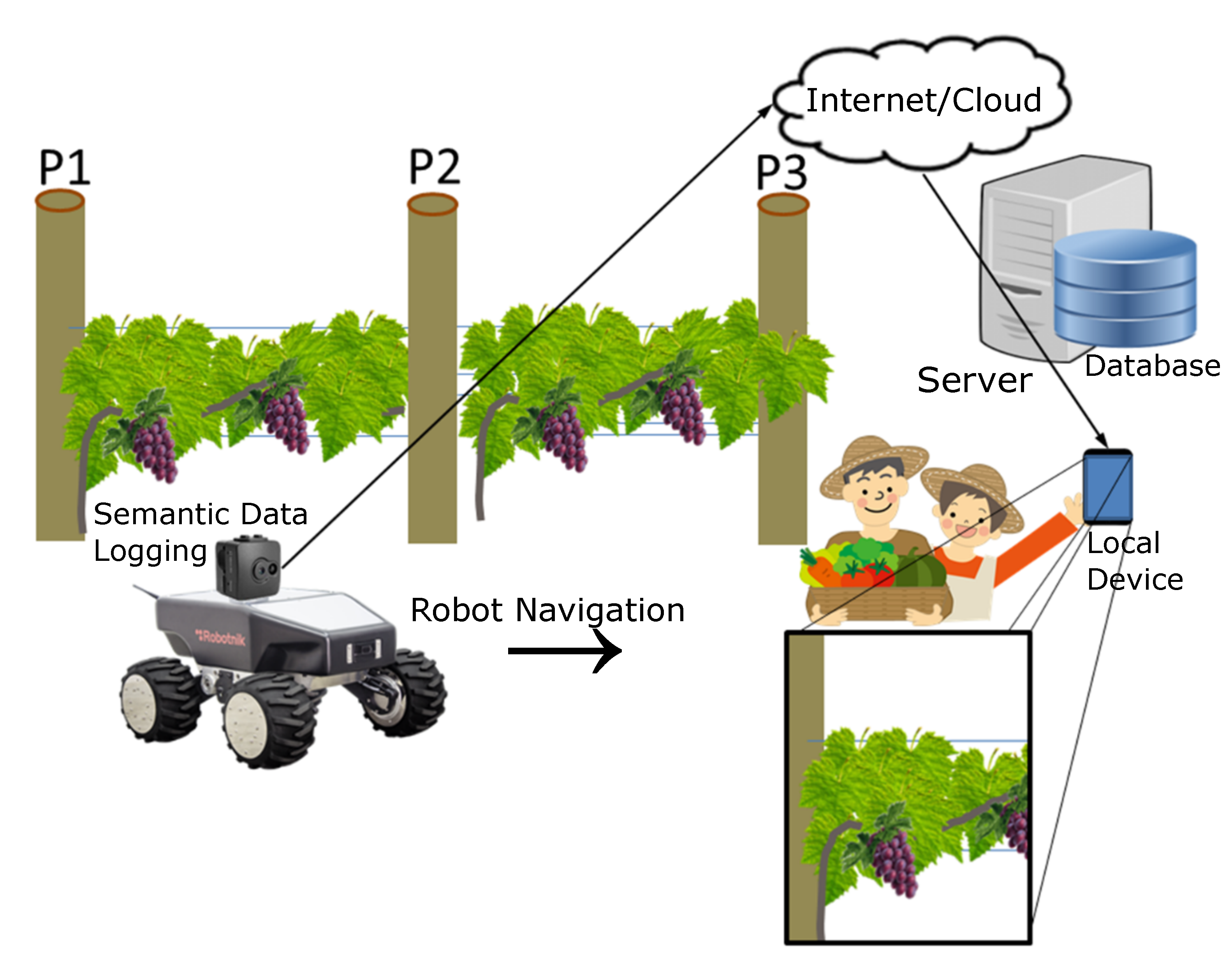
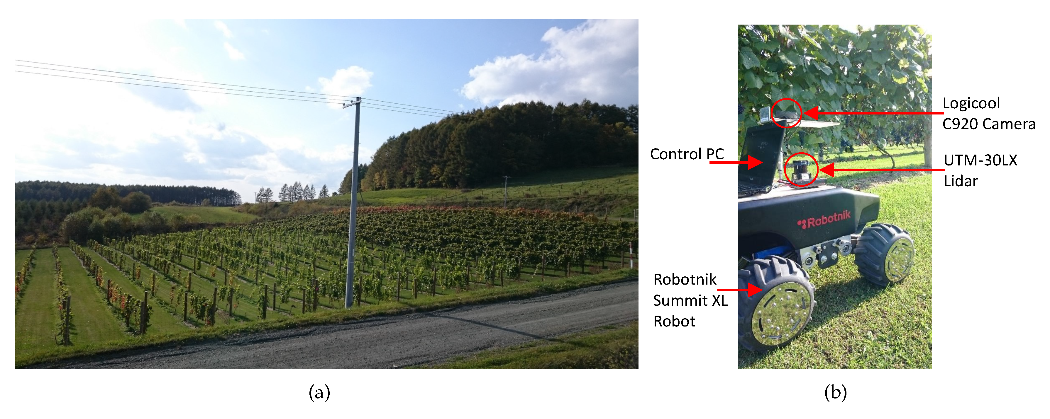
There are different varieties of grapes, and the practice of viticulture varies from place to place. In Japan, vineyards are located in hilly regions and generally characterized by cultivating grape plants in a nearly straight line. Grapevines are climbing plants that do not have their own natural support as with trees; hence, the grape plants are supported between wooden pillars which are called trunks. The grape plants grow to a certain height and hang on the supporting wires or rope above a certain distance from the ground. Hence, the pillars can serve as concrete features in the vineyards.

The focus of the proposed work is on visual monitoring using autonomous robots. Autonomous robots have successfully been employed in construction, manufacturing, and many aspects of agriculture industry. The motivation behind the proposed work lies in reducing the labor of farmers and bringing efficiency in grape production through the use of autonomous robots.

Recently, significant works related to autonomous vineyard robots have been proposed for different purposes. Some researchers have focused on localization of the robots, while others have focused on trunk recognition for single- [19,20] and multi-robot scenarios [21]. Apart from these, researchers have also focused on the problems of autonomous pruning [22], irrigation [23], yield estimation [24,25], and skeletonization [26] in vineyards by using autonomous robots. Color image-based grape detection is proposed in [27]. In [28], a monitoring robot for mountain vineyards is proposed. Mapping and localization in vineyard is discussed in [29]. Researchers have also focused on the improvement of plague control tasks, specifically on the distribution and placement of pheromone dispensers for matting disruption in the vineyards in [30]. Precision agriculture using multi-rotor micro aerial vehicles and human-carried multi-spectral 3D imaging device is proposed for automated monitoring in [31]. Wireless sensor network for vineyard monitoring that uses image processing is proposed in [32]. Other projects (e.g., Vinbot [33]) are also worth mentioning.

The novel contributions of this paper are summarized below:

• A vineyard monitoring system which only uses inexpensive camera sensor is proposed.
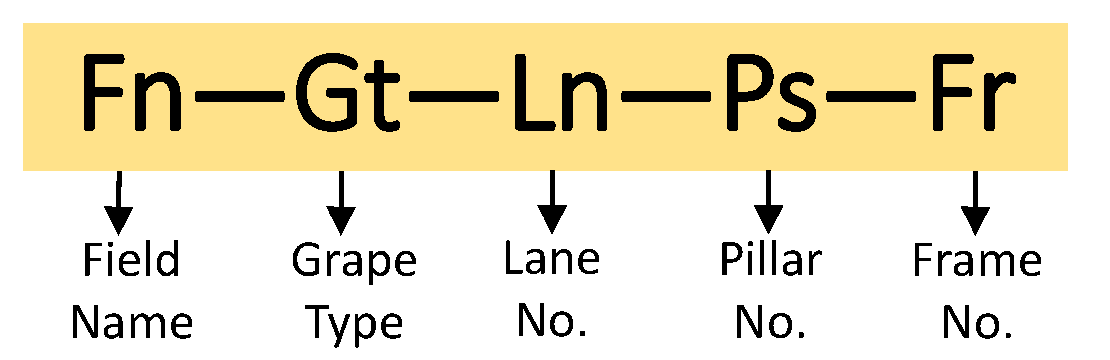
• We propose a novel way to semantically label image data in vineyards by detecting the pillars set in the vineyard to support grapes. The system labels the image data on the basis of field name, lane number, and pillar numbers, which are automatically identified through image processing. Unlike traditional monitoring techniques, the proposed semantic labeling enables pin-point monitoring of the vineyard. In other words, farmers do not need to access the whole data, but instead can specify the exact location in the field which needs to be monitored. This is very efficient and time saving. Feature detection is important for semantic labeling. While extracting features such as walls, corners, and straight lines are easier in indoor environments, robust feature extraction in vineyard is difficult due to the dynamic nature of the environment (viz. moving leaves, plant’s trunk, changing lighting conditions, etc.). Hence, robust feature extraction is a major challenge faced by mobile robots in farms, which generally lack static features. Due to this, many researchers tend to use expensive sensors such as GPS, dense RGBD sensors, and 3D Lidar (e.g., VLP-16/32), or sensor networks [34,35,36]. However, such sensors increase the system cost. Feature detection is done using inexpensive cameras in the proposed research.
• A way to increase the robustness of the system by varying the range of detection is proposed.
• An algorithm to automatically turn data logging on and off has been proposed based on the motion of robot.
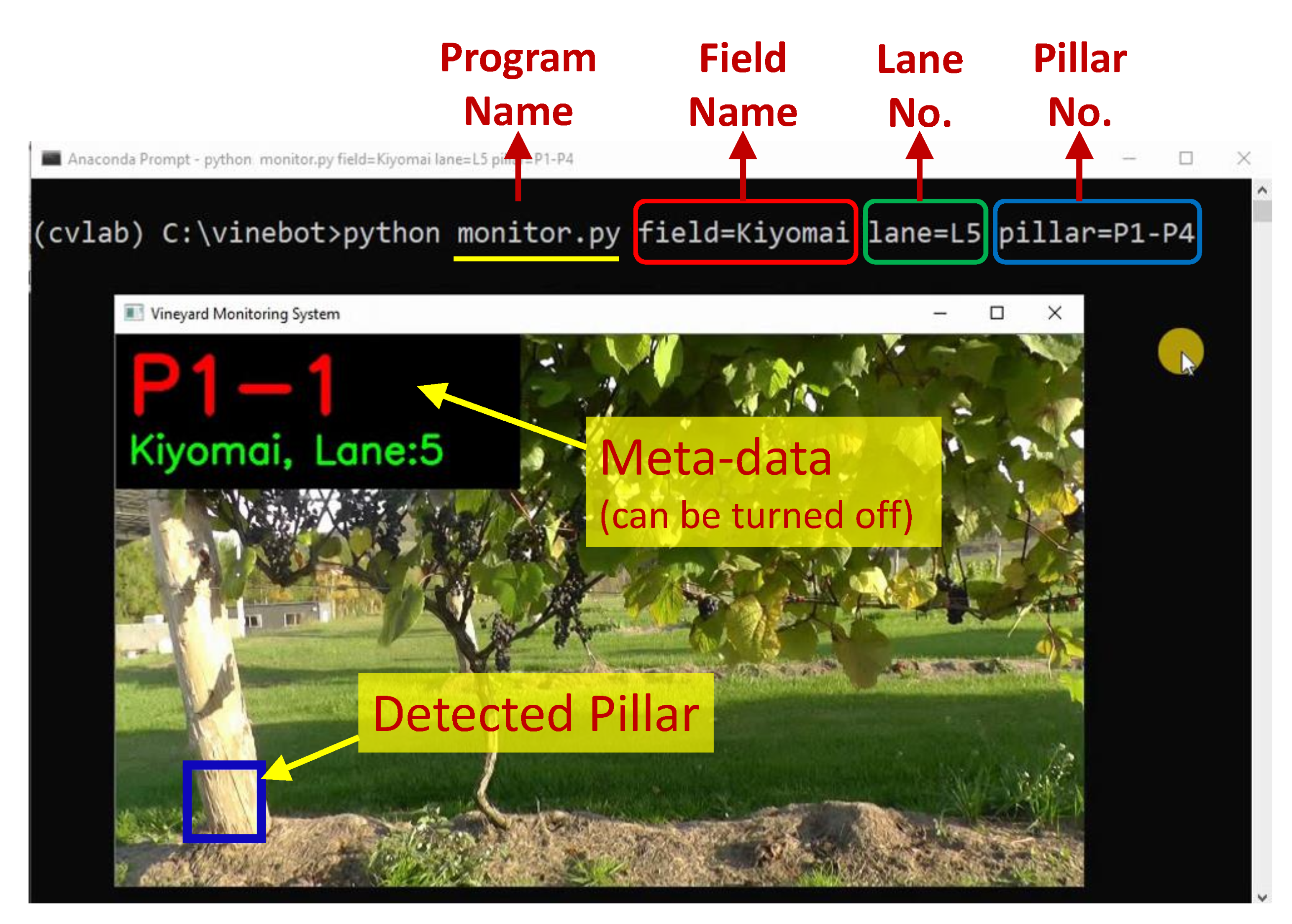
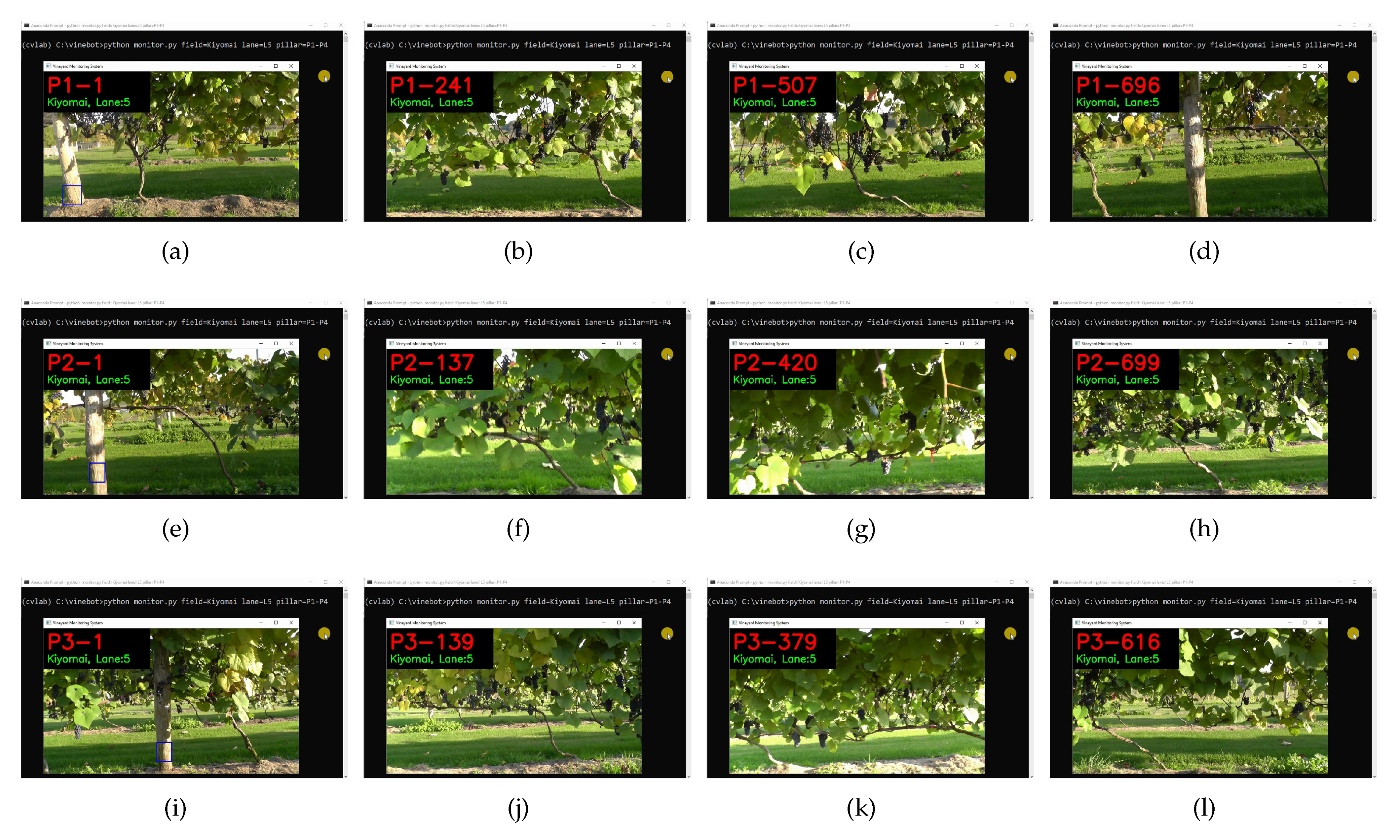
• An interactive software has been developed through which the farmers can monitor the vineyard.

The rest of the paper is organized as follows. Section 2 explains the main idea and system overview. Section 3 explains the landmark (pillar) detection algorithm, which forms the basis of semantic data labeling. Section 4 shows how the robustness of landmark detection algorithm is improved without significantly impacting the processing time. Semantic data logging is explained in Section 5. Section 6 discusses experimental results in real environments with actual robots. Section 6.1 shows the results of pillar detection in actual vineyard. Section 6.2 discusses the processing time. Section 6.3 explains about the monitoring software to interactively monitor the vineyard on a pin-point basis. Finally, Section 7 concludes the paper.

2. System Overview

Figure 1 shows the overview of the proposed semantic monitoring system. The monitoring system comprises of a camera with a processing board. The system is set on the top of an autonomous robot with the camera facing the grapes. In other words, the camera is setup perpendicular to the direction of motion of the robot. As the robot navigates the vineyard, the camera records the images in its local database. The images are processed and pillars are detected in the field. These pillars are shown as $\mathrm{P}1,\mathrm{P}2,\cdots \mathrm{P}3$ in Figure 1.

The robot localizes itself in the field using a Simultaneous Localization and Mapping (SLAM) module [37,38,39]. The robot identifies the field name, lane number, and pillar numbers using image processing and labels the image data with this information. Semantic data are thus logged and stored in the robot’s database. These data are then uploaded to a remote server. Farmers can access this information on their smart-phone, tablet-PC, or computer using a monitoring software which has been developed. Farmers can monitor the entire vineyard from their home. They can also pinpoint the areas they want to monitor. Moreover, they can compare a particular location with the past data. Farmers can thus monitor the growth of grapes, leaves, and weeds by comparing it with the historical data.

3. Pillar Detection Algorithm

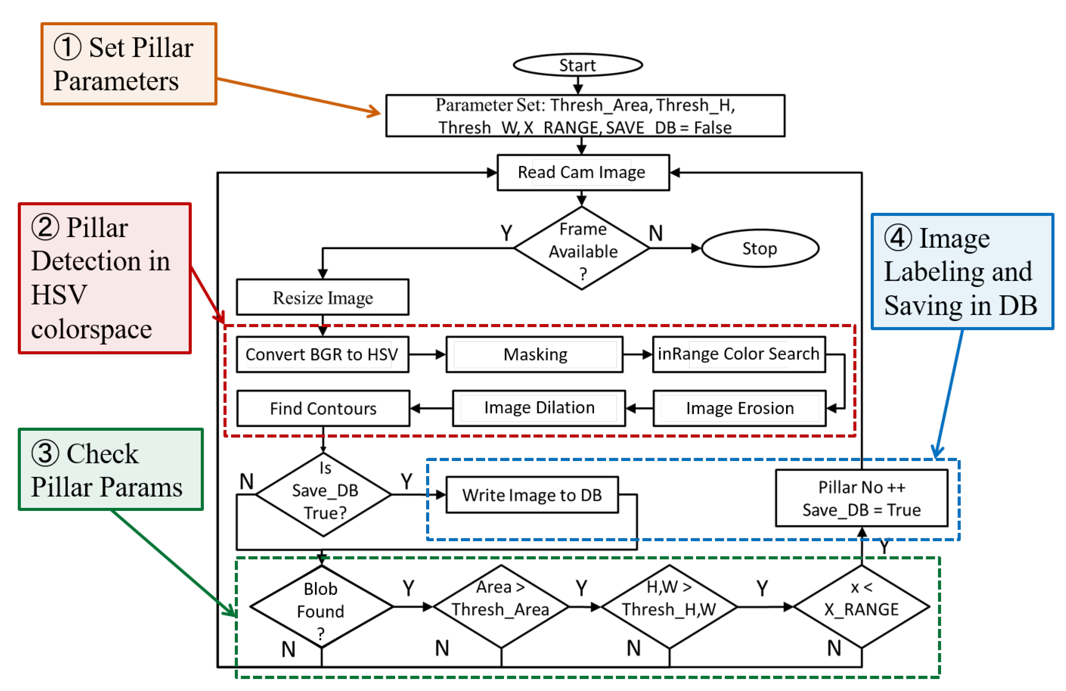
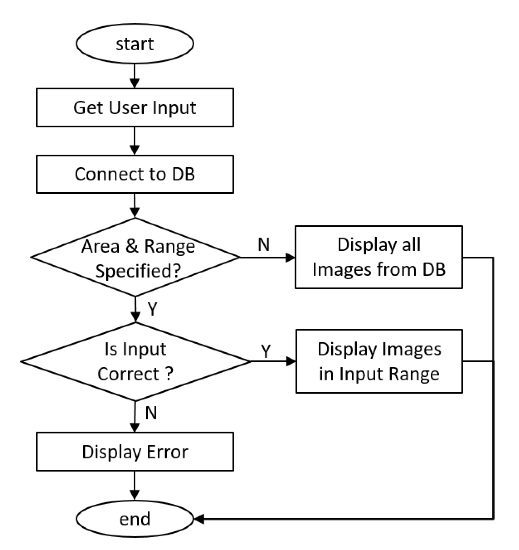
Feature detection is important for labeling image data. In the proposed method, pillars setup in the vineyards to support the grape plants are detected as features using image processing. The algorithm to detect pillars is given in the flowchart of Figure 2. The algorithm is divided into four parts:

• Setting Pillar Parameters: We first set the static parameters used for pillar detection. These includes the approximate width ($\mathrm{Thresh}\_\mathrm{W}$) and height ($\mathrm{Thresh}\_\mathrm{H}$) of the pillars, the approximate threshold area of detection ($\mathrm{Thresh}\_\mathrm{Area}$), and the range in the horizontal axis of image within which pillars should be detected ($\mathrm{X}\_\mathrm{RANGE}$). At the start of the algorithm, a flag ($\mathrm{SAVE}\_\mathrm{DB}$) which controls the labeling and saving of images in the database is set to $\mathrm{False}$.
• Pillar Detection in HSV Colorspace: The camera setup on the robot reads an RGB color image when the robot starts to move. The camera reads the image in full HD (1920 × 1080) pixel resolution. This image is resized to $768\times 432$ pixels for faster image processing. Next, pillars are detected in HSV colorspace and the various steps are explained below:
  • BGR to HSV Conversion: The resized RGB image (${\mathit{I}}_{rgb}$) is converted to HSV colorspace. Unlike RGB (Red, Green, and Blue channel image), HSV (Hue, Saturation, and Value) separates the color information (chroma) from the image intensity (luma). This separation enables robust color detection. The RGB to HSV color conversion is done using the following equations [40]:

    $$\begin{array}{cc}\hfill V& \leftarrow \mathsf{max}(R,G,B)\hfill \\ \hfill S& \leftarrow \left\{\begin{array}{cc}{\displaystyle \frac{V-\mathsf{min}(R,G,B)}{V}},\hfill & \mathrm{if}V\ne 0\hfill \\ 0,\hfill & \mathrm{otherwise}\hfill \end{array}\right.\hfill \\ \hfill H& \leftarrow \left\{\begin{array}{cc}{\displaystyle \frac{60(G-B)}{V-\mathsf{min}(R,G,B)}},\hfill & \mathrm{if}V=R\hfill \\ {\displaystyle \frac{60(B-R)}{V-\mathsf{min}(R,G,B)}}+120,\hfill & \mathrm{if}V=G\hfill \\ {\displaystyle \frac{60(R-G)}{V-\mathsf{min}(R,G,B)}}+240,\hfill & \mathrm{if}V=B\hfill \end{array}\right.\hfill \end{array}$$

    (1)
    If $H<0$, then $H\leftarrow H+360$. The range of values are: $0\le V\le 1,0\le S\le 1,0\le H\le 360$.
  • Masking: The image contains information about the grapes (mainly in middle), leaves, weed (at the bottom), and soil (at bottom). We mask the top and bottom areas to focus only on pillar detection. This masking is achieved by setting pixels in certain range of the HSV image (${\mathit{I}}_{hsv}$) to zero value as follows:

    $$\begin{array}{c}\hfill {\mathit{I}}_{hsv}[M_{Hs}:M_{He},M_{Ws}:M_{We},C_H]\leftarrow 0\\ \hfill {\mathit{I}}_{hsv}[M_{Hs}:M_{He},M_{Ws}:M_{We},C_S]\leftarrow 0\\ \hfill {\mathit{I}}_{hsv}[M_{Hs}:M_{He},M_{Ws}:M_{We},C_V]\leftarrow 0\end{array}$$

    (2)
    In Equation (2), $M_{Hs}$ and $M_{He}$ represent the masking range’s start and end points in perpendicular direction (along y-axis), respectively. Similarly, $M_{Ws}$ and $M_{We}$ represents the masking range’s start and end points in horizontal direction (along x-axis), respectively. C represents the specific channel of the image ${\mathit{I}}_{hsv}$. These values are set according to the height of the crop, the position at which the camera is fixed on the robot, and the height of the robot. In this work, full masking is applied in the horizontal direction (along x-axis). This was achieved by setting $M_{Ws}$ to 0, and $M_{We}$ to the width of the image i.e., 768. Masking in vertical direction (along y-axis) was done in two levels. In the first level, masking was done by setting the values of $M_{Hs}$ and $M_{He}$ to 0 and 298, respectively. In the second level, masking was done by setting the values of $M_{Hs}$ and $M_{He}$ to 370 and 432, respectively. Masking was done in all the three channels. The result of masking with dimensions is shown in Figure 3.
  • Color Search: In the next step, we search for the pillar color within an $\mathsf{upper}\_\mathsf{range}$ and $\mathsf{lower}\_\mathsf{range}$. These values are set by taking a snapshot of all the pillars in the vineyard in different lighting conditions and finding the lower and upper ranges of HSV values. In this work, $\mathsf{upper}\_\mathsf{range}$ was set to (34, 110, 255) and $\mathsf{lower}\_\mathsf{range}$ was set to (17, 26, 50) for the H, S, and V values. The result of color search in this range is a binary image (${\mathit{I}}_b$). If the pixel values of ${\mathit{I}}_{hsv}$ is within the upper and lower ranges, the respective pixel in ${\mathit{I}}_b$ is set to white ($\mathsf{0}\mathsf{xFF}$), or zero, otherwise.

    $$\begin{array}{c}\hfill {\mathit{I}}_b\leftarrow \left\{\begin{array}{cc}\mathsf{0}\mathsf{xFF},\hfill & \mathrm{if}{\{\mathsf{lower}\_\mathsf{range}\le {\mathit{I}}_{hsv}\le \mathsf{upper}\_\mathsf{range}\}}_{ch}\forall ch\in \{H,S,V\}\hfill \\ \mathsf{0},\hfill & \mathrm{otherwise}\hfill \end{array}\right.\end{array}$$

    (3)
  • Noise Removal Using Erosion and Dilation: Noise is removed from the binary image ${\mathit{I}}_b$ by applying morphological operations [41] of erosion followed by dilation. Both the operations use a structuring element ($\mathsf{SE}$), which is used to process the image. Erosion removes pixels, whereas dilate adds pixels based on the structuring element [40]. We first apply erosion operation, which removes the small and independent noise pixels. This operation affects the entire image. Therefore, dilate operation is applied afterwards.

    $$\begin{array}{cc}\hfill {\mathit{I}}_{be}& \leftarrow \underset{(x^{\prime },y^{\prime })\in \mathtt{SE}}{min}{\mathit{I}}_b(x+x^{\prime },y+y^{\prime })\hfill \\ \hfill {\mathit{I}}_b& \leftarrow \underset{(x^{\prime },y^{\prime })\in \mathtt{SE}}{max}{\mathit{I}}_{be}(x+x^{\prime },y+y^{\prime })\hfill \end{array}$$

    (4)
  • Detecting Contours: The next step involves retrieving contours from the noise removed binary image ${\mathit{I}}_b$ using the algorithm [42]. Each contour is stored as a vector of points. In this research, only the extreme outer contours are retrieved. Hence, each contour $c_i$ is a vector of five parameters: $x_i,y_i,w_i,h_i$, and $a_i$. Here, $x_i$ and $y_i$ are the coordinates of the top-left coordinates of the contour ($c_i$), respectively. Moreover, $a_i$ is the contour area, with $w_i$ and $h_i$ the width and height of the contour ($c_i$), respectively.
• Checking Detected Pillar’s Dimensions: If n contours are detected, then the dimensions of each contour are checked. Using the contour parameters $x_i,y_i,w_i,h_i$, and $a_i$, the condition for pillar detection is done using Algorithm 1.
• Image Labeling and Saving in Database: The $\mathrm{SAVE}\_\mathrm{DB}$ controls the semantic indexing of image data in the robot’s database. For each frame, the $\mathrm{SAVE}\_\mathrm{DB}$ is set to the output of Algorithm 1. When the $\mathrm{SAVE}\_\mathrm{DB}$ flag is $\mathrm{True}$, the pillar number is incremented, and successive images are logged based on the new pillar index.

Algorithm 1: Contour check for pillar.

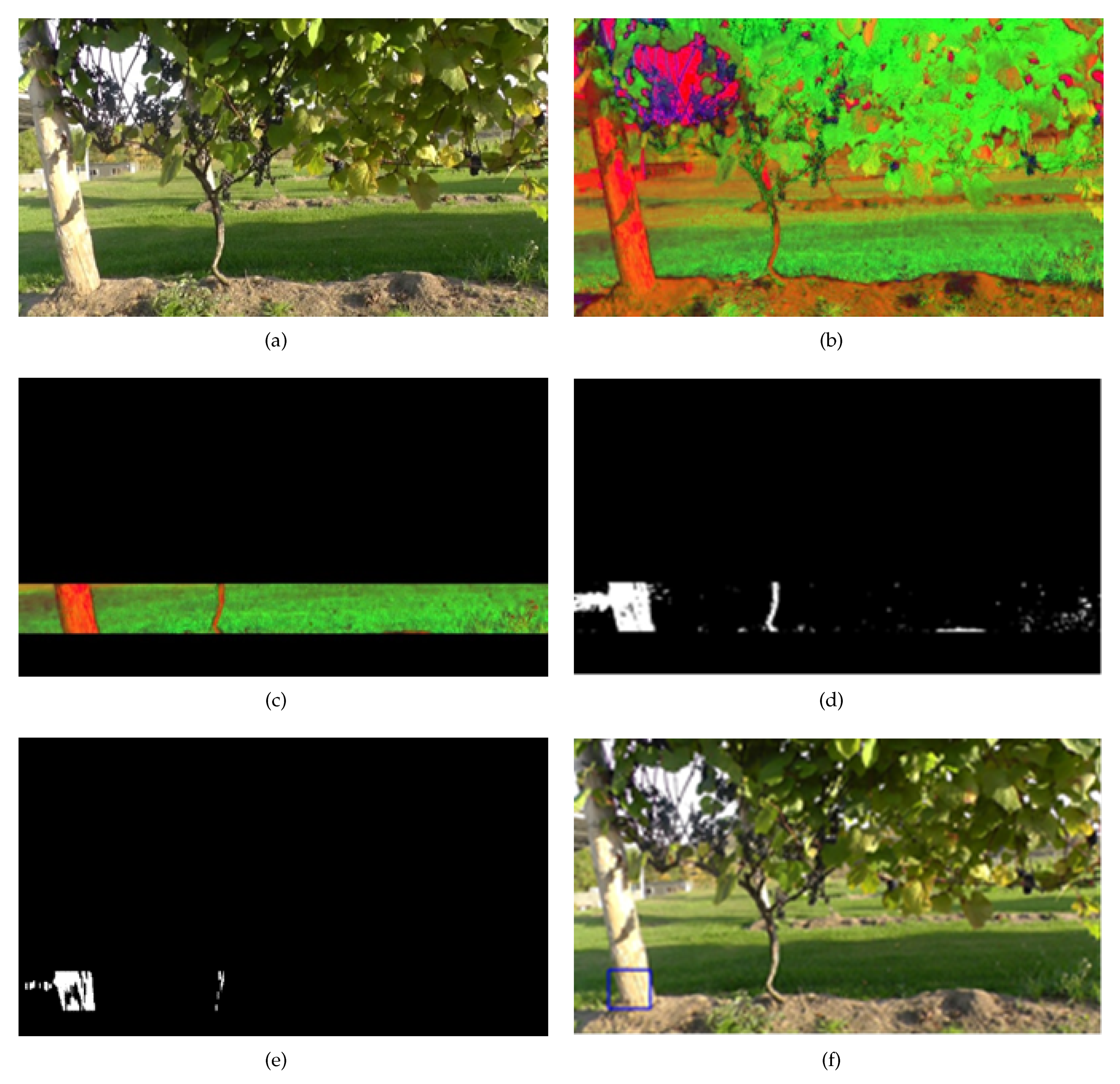
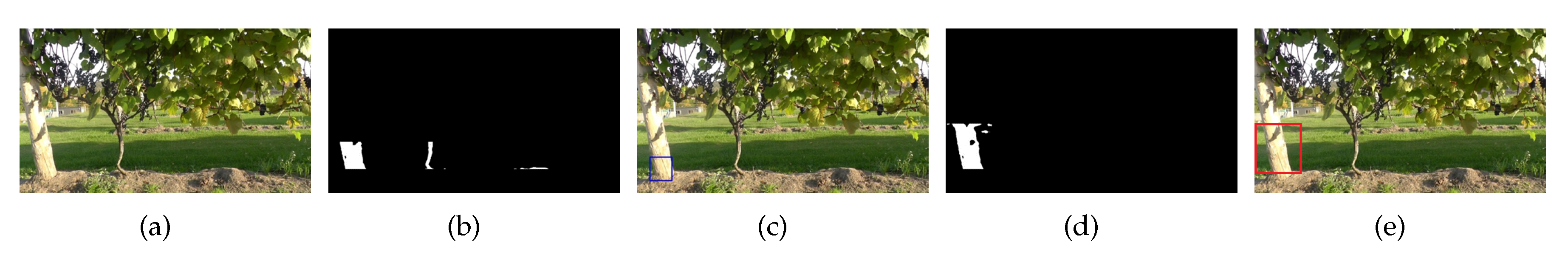
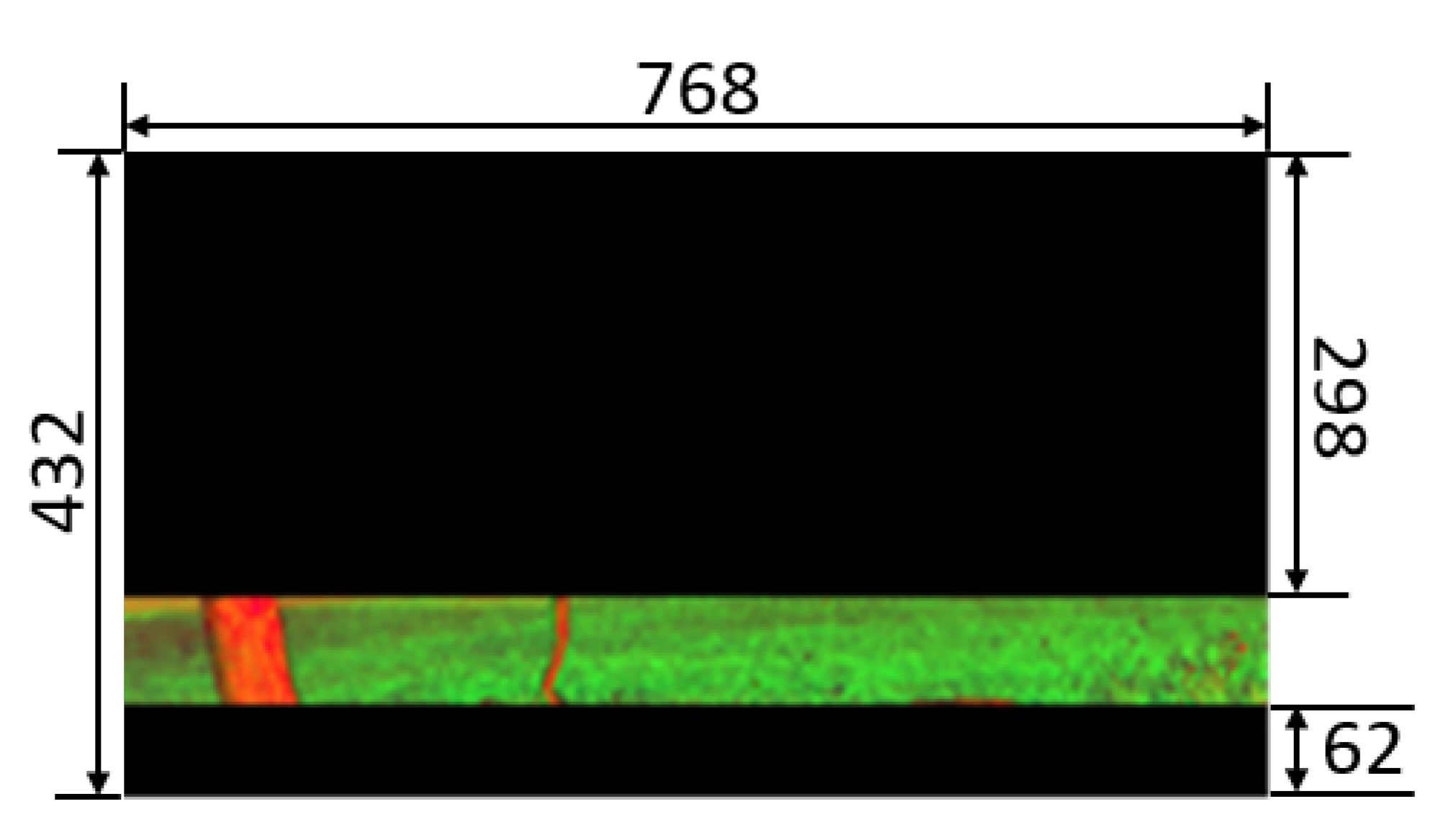
Figure 4 shows the results of the pillar detection. Figure 4a is the resized $768\times 432$ input image in RGB colorspace. Figure 4b shows the image ${\mathit{I}}_{hsv}$ which has been converted to HSV colorspace. Masking is applied to avoid detection of pillars and soil in the background. Figure 4c shows the result of masking. Color of the pillar is searched in this image between the $\mathsf{upper}\_\mathsf{range}$ of (34, 110, 255) and $\mathsf{lower}\_\mathsf{range}$ of (17, 26, 50) and the resultant binary image ${\mathit{I}}_b$ is shown in Figure 4d. In this image, the white pixels are those whose values fall within the color search range. It can be seen that the pillar and stem of the grape plant are predominantly emphasized by this operation. At the same time, noise can also be seen in the image as small and independent white blobs. By applying morphological operations of erosion and dilation, noise is removed and the result is shown in Figure 4e. Finally, contours are retrieved from the noise removed image, and parameters of contour’s width, height, area, etc. are checked for detecting the pillar. The result of the detected pillar is shown in Figure 4f, in which the detected pillar is marked by a blue rectangle.

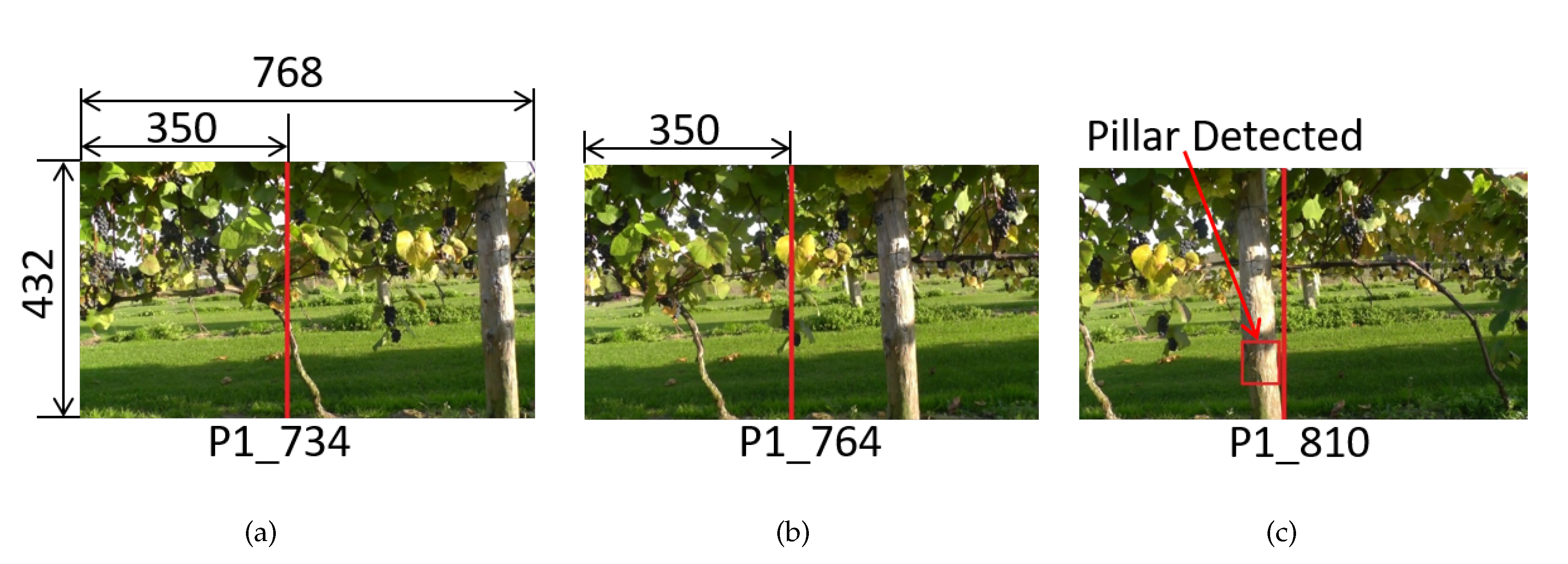
Effect of X-Range Parameter

Section 3 described many parameters which were used in the pillar detection algorithm. Among these, one of the parameters $\mathrm{X}\_\mathrm{RANGE}$ is briefly explained here. This parameter sets the range in the horizontal axis of the image within which a pillar should be detected. In the proposed work, the value of $\mathrm{X}\_\mathrm{RANGE}$ is set to 350. Thus, pillars are detected only within $x<350$. The same pillar detected at different angles has varying height, width, and area. Therefore, different thresholds need to set for different angles. Hence, for accurate estimation, the pillar is said to be detected only when the line joining the camera and the pillar are perpendicular to the direction of robots motion. The effect of this parameter on pillar detection is shown in Figure 5. In Figure 5a, a red vertical line is shown at $x=350$. A pillar appears on the right side of the line. Although visible, it is not detected at this stage. As the robot moves, the pillar gets close to the red vertical line, as shown in Figure 5b. Finally, when the pillar’s top-left x-coordinate is within $\mathrm{X}\_\mathrm{RANGE}$ and the other conditions of height, width, and area are satisfied, the pillar is detected, as shown in Figure 5c.

Section 3 describes masking to produce a horizontal band of HSV pixels. The results of this masking are shown in Figure 3 and Figure 4c. This was performed to avoid detection of pillars and soil in the background. Moreover, masking was not applied for areas where $x>\mathrm{X}\_\mathrm{RANGE}$. This is because the algorithm has an alert feature which tracks soon to appear pillars for safety.

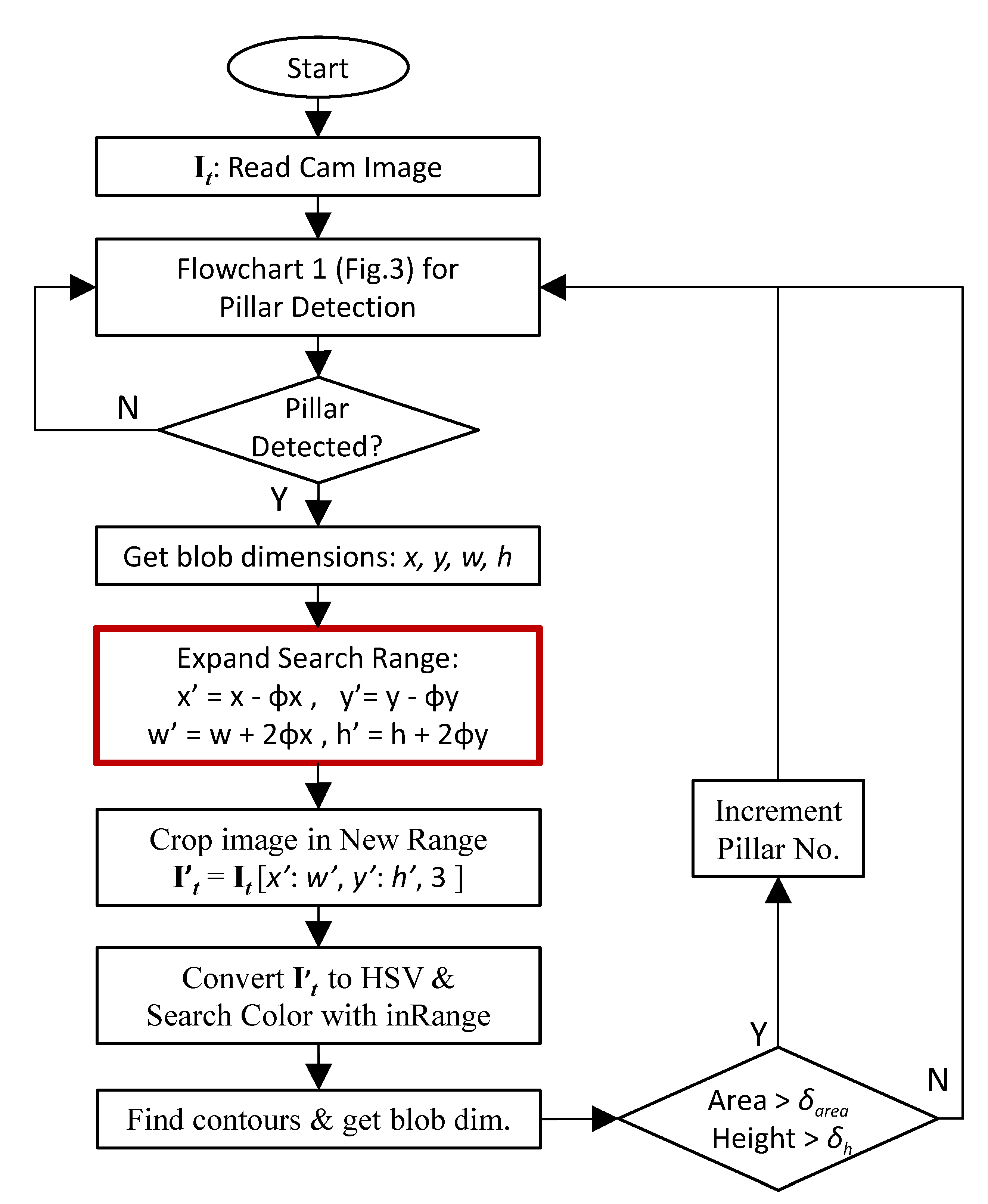
4. Improving the Robustness of Pillar Detection Algorithm

In real-world scenarios, it is possible that an object (e.g., box) whose color resembles the color of pillars is kept in the vineyard. This may lead to false data logging. To avoid this, it is important to improve the robustness of the algorithm. To do this, once a pillar has been detected using the algorithm described in Section 3, the pillar is searched again within a larger search-space.

The algorithm is shown in Figure 6. The algorithm begins by reading image from the camera and initial pillar detection is done according to the flowchart given in Figure 2. If a pillar is detected, the flowchart in Figure 2 outputs the blob dimensions $x,y,w,h$, and a representing the top-left x-coordinate and y-coordinate, width, height, and area of the detected pillar, respectively. As shown in Figure 6, the search range is then expanded based on the parameters retrieved from initial detection. This expansion is done using two parameters ${\varphi }_x$ and ${\varphi }_y$, which control the expansion of the search range on x-axis and y-axis, respectively. The parameter ${\varphi }_x$ is a vector of ${\varphi }_{xl}$ and ${\varphi }_{xr}$, which represent expansion in the left and right directions along the x-axis, respectively. Similarly, the parameter ${\varphi }_y$ is a vector of ${\varphi }_{yu}$ and ${\varphi }_{yd}$, which represent expansion in the up and down directions along the y-axis, respectively.

$$\begin{array}{cc}\hfill {\varphi }_x& =\{{\varphi }_{xl},{\varphi }_{xr}\}\hfill \\ \hfill {\varphi }_y& =\{{\varphi }_{yu},{\varphi }_{yd}\}\hfill \end{array}$$

(5)

If $x,y,w,h$, and a are the dimensions of the pillar detected using the flowchart in Figure 2, the pillar is searched again in an expanded range given by parameters $x^{\prime },y^{\prime },w^{\prime }$, and $h^{\prime }$, which are given as:

$$\begin{array}{cc}\hfill x^{\prime }& \leftarrow x-{\varphi }_{xl}\hfill \\ \hfill y^{\prime }& \leftarrow y-{\varphi }_{yu}\hfill \\ \hfill w^{\prime }& \leftarrow w+{\varphi }_{xl}+{\varphi }_{xr}\hfill \\ \hfill h^{\prime }& \leftarrow h+{\varphi }_{yu}+{\varphi }_{yd}\hfill \end{array}$$

(6)

The HSV colorspace image ${\mathit{I}}_{hsv}$ is cropped with the dimensions given in Equation (6) generating an image ${\mathit{I}}_t$. Color is then searched in this cropped image within an $\mathsf{upper}\_\mathsf{range}$ and $\mathsf{lower}\_\mathsf{range}$. The values of these limits are the same as used in Section 3, and $\mathsf{upper}\_\mathsf{range}$ is (34, 110, 255) and $\mathsf{lower}\_\mathsf{range}$ is (17, 26, 50) for the H, S, and V values. This results in a binary image ${{\mathit{I}}^{\prime }}_t$. Noise is removed using erosion and dilation and contours are retrieved using the algorithm given in [42]. The dimensions of the detected contours are checked against new thresholds of height (${\delta }_h$) and area (${\delta }_{area}$). As shown in Figure 6, if the conditions are satisfied, the pillar is said to be detected, and pillar number counter is incremented.

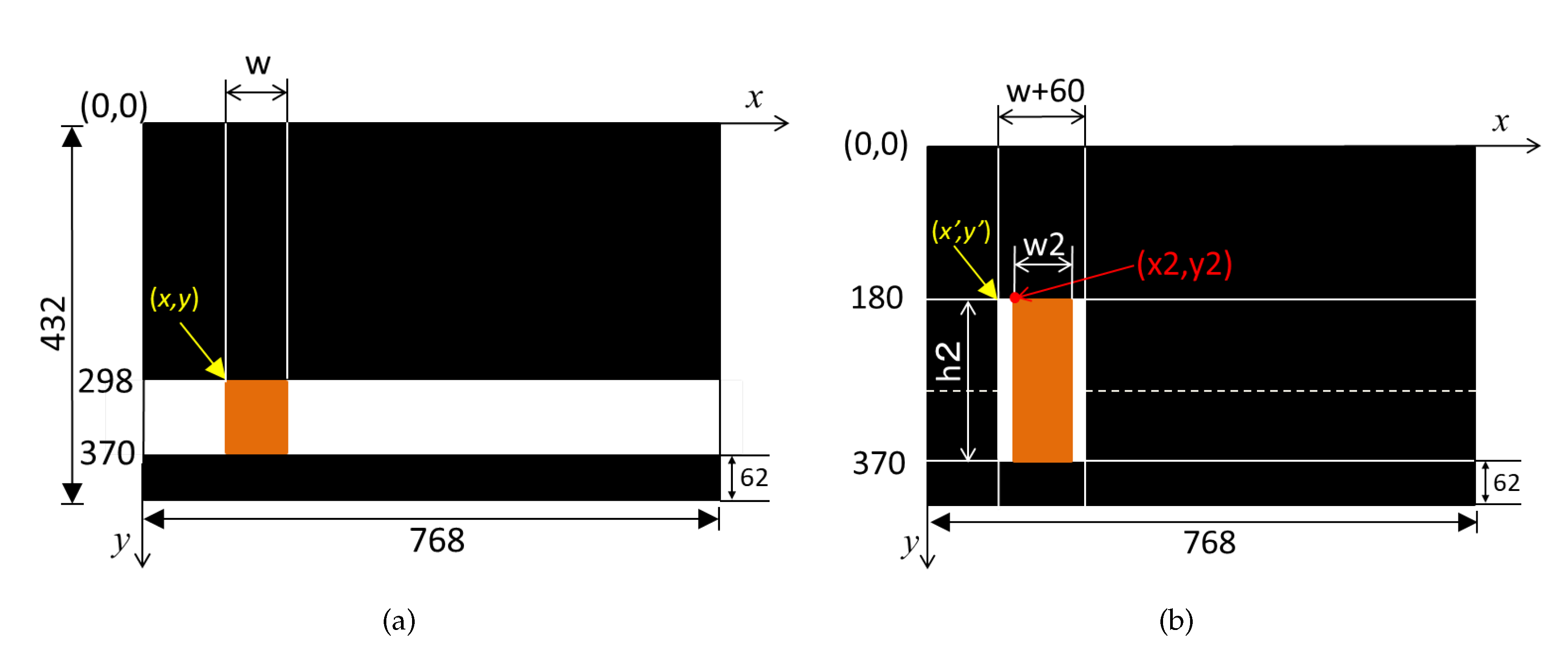
Figure 7 shows the initial range detection and expanded range detection used in this work. The initial detection range is shown in Figure 7a. It can be seen that the pillar is detected within $y=298$ and $y=370$ over the entire x-axis. Once the pillar is detected, the range is expanded, as shown in Figure 7b. In this work, the parameters given in Equation (6) are set as below:

$${\varphi }_{xl}\leftarrow 30,{\varphi }_{xr}\leftarrow 30,{\varphi }_{yu}\leftarrow 118,{\varphi }_{yd}\leftarrow 0.$$

(7)

This expands the search range for pillar detection between $y=180$ and $y=370$ along the y-axis and between $x-30$ and $x+w+60$ along the x-axis, as shown in Figure 7b. Note that ${\varphi }_{yd}$ is set to 0 to avoid noise due to soil. The initial detection in narrow range is performed for faster detection. Once a pillar has been detected, search range is expanded and pillar is detected again for robustness.

5. Semantic Data Logging and Monitoring System

This section explains the format of data logging used in the proposed work, and the monitoring system.

5.1. Semantic Data Logging in Vineyard

Data are semantically logged in the robot’s database in the format shown in Figure 8. This is the format in which image captured from the camera is named and saved in the robot’s database. Different sections of the image filename are separated by hyphen. The first section of the filename is the field name, which could be set arbitrarily by the field owner. The second section of the filename is the type of the grape. The third section is the lane number. The fourth section is the pillar number, which is followed by the frame number. In addition, the database also consists of a direction flag, which indicates the direction of motion of robot in forward or reverse direction. Images can be store in JPEG, PNG, or RAW format. An example of semantic data is shown below.

‘Kitami – Kiyomai – L5 – P3 – 108.jpg’

It is evident from the filename that the image containing grape information belongs to a field in ‘Kitami’, the type of grape is ‘Kiyomai’. ‘Kiyomai’ is a grape type cultivated in Hokkaido region of Japan. It is a crossbreed of Crimson glory vine and Kiyomi grape. Kiyomi grape is a clone version of Seibel 13053 (see [16]). The image belongs to Lane 5, and it is the 108th image from the third pillar. The precise date and time of the image can be accessed indirectly by referring the properties of the image or it can be directly stored in the database. Separating different sections of the image filename also simplifies programming while displaying the images to the farmers through the monitoring system.

5.2. Monitoring System

Figure 9 shows the simplified flowchart of the monitoring software. It starts with a user interface through which the farmer interacts. It first connects to the local or remote database. The farmer specifies the field name, lane number, and pillars between which the field is to be monitored. If the lane number is not specified, all the lanes are shown. If a lane number is specified but the pillar number is not specified, all the images in that lane are shown to the farmer. The farmer can skip through the vineyard images on a pillar by pillar basis by pressing the ‘Esc’ key. In case of wrong input, an error is displayed.

6. Experiments in Real Field and Results

Figure 10 shows the experiment setup. We performed experiments in a vineyard located in Hokkaido prefecture of Japan, as shown in Figure 10a. The pillars in this vineyard are separated by about 2.9 m. The diameter of the pillar is between approximately 13 and 16 cm. The grape plants are planted about 40 cm above the ground. The maximum height of the grape plants is 1.6 m.

The Summit XL robot (Figure 10b) [43] was used in the experiment, which is a four-wheel drive robot. It was equipped with a lightweight (≈370 g) Hokuyo UTM-30LX Lidar sensor [44]. This sensor has a range of 30 m and a scanning angle of 270 degrees. The angular resolution is 0.25° and the scan time is 25 ms/scan. The sensor has an accuracy of ±30 mm within 0.1–10 m, and ±50 mm between 10 and 30 m. The Lidar was used for robot localization and mapping (SLAM) using the algorithm proposed in [37,38].

The robot was also equipped with a Logicool C920 camera facing the grapes. The camera was used for logging image data. The robot was programmed using a control computer with Intel Core-i5 processor, 8 GB RAM, and Ubuntu Linux operating system. MySQL software was used for database. Robot programming was done using Robot Operating System (ROS) [45].

6.1. Results of Pillar Detection for Semantic Labeling

Figure 11 shows the results of pillar detection in a particular lane of the vineyard for semantic labeling. We briefly explain the results with Figure 11, which shows the first pillar detection results. The description of the other pillar’s detection is similar and therefore omitted for brevity.

Figure 11 shows the first pillar detection of a lane in the vineyard. Figure 11a shows the RGB color image captured from the camera and resized. This image is converted to HSV colorspace in which the pillar’s color is detected resulting in binary image. Contours are then detected in the binary image after noise removal and the result is shown in Figure 11b. After checking various thresholds of height, width, and area, the pillar is detected, as shown by a blue rectangle in Figure 11c. This is the result of initial detection of the algorithm explained in Section 3.

Using the dimensions of the initial detection, the search range in the HSV colorspace is expanded, as explained in Section 4, and the pillar’s color is checked once again. The binary image from this detection is shown in Figure 11d. Contours are retrieved again and finally the pillar is detected, as shown in Figure 11e.

6.2. Processing Time for Pillar Detection

Table 1. Processing time of each frame for pillar detection.

Function	Time (ms)
Image resize	6.71
BGR to HSV Conversion	2.41
Masking	0.88
Pillar’s color search	0.88
Erode and Dilate	4.08
Contours Detection	0.40
Image Labeling and DB Save	23.19
Total	38.55

summarizes the processing time of each frame for pillar detection. The total time required is around 40 ms per frame. Apart from this, around 15 ms is required for pillar detection in expanded search space. However, this extra time is only required once when a pillar is detected in a smaller search space. Since we resize the image, a faster processing time has been achieved. It should be noted that, although processing is done using the resized image, an actual full sized HQ image can be saved in the database after each detection.

6.3. Vineyard Monitoring System

The monitoring system was programmed in Python 3.6 using Matplotlib, NumPy, and OpenCV libraries. MySQL database was used. The farmer accessed the system on a Windows tablet PC. The database was downloaded on the local machine. At the current stage, the monitoring system uses command line interface. A snapshot of the software is shown in Figure 12. The farmer can pin-pointedly monitor the vineyard using the following command:

C : \ > python monitor.py field=<field-name> lane=<Lane-No.> pillar=<Pillar-No.>

The user specifies the field name, range of lane numbers, and range of pillar numbers which are to be monitored. By default, the most recent data are shown. A concrete example is given below:

C : \ > python monitor.py field = Kiyomai lane = L5 pillar = P1 − P4

As shown in Figure 12, the above command specifies the field name (Kiyomai), Lane 5, and pillar range $\mathrm{P}1$ to $\mathrm{P}4$. This shows only the images in the range specified by the user. As an example, the first image is shown in Figure 12. The software displays the image with certain information, e.g., $\mathrm{P}1-1$, which indicates that this is the first image among all the images starting from pillar $\mathrm{P}1$. The lane number is 5 and the field is Kiyomai. The detected pillars are also shown. The software successively displays the next image with information: $\mathrm{P}1-2,\mathrm{P}1-3,\cdots ,\mathrm{P}1-\mathrm{n}$, where n is the last image from pillar $\mathrm{P}1$ until the detection of the next pillar $\mathrm{P}2$. From the next pillar $\mathrm{P}2$, the images are shown with information: $\mathrm{P}2-1,\mathrm{P}2-2,\cdots ,\mathrm{P}2-\mathrm{m}$, where m is the last image from pillar $\mathrm{P}2$. This sequence is continued until pillar $\mathrm{P}4$.

This is illustrated in Figure 13, which shows selected outputs of the monitoring system for Lane 5 and Pillars 1–4. Figure 13a shows the first image of output. The successive image from Pillar 1 are also displayed, as shown in Figure 13b (241st image from Pillar 1) and Figure 13c (507th image from Pillar 1). Finally, Figure 13d shows the last image. It can be seen that the next pillar appears in the scene. Figure 13e shows the first image from Pillar 2, and subsequently Figure 13h is the last image from Pillar 2. Similarly, Figure 13i shows the first image from Pillar 3, and subsequently Figure 13l is the last image from Pillar 3.

It should be noticed that the total number of images between different pictures is different. This is because, even if the robot navigates at a constant speed, the distances between different pillars are not the same. Readers are strongly advised to see the attached video for better comprehension of the monitoring software.

A minimal setup of the proposed monitoring system per se can be realized using an inexpensive processing board (e.g., Raspberry-Pi 4 board), a web-camera, and a storage device. Using this equipment, a minimal setup is possible for under 100 USD (as of May 2020) while noting that the cost of computing decreases day-by-day [46]. This estimate excludes the cost of the autonomous robots on which the setup will be installed. However, the setup can be used in conjunction with already existing robots used for tasks such as weed removal.

Robust feature (pillar) detection is a critical component of the proposed monitoring system. Since the proposed work uses only cameras for feature detection, illumination changes are taken care using various thresholds. However, under very low illumination (e.g., during evening or very cloudy days), it is difficult to set the correct thresholds and features might not be detected robustly. Since an on-board large database access is not always feasible, the proposed system requires access to a server through a network. In remote areas, network unavailability can be another possible technical limitation over a long time.

7. Conclusions

Viticulture involves many labor intensive tasks. Among these tasks, vineyard monitoring is a task which is often done frequently to check the growth of grapes and damage. To sustain viticulture in countries such as Japan which have increasing old-age population, it becomes important to support viticulture activities using robots and AI. To this end, this research proposed a low-cost monitoring system for vineyards. The proposed system uses only low-cost cameras to semantically label the image data. This semantic labeling enables the farmers to pin-point the location which needs to be monitored. The proposed system detects pillars setup in the vineyard as features to label the image data. An algorithm to improve the robustness of pillar detection was proposed by detecting the pillar in a larger search space. The entire system is comprised of only a camera and a computer. The proposed system does not require a high-end computer and embedded boards such as Raspberry-Pi can also be used for real-time processing. Due to its compactness, the system is portable and can be installed on already existing autonomous robots used in vineyards. We tested the proposed monitoring system in actual vineyards with real robots. The results show that, unlike images captured from UAVs or drones, the proposed system can provide high quality images of grapes from short distance, which enables better monitoring of the vineyard. Moreover, pin-pointed semantic monitoring enables farmers to check only specific areas of the vineyard. The proposed system can provide monitoring on both local and online devices. In its present state, the proposed monitoring system uses a command line interface for monitoring. In the future, we plan to improve the system by providing a graphical user interface for farmers. Moreover, the present study was limited to a single vineyard. In the future, we plan to implement the proposed monitoring system in different vineyards and estimate the farmer’s satisfaction level.

References

1. Ye, F.; Qi, W. Design of wireless sensor node for drought monitoring in vineyards. In Proceedings of the International Conference on Advanced Infocomm Technology 2011 (ICAIT 2011), Wuhan, China, 11–14 July 2011; Volume 2011, pp. 1–4. [Google Scholar] [CrossRef]
2. Sánchez, N.; Martínez-Fernández, J.; Aparicio, J.; Herrero-Jiménez, C.M. Field radiometry for vineyard status monitoring under Mediterranean conditions. In Proceedings of the 2014 IEEE Geoscience and Remote Sensing Symposium, Quebec City, QC, Canada, 13–18 July 2014; pp. 2094–2097. [Google Scholar]
3. Wigneron, J.; Dayan, S.; Kruszewski, A.; Aluome, C.; AI-Yaari, M.G.A.; Fan, L.; Guven, S.; Chipeaux, C.; Moisy, C.; Guyon, D.; et al. The Aqui Network: Soil Moisture Sites in the “Les Landes” Forest and Graves Vineyards (Bordeaux Aquitaine Region, France). In Proceedings of the IGARSS 2018—2018 IEEE International Geoscience and Remote Sensing Symposium, Valencia, Spain, 22–27 July 2018; pp. 3739–3742. [Google Scholar]
4. Gay-Fernández, J.A.; Cuiñas, I. Deployment of a wireless sensor network in a vineyard. In Proceedings of the International Conference on Wireless Information Networks and Systems, Seville, Spain, 18–21 July 2011; pp. 35–40. [Google Scholar]
5. Galmes, S. Lifetime Issues in Wireless Sensor Networks for Vineyard Monitoring. In Proceedings of the 2006 IEEE International Conference on Mobile Ad Hoc and Sensor Systems, Vancouver, BC, Canada, 9–12 October 2006; pp. 542–545. [Google Scholar]
6. Medela, A.; Cendón, B.; González, L.; Crespo, R.; Nevares, I. IoT multiplatform networking to monitor and control wineries and vineyards. In Proceedings of the 2013 Future Network Mobile Summit, Lisboa, Portugal, 3–5 July 2013; pp. 1–10. [Google Scholar]
7. Mouakher, A.; Belkaroui, R.; Bertaux, A.; Labbani, O.; Hugol-Gential, C.; Nicolle, C. An Ontology-Based Monitoring System in Vineyards of the Burgundy Region. In Proceedings of the 2019 IEEE 28th International Conference on Enabling Technologies: Infrastructure for Collaborative Enterprises (WETICE), Napoli, Italy, 12–14 June 2019; pp. 307–312. [Google Scholar]
8. Ahumada-García, R.; Poblete-Echeverría, C.; Besoain, F.; Reyes-Suarez, J. Inference of foliar temperature profile of a vineyard using integrated sensors into a motorized vehicle. In Proceedings of the 2016 IEEE International Conference on Automatica (ICA-ACCA), Curico, Chile, 19–21 October 2016; pp. 1–6. [Google Scholar]
9. Pérez-Expósito, J.P.; Fernández-Caramés, T.M.; Fraga-Lamas, P.; Castedo, L. An IoT Monitoring System for Precision Viticulture. In Proceedings of the 2017 IEEE International Conference on Internet of Things (iThings) and IEEE Green Computing and Communications (GreenCom) and IEEE Cyber, Physical and Social Computing (CPSCom) and IEEE Smart Data (SmartData), Exeter, UK, 21–23 June 2017; pp. 662–669. [Google Scholar]
10. Stevenson, T. Sotheby’s Wine Encyclopedia; DK Publishers: London, UK, 2011; ISBN 0756686849. [Google Scholar]
11. Unwin, T. Wine and the Vine: An Historical Geography of Viticulture and the Wine Trade; Routledge Publishers: Abingdon, UK, 1991; ISBN 0415031206. [Google Scholar]
12. Peronospora. Wikipedia 2020. Available online: https://en.wikipedia.org/wiki/Peronospora (accessed on 31 March 2020).
13. Panagos, P.; Ballabio, C.; Lugato, E.; Jones, A.; Borrelli, P.; Scarpa, S.; Orgiazzi, A.; Montanarella, L. Potential Sources of Anthropogenic Copper Inputs to European Agricultural Soils. Sustainability 2018, 10, 2380. [Google Scholar] [CrossRef] [Green Version]
14. Gale, G. Saving the vine from phylloxera: A never-ending battle. In Wine: A Scientific Exploration; CRC Press: Boca Raton, FL, USA, 2003; pp. 70–91. [Google Scholar]
15. Japan’s Ministry of Agriculture, Forestry and Fisheries (MAFF). Grapes in Japan 2015. Available online: https://www.maff.go.jp/e/data/publish/attach/pdf/index-115.pdf (accessed on 23 March 2020).
16. Association of Japan’s Wine Lovers. List of Grape Varities in Japan. 2020. Available online: http://www.jp-wine.com/jp/kind.html (accessed on 15 April 2020).
17. Wikipedia. Grapes in Japan (Japanese). 2020. Available online: https://ja.wikipedia.org/wiki/%E3%83%96%E3%83%89%E3%82%A6 (accessed on 16 May 2020).
18. e-Stat. Statistics of Japan (Japanese). 2020. Available online: https://www.e-stat.go.jp/ (accessed on 16 May 2020).
19. Ly, O.; Gimbert, H.; Passault, G.; Baron, G. A Fully Autonomous Robot for Putting Posts for Trellising Vineyard with Centimetric Accuracy. In Proceedings of the 2015 IEEE International Conference on Autonomous Robot Systems and Competitions, Vila Real, Portugal, 8–10 April 2015; pp. 44–49. [Google Scholar] [CrossRef]
20. Igawa, H.; Tanaka, T.; Kaneko, S.; Tada, T.; Suzuki, S. Visual and tactual recognition of trunk of grape for weeding robot in vineyards. In Proceedings of the 2009 35th Annual Conference of IEEE Industrial Electronics, Porto, Portugal, 3–5 November 2009; pp. 4274–4279. [Google Scholar] [CrossRef]
21. Thayer, T.C.; Vougioukas, S.; Goldberg, K.; Carpin, S. Multi-Robot Routing Algorithms for Robots Operating in Vineyards. In Proceedings of the 2018 IEEE 14th International Conference on Automation Science and Engineering (CASE), Munich, Germany, 20–24 August 2018; pp. 14–21. [Google Scholar] [CrossRef]
22. Gao, M.; Lu, T. Image Processing and Analysis for Autonomous Grapevine Pruning. In Proceedings of the 2006 International Conference on Mechatronics and Automation, Luoyang, China, 25–28 June 2006; pp. 922–927. [Google Scholar] [CrossRef] [Green Version]
23. Thayer, T.C.; Vougioukas, S.; Goldberg, K.; Carpin, S. Routing Algorithms for Robot Assisted Precision Irrigation. In Proceedings of the 2018 IEEE International Conference on Robotics and Automation (ICRA), Brisbane, Australia, 21–25 May 2018; pp. 2221–2228. [Google Scholar] [CrossRef]
24. Riggio, G.; Fantuzzi, C.; Secchi, C. A Low-Cost Navigation Strategy for Yield Estimation in Vineyards. In Proceedings of the 2018 IEEE International Conference on Robotics and Automation (ICRA), Brisbane, Australia, 21–25 May 2018; pp. 2200–2205. [Google Scholar] [CrossRef]
25. Nuske, S.; Achar, S.; Bates, T.; Narasimhan, S.; Singh, S. Yield estimation in vineyards by visual grape detection. In Proceedings of the 2011 IEEE/RSJ International Conference on Intelligent Robots and Systems, San Francisco, CA, USA, 25–30 September 2011; pp. 2352–2358. [Google Scholar] [CrossRef] [Green Version]
26. de Sousa Contente, O.M.; Lau, J.N.P.N.; Morgado, J.F.M.; dos Santos, R.M.P.M. Vineyard Skeletonization for Autonomous Robot Navigation. In Proceedings of the 2015 IEEE International Conference on Autonomous Robot Systems and Competitions, Vila Real, Portugal, 8–10 April 2015; pp. 50–55. [Google Scholar] [CrossRef]
27. Reis, M.; Morais, R.; Peres, E.; Pereira, C.; Contente, O.; Soares, S.; Valente, A.; Baptista, J.; Ferreira, P.; Bulas Cruz, J. Automatic detection of bunches of grapes in natural environment from color images. J. Appl. Log. 2012, 10, 285–290. [Google Scholar] [CrossRef] [Green Version]
28. dos Santos, F.B.N.; Sobreira, H.M.P.; Campos, D.F.B.; dos Santos, R.M.P.M.; Moreira, A.P.G.M.; Contente, O.M.S. Towards a Reliable Monitoring Robot for Mountain Vineyards. In Proceedings of the 2015 IEEE International Conference on Autonomous Robot Systems and Competitions, Vila Real, Portugal, 8–10 April 2015; pp. 37–43. [Google Scholar]
29. Ravankar, A.; Ravankar, A.A.; Hoshino, Y.; Kobayashi, Y. On Autonomous Navigation in Vineyards with Lidar Information. In Proceedings of the IEEE SICE Annual Conference 2019 (SICE 2019), IEEE, SICE, Hiroshima, Japan, 10–13 September 2019. [Google Scholar] [CrossRef]
30. Roure, F.; Bascetta, L.; Soler, M.; Matteucci, M.; Faconti, D.; Gonzalez, J.P.; Serrano, D. Lessons Learned in Vineyard Monitoring and Protection from a Ground Autonomous Vehicle. In Advances in Robotics Research: From Lab to Market: ECHORD++: Robotic Science Supporting Innovation; Grau, A., Morel, Y., Puig-Pey, A., Cecchi, F., Eds.; Springer International Publishing: Cham, Switzerland, 2020; pp. 81–105. [Google Scholar] [CrossRef]
31. Das, J.; Cross, G.; Qu, C.; Makineni, A.; Tokekar, P.; Mulgaonkar, Y.; Kumar, V. Devices, systems, and methods for automated monitoring enabling precision agriculture. In Proceedings of the 2015 IEEE International Conference on Automation Science and Engineering (CASE), Gothenburg, Sweden, 24–28 August 2015; pp. 462–469. [Google Scholar]
32. Lloret, J.; Bosch, I.; Sendra, S.; Serrano, A. A Wireless Sensor Network for Vineyard Monitoring That Uses Image Processing. Sensors 2011, 11, 6165–6196. [Google Scholar] [CrossRef] [PubMed] [Green Version]
33. Vinbot. Vinbot 2020. Available online: http://vinbot.eu/ (accessed on 31 March 2020).
34. Ravankar, A.; Ravankar, A.; Kobayashi, Y.; Emaru, T. Hitchhiking Robots: A Collaborative Approach for Efficient Multi-Robot Navigation in Indoor Environments. Sensors 2017, 17, 1878. [Google Scholar] [CrossRef] [PubMed] [Green Version]
35. Ravankar, A.; Ravankar, A.; Kobayashi, Y.; Hoshino, Y.; Peng, C.C.; Watanabe, M. Hitchhiking Based Symbiotic Multi-Robot Navigation in Sensor Networks. Robotics 2018, 7, 37. [Google Scholar] [CrossRef] [Green Version]
36. Ravankar, A.; Ravankar, A.; Kobayashi, Y.; Emaru, T. Symbiotic Navigation in Multi-Robot Systems with Remote Obstacle Knowledge Sharing. Sensors 2017, 17, 1581. [Google Scholar] [CrossRef] [PubMed] [Green Version]
37. Ravankar, A.A.; Hoshino, Y.; Ravankar, A.; Jixin, L.; Emaru, T.; Kobayashi, Y. Algorithms and a Framework for Indoor Robot Mapping in a Noisy Environment using Clustering in Spatial and Hough Domains. Int. J. Adv. Robot. Syst. 2015, 12, 27. [Google Scholar] [CrossRef] [Green Version]
38. Ravankar, A.; Ravankar, A.A.; Hoshino, Y.; Emaru, T.; Kobayashi, Y. On a Hopping-points SVD and Hough Transform Based Line Detection Algorithm for Robot Localization and Mapping. Int. J. Adv. Robot. Syst. 2016, 13, 98. [Google Scholar] [CrossRef] [Green Version]
39. Ravankar, A.A.; Ravankar, A.; Peng, C.; Kobayashi, Y.; Emaru, T. Task coordination for multiple mobile robots considering semantic and topological information. In Proceedings of the 2018 IEEE International Conference on Applied System Invention (ICASI), Chiba, Japan, 13–17 April 2018; pp. 1088–1091. [Google Scholar] [CrossRef]
40. Bradski, A. Learning OpenCV, Computer Vision with OpenCV Library; Software That Sees, 1st ed.; Bradski, G., Kaehler, A., Eds.; O’Reilly Media: Sevastopol, CA, USA, 2008. [Google Scholar]
41. Ravankar, A.; Kobayashi, Y.; Ravankar, A.; Emaru, T. A connected component labeling algorithm for sparse Lidar data segmentation. In Proceedings of the 2015 6th International Conference on Automation, Robotics and Applications (ICARA), Queenstown, New Zealand, 17–19 February 2015; pp. 437–442. [Google Scholar] [CrossRef]
42. Suzuki, S.; Abe, K. Topological structural analysis of digitized binary images by border following. Comput. Vis. Graph. Image Process. 1985, 30, 32–46. [Google Scholar] [CrossRef]
43. Robotnik Automation. Summit-XL Robot. 2020. Available online: https://www.robotnik.eu/mobile-robots/summit-xl/ (accessed on 21 May 2020).
44. UTM-30LX Technical Specifications. 2020. Available online: https://www.hokuyo-aut.jp/search/single.php?serial=169 (accessed on 2 March 2020).
45. Quigley, M.; Conley, K.; Gerkey, B.P.; Faust, J.; Foote, T.; Leibs, J.; Wheeler, R.; Ng, A.Y. ROS: An open-source Robot Operating System. In Proceedings of the ICRA Workshop on Open Source Software, Kobe, Japan, 12–17 May 2009. [Google Scholar]
46. Cost of Computing. Wikipedia 2020. Available online: https://en.wikipedia.org/wiki/FLOPS (accessed on 15 May 2020).
Figure 1. Overview of the proposed semantic monitoring system.
Agriculture 10 00182 g001
Figure 2. Simplified flowchart of pillar (feature) detection from images.
Agriculture 10 00182 g002
Figure 3. Masking of HSV image I h s v . The range is also shown.
Agriculture 10 00182 g003
Figure 4. Pillar detection in vineyard: (a) input RGB image; (b) image I h s v in HSV colorspace; (c) Masked image; (d) binary image I b after color search between upper _ range and lower _ range ; (e) image I b with noise removed after erode and dilate operations; and (f) pillar detected after finding contours and checking parameters. Detection is shown as a blue rectangle.
Agriculture 10 00182 g004
Figure 5. Pillar detection within horizontal threshold of X _ RANGE = 350 shown as red line: (a) a new pillar appears on the right side of the frame; (b) image captured as the robot moves forward, where the pillar is not detected as it is not within X _ RANGE ; and (c) pillar is recognized as it is within X _ RANGE .
Agriculture 10 00182 g005
Figure 6. Flowchart of pillar detection in expanded range after initial detection.
Agriculture 10 00182 g006
Figure 7. Search range in small range and expanded range: (a) search range for initial detection; and (b) expanded range based on coordinates retrieved from initial detection.
Agriculture 10 00182 g007
Figure 8. Format of data logging showing different sections separated by hyphen.
Agriculture 10 00182 g008
Figure 9. Simplified flowchart of monitoring software.
Agriculture 10 00182 g009
Figure 10. Experiment setup: (a) vineyard where experiments were performed; and (b) robot setup.
Agriculture 10 00182 g010
Figure 11. Robust pillar detection in vineyard (Pillar-1): (a) input RGB image; (b) binary image generated after noise removal from HSV image; (c) initial pillar detection in small search range; (d) binary image with pillar detection in enlarged search range; and (e) detected pillar.
Agriculture 10 00182 g011
Figure 12. A snapshot of monitoring software.
Agriculture 10 00182 g012
Figure 13. Output of monitoring software for command: field = Kiyomailane = L 5 pillar = P 1 P 4 : (a) initial image from Pillar 1; (b,c) intermediate images; (d) last image from Pillar 1; (e) initial image from Pillar 2; (f,g) intermediate images; (h) last image from Pillar 2; (i) initial image from Pillar 3; (j,k) intermediate images; and (l) last image from Pillar 3. Please see the video provided in the Supplementary Materials.
Agriculture 10 00182 g013