1. Introduction
The beekeeping industry in Western Australia has grown rapidly in the past decade, from 660 registered beekeepers in 2010 to over 3000 in 2019 [
1]. In addition, honey produced from Western Australia has some of the highest antimicrobial properties known for honey [
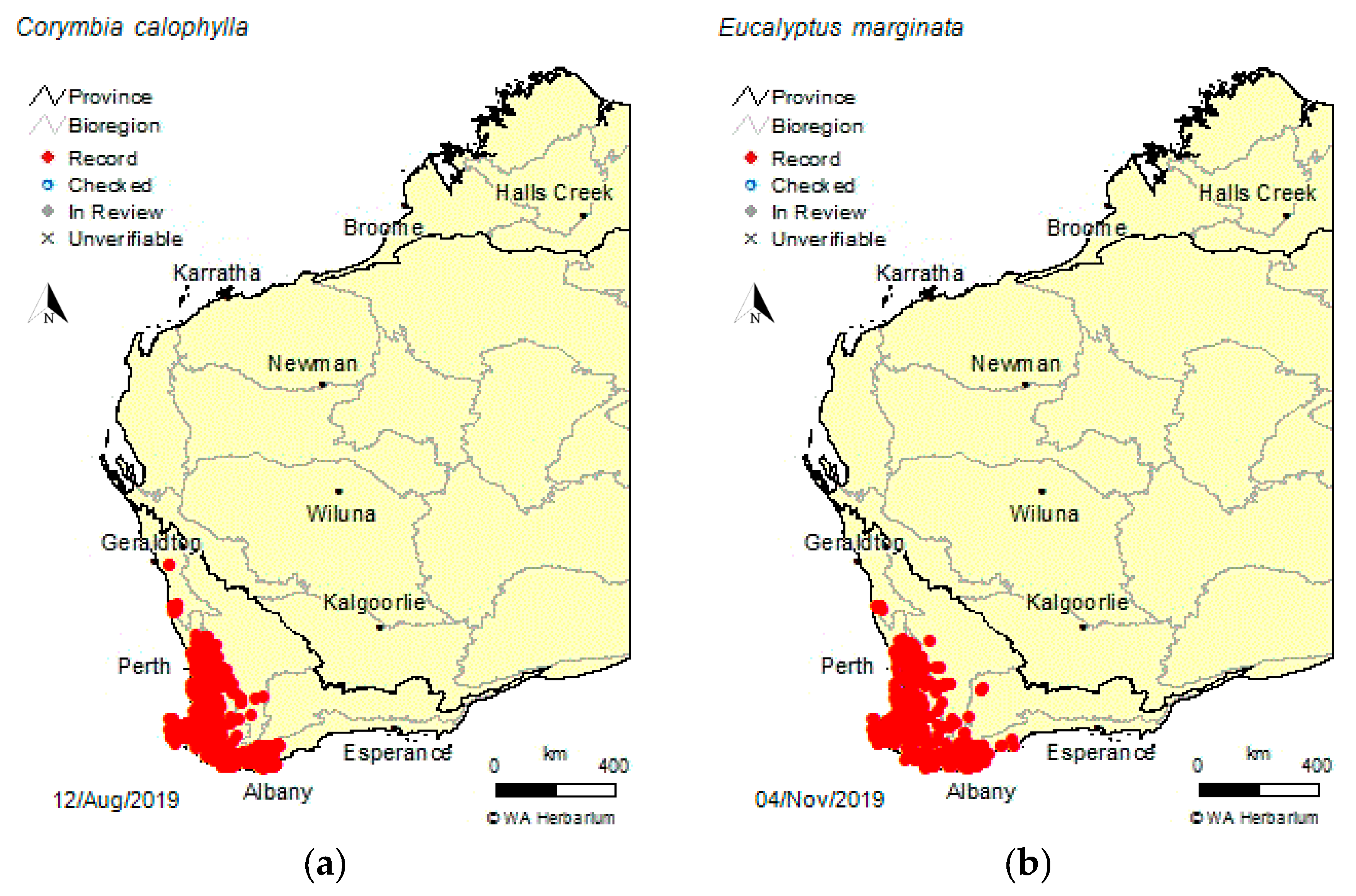
2]. As these high antimicrobial honey varieties are produced from marri (
Corymbia calophylla, Myrtaceae) and jarrah (
Eucalyptus marginata, Myrtaceae) trees that occur across a large area (see
Figure 1) of approximately 84,000 km
2 [
3], beekeepers often travel long distances to inspect apiary sites and manage their beehives. Access to a tool to predict areas of higher and lower honey production would make apiary management more efficient and improve industry safety by reducing the amount of rural driving required.
Efforts to predict flowering patterns of Myrtaceous trees in Australia from weather data have often found complex relationships between weather and phenology. For example, a phenological study of four different species of
Eucalyptus with coincident geographic ranges analysed 400 data points of flowering status and climate over 30 years [
4] with the Generalised Additive Model for Location, Scale and Shape (GAMLSS) technique to assess the impact of minimum, mean and maximum temperature for the flowering period of those species, as well as flowering intensity in the preceding months and season. This study found that there is a non-linear relationship between temperature and flowering intensity, both of which varied between the four species. Two species flowered more intensely with increasing maximum temperatures, one species flowered more intensely with increasing minimum temperature and one species flowered less intensely with increasing maximum temperature. While temperature was consistently a key factor in flowering intensity, the effect was far from consistent.
While several studies on the relationship between satellite-derived vegetation indices and honey production in south-east Australia have shown promising outcomes [
5,
6,
7], these have been qualitative in nature, with no demonstration of quantitative relationships, nor predictive model development.
Hawkins and Thomson [
8] developed a qualitative, relativistic model for landscape/regional scale nectar availability in subtropical Eastern Australia, covering an area of 314,400 Ha. This study identified some key factors that were related to nectar availability, notably the Gross Primary Productivity for the previous 12 months and the average annual solar radiation and rainfall for the previous 6 months. The study was broad, covering more than 50 different plant species from many different genera.
In this paper, we use machine learning regression methods to assess the capability of both weather data and satellite-derived vegetation and moisture related data to develop a honey harvest prediction model for marri honey. This includes an assessment of the spatial density of weather station data from the Australian Government’s Bureau of Meteorology (BOM). The primary aim is to identify the key factors that influence marri honey production and identify potential limitations in the data sources for these key factors.
2. Materials and Methods
2.1. Honey Harvest Data
Honey harvest data used for this study were from the same dataset used by Campbell, Fearns [
9]. The dataset is from two apiarists: one ‘commercial’ apiarist with ~700 hives and one ‘hobby’ apiarist with ~50 hives. This consisted of harvest data from 2011 to 2018, across 16 apiary sites (with not all apiary sites being used every year). Honey harvest data were reduced to the average weight of honey harvested per hive, per year, per apiary site (see
Table 1). The data were also classified by this measure as to whether the harvest was a ‘poor year’ (<20 kg honey per hive), ‘moderate year’ (20–40 kg honey per hive) or ‘good year’ (>40 kg honey per hive).
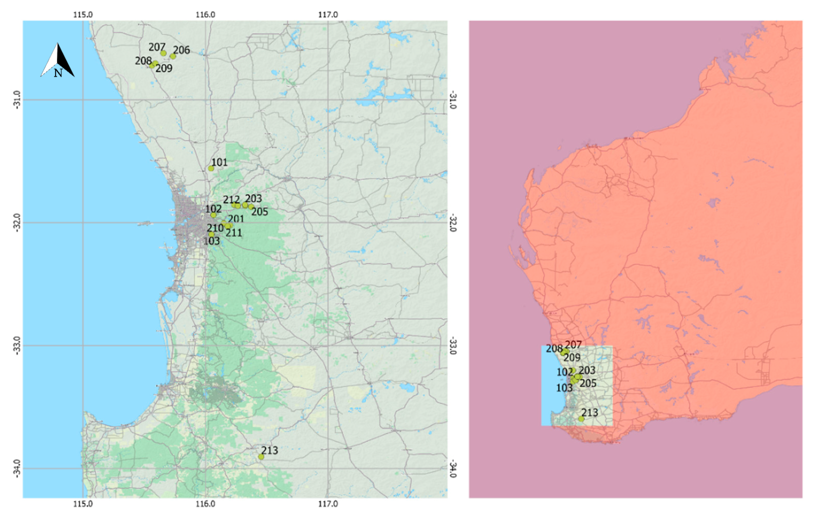
While most apiary sites were within 65 km of the capital city of Perth (Western Australia, −31.95 latitude 115.86 longitude), sites extended from as far north as Dandaragan (140 km north of Perth, −30.66 latitude 115.70 longitude) to as far south as Boyup Brook (230 km south-east of Perth, −33.83 latitude 116.38 longitude). The locations of the apiary sites are shown in
Figure 2. All sites experience a warm temperate climate zone [
10] and fall within the highly biodiverse South West Australian Floristic Region [
11]. While all sites are within the same broad climatic region, the geographic extent of the sites means there is a range of annual weather trends within the study area, with the sites north of Perth being hotter and drier and the site south of Perth being cooler and drier (further inland than Perth). The mean annual and summer weather statistics for the three main areas are summarised in
Table 2.
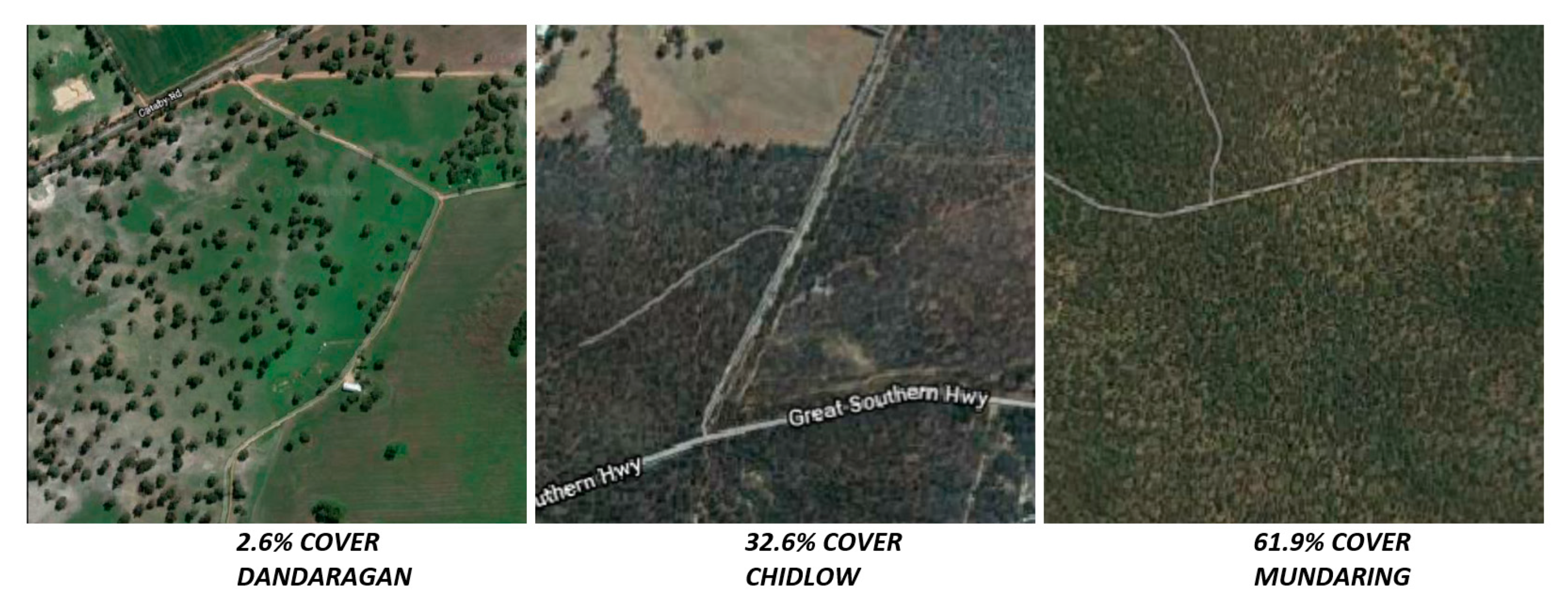
There was also a large range of mature tree canopy cover across the sites. Using the vegetation structure products produced by Auscover [
12] in combination with the height range of mature, flowering
Corymbia calophylla (marri) trees of 10–40 m [
13], the percentage of mature canopy cover for the apiary sites ranges from as low as 2.6% (for a farm site near Dandaragan) to as high as 61.9% (for a forest site in the Beelu National Park, near Mundaring) with a median mature canopy cover of 32.6%. Examples of these canopy cover extents are shown in
Figure 3.
2.2. Temperature, Rainfall and Solar Exposure Datasets
These standard meteorological datasets were retrieved from the Bureau of Meteorology (BOM)’s Australian Data Archive for Meteorology (ADAM), a database that holds weather observations dating back to the mid-1800s for some sites [
14]. Daily weather observations stored within ADAM are readily accessible online via BOM’s Climate Data Online portal [
15]. Weather stations managed by BOM are installed and operated to consistent standards [
16], providing a high degree of confidence when comparing data between years and sites.
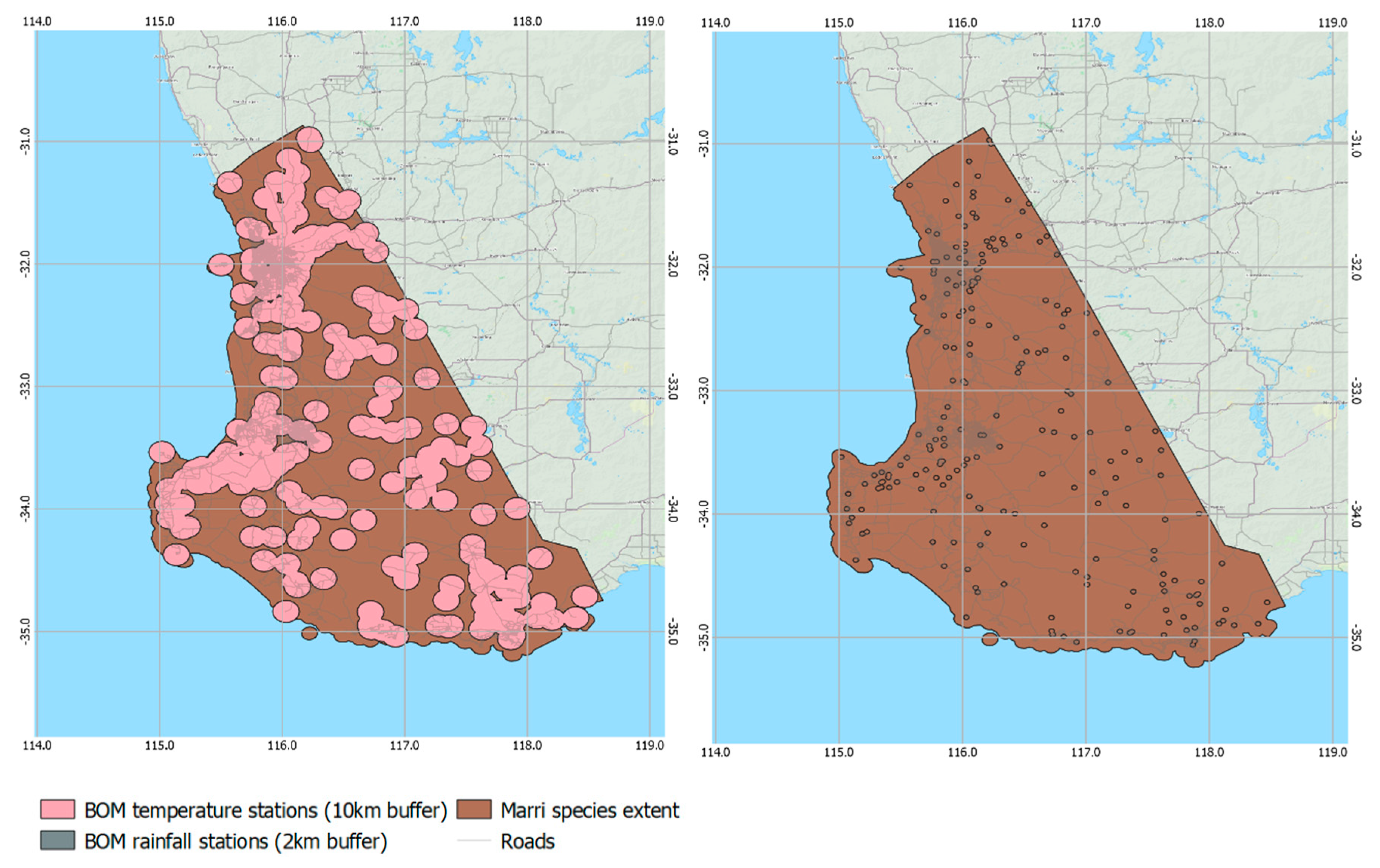
While the individual weather station measurements have a high degree of confidence, weather stations in the study area are widely spaced, with up to 38.9 km between apiary sites and the nearest weather station (
Table 3). With the majority of the surveyed extent of the marri trees covering ~84,000 km
2 [
3], only ~11,000 km
2 (or 13% of this area) has a temperature station within 10 km. This is shown spatially in
Figure 4. The relatively sparse weather station network means that the extrapolation of temperature data to apiary sites may introduce some errors. Additionally, while a 10 km buffer from the rainfall recording stations covers 50% of the surveyed extent of marri trees, the spatial extent of rainfall events, particularly summer thunderstorms, can be much less.
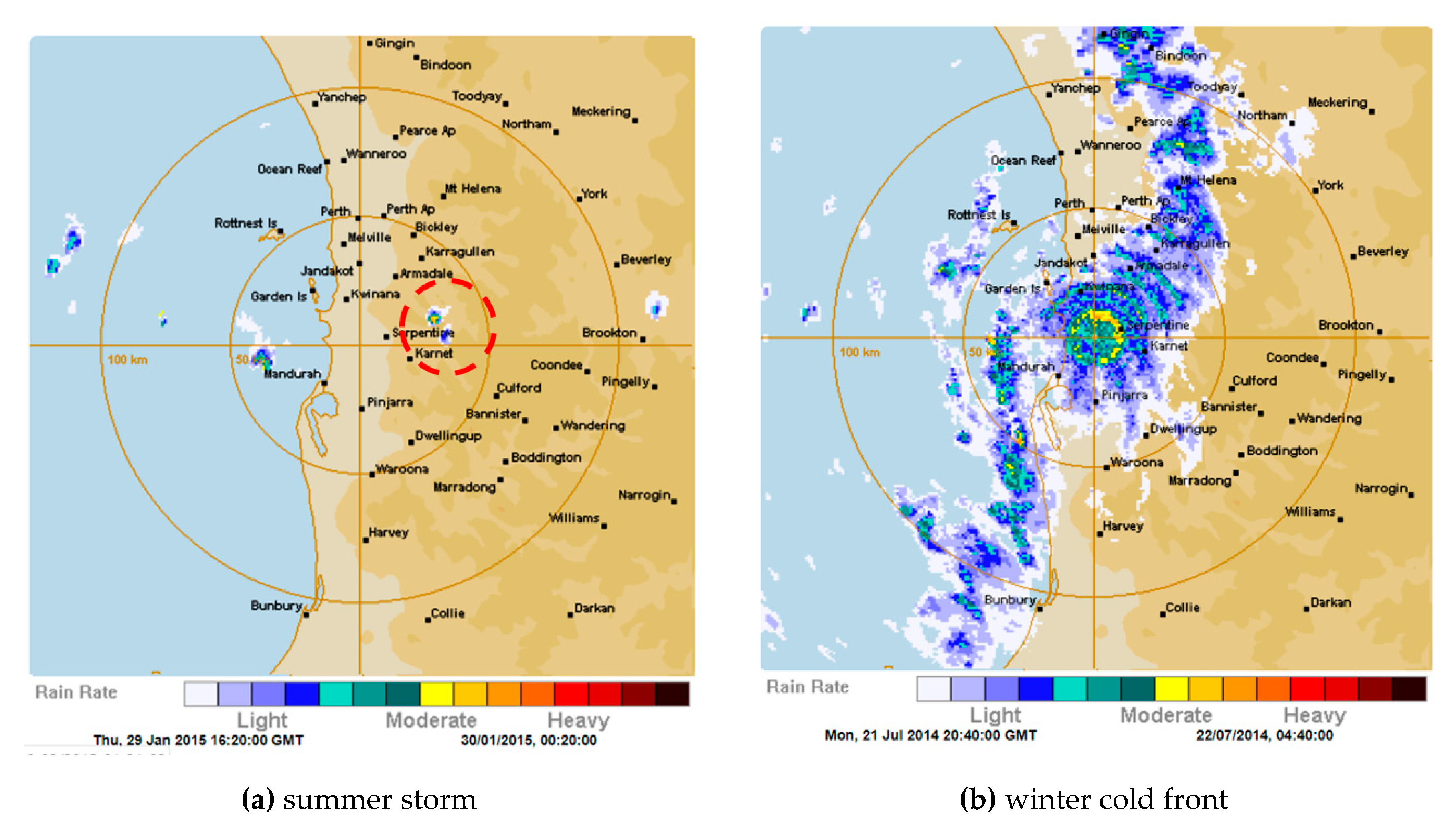
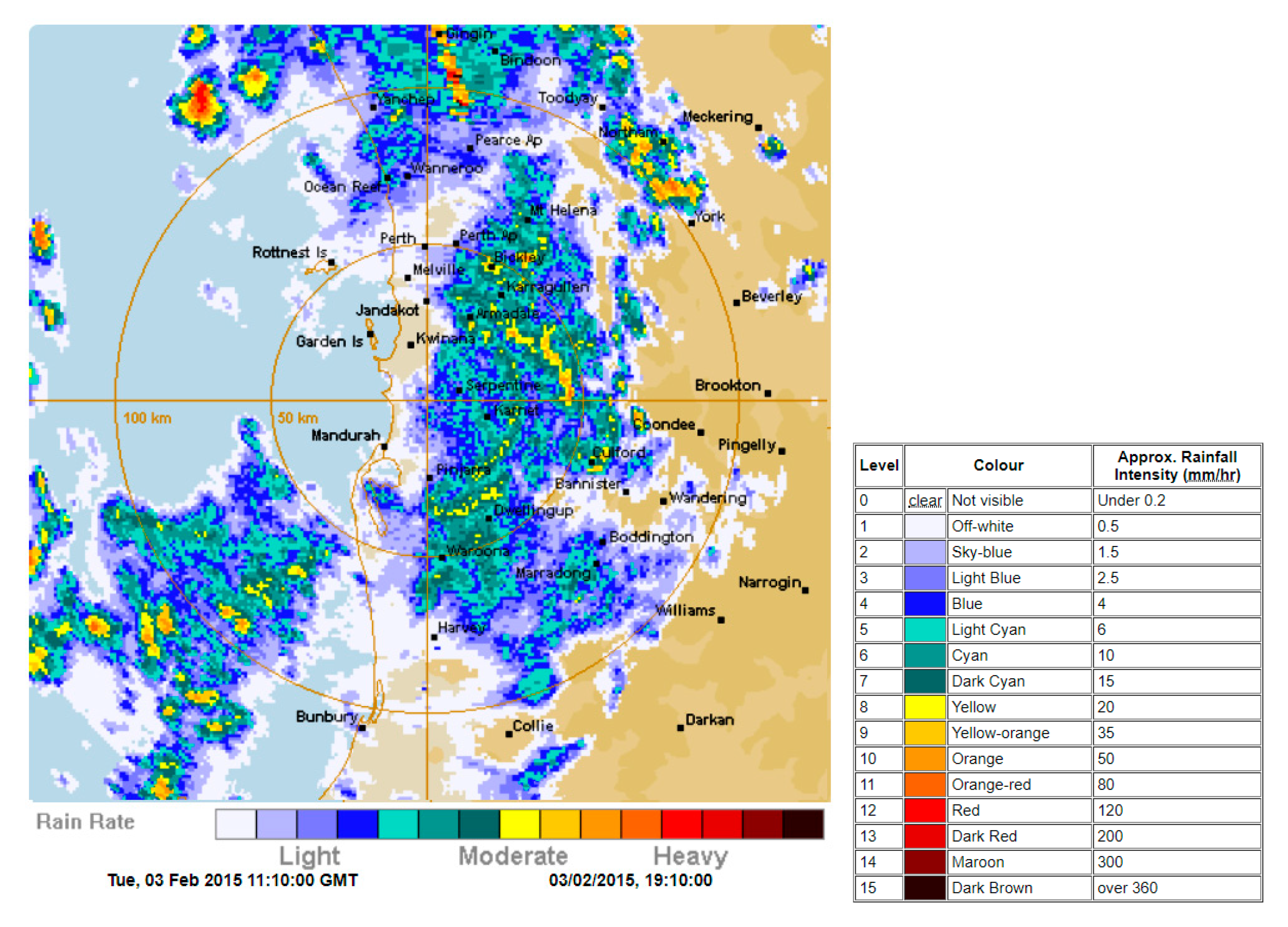
An example of the rainfall from such a storm event is shown in
Figure 5. The main storm feature is approximately 18 km across its long axis but the more intense central area, where rainfall may be as high as 200 mm/h in this case, is just over 2 km across. Reducing the buffer around the BOM rainfall stations to 2 km means that only 3.1% of the marri spatial extent is sufficiently close to a rainfall station to reliably detect these isolated, yet intense, summer rain events. With summer rainfall being one of the key indicators of marri honey harvest weight [
9], this lack of coverage may limit the ability of the BOM rainfall data to reliably classify or predict honey harvest weight.
The distances between the apiary sites where the honey harvest data is from and the nearest weather stations are provided in
Table 3, with temperature stations more than 10 km away and rainfall stations greater than 2 km away highlighted. A total of 75% of the apiary sites are more than 10 km from the nearest temperature station and 75% of the apiary sites are more than 2 km from the nearest rainfall station. Only one apiary site was within both 10 km of a temperature station and 2 km of a rainfall station.
2.3. Satellite-Derived Data
All other input datasets for modelling were derived from the Moderate Resolution Imaging Spectrometer (MODIS) sensor which is carried on the Terra and Aqua satellites [
19], with data retrieved from the Application for Extracting and Exploring Analysis Ready Samples (AppEEARS) online portal [
20]. A summary of the scientific basis for the creation of these datasets follows below. All datasets were retrieved from the AppEEARS portal at a pixel size of 1000 × 1000 m, from the pixel in which the apiary site is located. Retrieving data from coincident pixels meant that the subsequent integration of the data into a single database was a straightforward process. This pixel size was selected based on the typical forage range for honeybees with moderate nectar availability being 1–2 km [
21]. This spatial resolution scale is also in line with studies elsewhere in the world investigating links between honeybee foraging and satellite data, such as eastern Australia [
6] and Europe [
22]. These studies concluded that, due to the foraging distances, the larger pixels of MODIS datasets were a more accurate representation of the foraging conditions for a given apiary site than data from sensors with a higher spatial resolution.
All satellite derived data sets were filtered using the quality control channel contained in the AppEEARS download files. The particulars of the quality control parameters for each dataset can be found in the references provided in the following paragraphs. The quality control filter was set to only allow the highest quality data through into the machine learning algorithm input dataset.
The Gross Primary Production (GPP) MODIS-derived product was developed by Running and Nemani [
23], based on the theory that productivity of crops with sufficient water and nutrient availability is linearly related to the amount of absorbed solar radiation and the efficiency of its use [
24]. The MOD17 data product [
25] used for this study incorporates the vegetation conversion efficiency factor (ε), as well as the effect of water stress and cold conditions on this conversion factor. Ground-based validation of the MOD17 data by Turner and Ritts [
26] found that MOD17 GPP is responsive to general trends associated with local climate and land use, but tended to overestimate GPP in low productivity areas and underestimate GPP in high production areas.
The MOD16A2 Net Evapotranspiration data product [
27] is based on the retrieval of key parameters of the Penman–Monteith evapotranspiration formula from MODIS data [
28]. A reliability study of this data product in dry, heterogenous forests against ground measurements yielded a strong correlation of r
2 = 0.82 [
29], indicating the high overall reliability of the product.
The Normalized Difference Vegetation Index (NDVI) and Enhanced Vegetation Index (EVI) were both retrieved from the MOD13Q1 data product [
30]. NDVI has been found to be strongly related to leaf chlorophyll content, whereas EVI is more indicative of canopy structural variations, including leaf area index (LAI) [
31].
The Marri Flowering Index (MFI), developed by Campbell and Fearns [
32], was designed for direct detection of marri flowers from MODIS data, based on an analysis of spectroradiometer surveys of this particular species. While the MFI has proven to be an effective index for classifying the marri honey harvest weight for some apiary sites with a high proportion of canopy cover [
32], it appears to be less reliable across multiple apiary sites and years [
9].
The Normalised Difference Water Index (NWDI) [
33] is sensitive to changes in the liquid water content of vegetation canopies. This is a proven metric for vegetation water stress [
34], which may impact bud development and nectar production.
2.4. Classification and Regression Tree Analysis
Classification and regression trees [
35] are machine learning methods commonly used to build predictive models from input data [
36]. Both methods partition the input dataset into smaller subsets and perform a simple prediction for each subset. By repeating this process over the entire dataset and combining the simple predictions together, a ‘tree’ type classification or regression structure is made. Classification trees are used for predictive models based on discreet classes or values, while regression trees are used for continuous variables or ranges.
To develop a predictive model, we tested two kinds of regression and classification approaches. Boosted Regression Trees (BRTs) are versatile, tree-based regression methods that can handle input features of different data types, while handling complex nonlinear relationships as well as interaction effects between the input features [
37]. Random Forest trees have become popular in recent years for remote sensing and ecological applications due to their ability to handle both high data dimensionality and multicollinearity, which are common in multi-spectral remote sensing data, and the fact that they are both fast and insensitive to overfitting [
38]. The Scikit-learn code for Python was used for the analysis [
39], with the
GradientBoostingRegressor,
GradientBoostingClassifier,
RandomForestRegressor and
RandomForestClassifier functions initially used to assess which approach resulted in the most accurate predictive model.
2.5. Results
Input data were retrieved from several different sources for periods both preceding and during the main honey flow period for marri trees (February). The sources, periods and abbreviations used hereafter for these data are provided in
Table 4. In total, a multidimensional database of 115 input features was created from the data summarised in
Table 4.
To assess the predictive accuracy of each algorithm, both the regression and classifier functions for the gradient boosted and Random Forest tree algorithms were run for all 115 input features, with an increasing number of trees in the model. No complexity limit was given due to the relatively small size of the dataset and the resulting short run time. The output from this testing (see
Table 5) shows that the Random Forest functions worked better for the classification approach, based on the ‘poor year’, ‘moderate year’ and ‘good year’ ratings, and the Gradient Boosted functions worked better for predicting the honey harvest weights via the regression model.
The lowest predictive errors came from the use of Gradient Boosted Regression (GBR), with a mean average error of +/− 10.3 kg for the weight, with this weight being in the correct class 82% of the time.
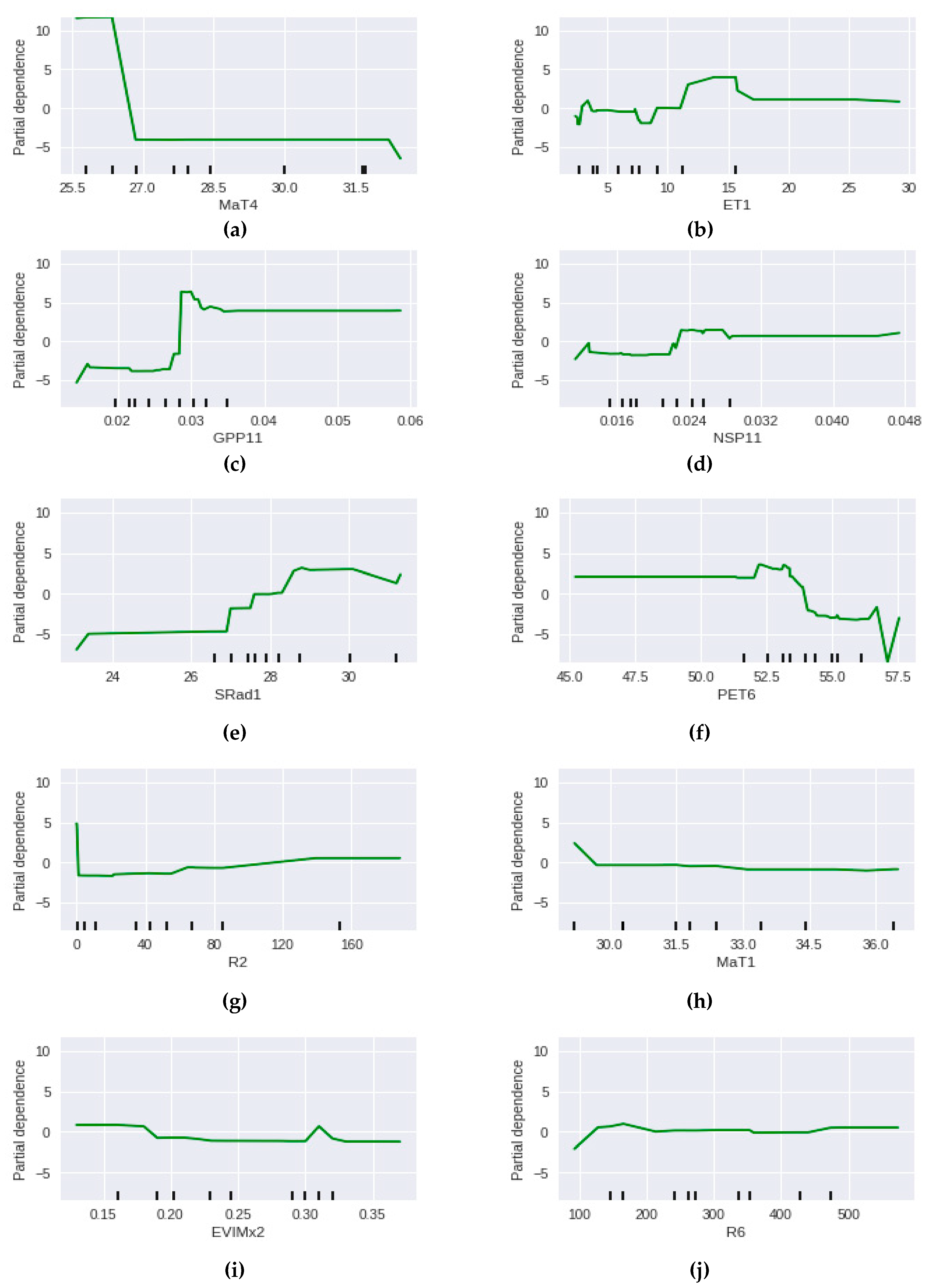
The partial dependence plots for the 10 features with the highest feature importance from the full feature input model are shown in
Figure 6. These plots show that the model predictions have the highest dependence on the mean maximum temperature for October–January (MaT4), with mean maximum temperatures below 27 °C having a strong positive relationship and mean maximum temperatures above 27 °C having a negative relationship. There are also strong relationships with Gross Primary Production from the 11 months preceding the flowering period (GPP11), with low GPP associated with lower honey production, and a higher evapotranspiration for January (ET1) having a positive relationship with higher honey production.
In order to determine whether the dimensionality of the input features could be reduced without compromising the predictive accuracy of our models, the GBR function was run multiple times with fewer input features for each run. The selection of input features for each run was on the basis of the highest feature importance from the preceding model.
Table 6 shows the VIs and predictive errors for this process. The MaT4 feature is clearly the most important input, with a VI of 37.7% even when all 115 features are used in the regression modelling. This is followed by ET1 and GPP, both at below 10% when all feature inputs are used. The columns highlighted in green show the models with the lowest error, by class (five input features) and by weight (two input features). These reduced input feature models both have slightly higher honey weight prediction errors than the full feature model (increased error of 0.52 kg versus a honey harvest range of 0.0 kg to 71.0 kg in the training and testing datasets). If this simplified approach were to be applied to larger datasets for the prediction of honey harvest weight, a significantly smaller number of feature inputs can be used, with a minimal reduction in predictive accuracy, reducing the size of the multidimensional dataset required.
The ‘Honey class. (1–2)’ row in
Table 6 is calculated by classifying the predicted honey weight as either ‘good year’ or ‘below good year’, based on the high degree of clustering found with key weather and satellite inputs for ‘good years’ by Campbell and Fearns [
9]. This tight clustering for ‘good years’, and the 0% error in the predictive regression classification, means that for this dataset the ‘good year’ prediction is both an accurate and a robust model. While this cannot assist apiarists with preparation for ‘poor years’, when their bees can sometimes starve due to the lack of nectar, the apiarists can prepare for a ‘good year’ in advance and therefore increase the honey production, compared with being unprepared for a ‘good year’ and having insufficient hives or other equipment to facilitate efficient use of the abundant resource.
Although the predictive regression model developed solely from the MaT4 and ET1 features has a relatively low error and is shown to be quite robust at predicting harvests that are ‘good years’, both input features require data from the month immediately preceding the honey flow. If the predictive model developed here was used operationally by beekeepers to adaptively manage their beehives, this timing of the key input data would limit the time available for apiarists to prepare for a ‘good year’. To determine whether a predictive model could be generated with a longer lead time into the honey flow, mean maximum temperatures for the individual months from October to January were also tested in the GBR, as well as combinations of these months. The VIs from this process are summarised in
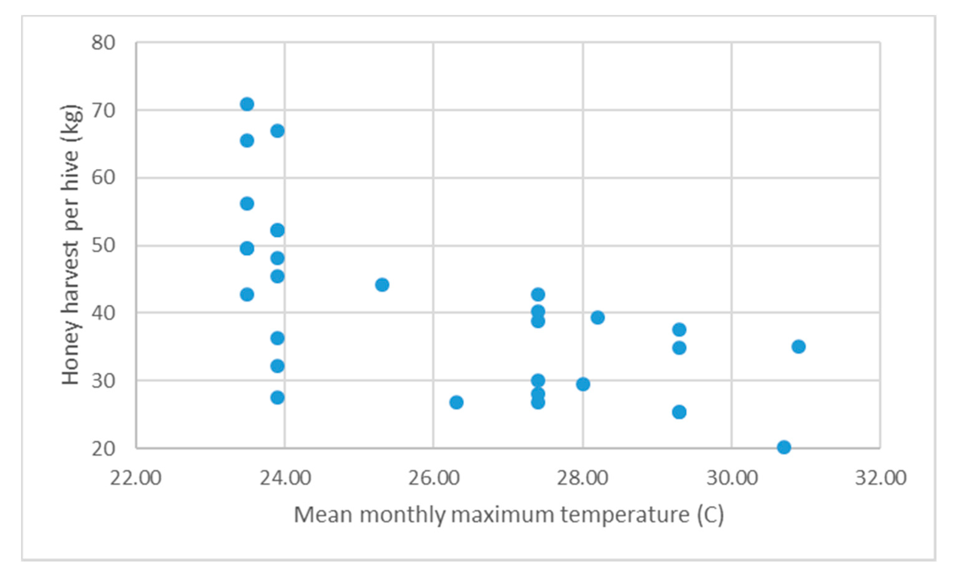
Table 7. While the original MaT4 and ET1 features retained a high importance, MaT3 (mean maximum temperature for November) was also assessed as a key feature input, based on a visual assessment of the clustering of each feature versus honey harvest weight (see
Figure 7). While the model does not produce the lowest errors, it is nonetheless a reliable predictor (particularly for ‘good years’ versus non-good years). The lower accuracy of the prediction is offset by the lead time to the honey flow; with honey flow generally starting in late January to early February [
32], having a strong indicator of an upcoming good harvest by the end of November gives apiarists approximately two months to prepare for the predicted conditions.
3. Discussion
From the regression tree analysis performed in this study, there are a range of different factors that influence the honey harvest of marri trees and the timeframe of some of these factors (e.g., Gross Primary Productivity) can be as much as a year before the honey flow starts. Despite the range of available input variables that we explored, we found that the inputs to the predictive model can be reduced significantly with a minimal reduction in the accuracy of the predictive model. The mean maximum temperature for the few months preceding honey flow (November to January) and the evapotranspiration in the month before honey flow (January) were found to describe the majority of the variability in honey harvest weight almost as accurately as the full multidimensional dataset of 115 input features.
The potential limitations in the accuracy of the weather station data available from BOM, due to the sparsity of stations across the extent of marri trees versus the spatial variability of the observations, may mean that some relationships between marri honey production and weather may not be fully captured in the existing database. The sparse nature of rainfall stations compared to the localised nature of summer rainfall events means that the influence of rainfall in particular may have been poorly characterised in our input dataset. Unfortunately, due to this sparsity of rainfall stations, excluding apiary sites from the database that have temperature stations more than 10 km away and/or rainfall stations more than 2 km away would result in only one apiary site in the database with honey harvests from two of the study years. This is insufficient data for the development of a predictive model, particularly as both of these years are ‘good years’ (>40 kg of marri honey per hive).
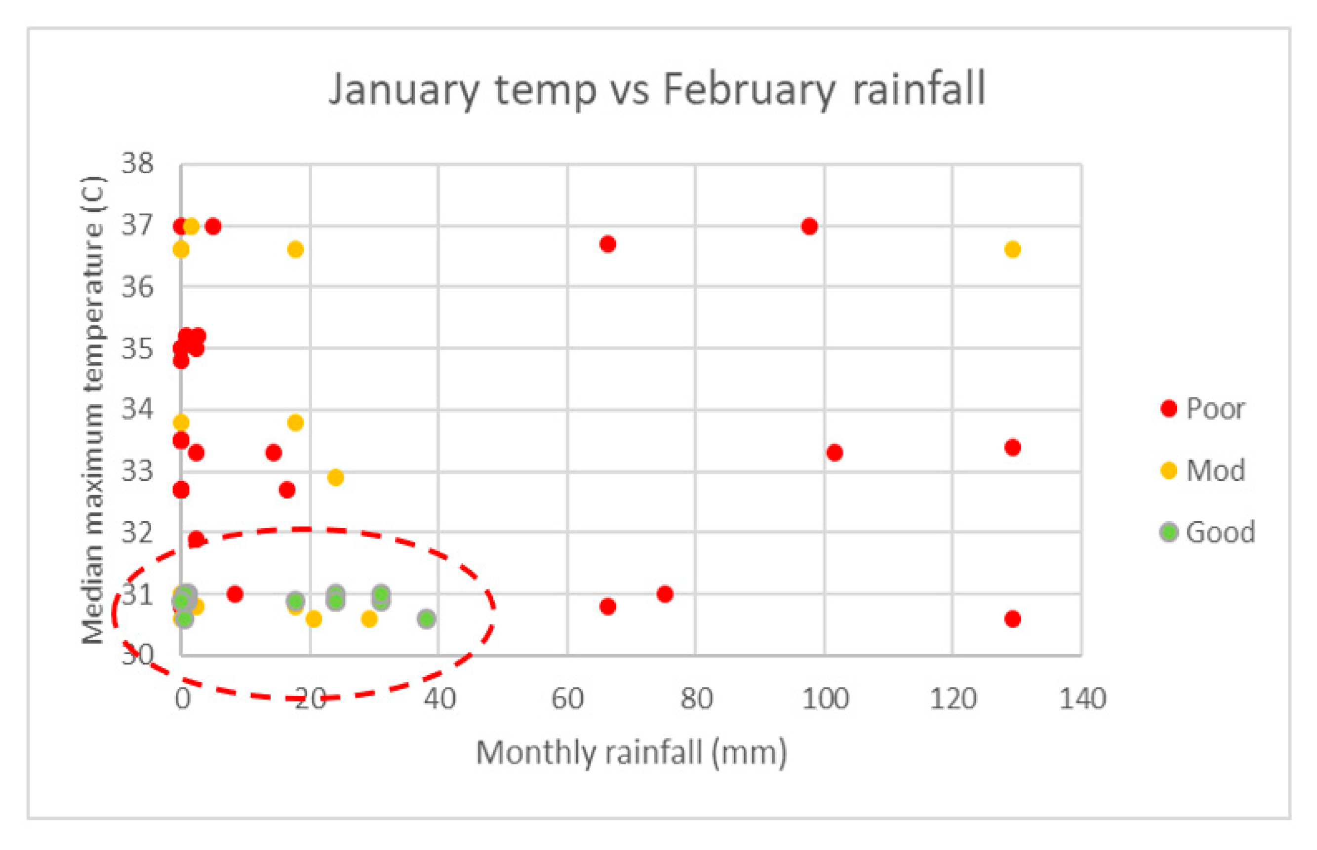
Rainfall immediately preceding and during the flowering period is one of the key factors in harvest quality (see
Figure 8), with heavy summer rainfall events after flowering commences actually knocking stamen, and sometimes flowers, from the trees [
40]. This presents an issue with the development of a predictive model as, even with good conditions in the lead up to the peak flowering period, a localised storm may downgrade a prospective harvest from a ‘good year’ to a ‘moderate year’ or even a ‘poor year’ in a matter of hours.
Such a localised storm may have been the cause of the quality of some of the ‘moderate year’ harvests in the Perth Hills in 2015 being incorrectly classified as ‘good years’ by the predictive model; the November mean maximum temperature was within the range for a good harvest that season, but three of the eight apiary sites only yielded a harvest that was a ‘moderate year’. Rainfall for all of the apiary sites was below 40 mm for February (in the range 18.6–30.0 mm). The rainfall radar image from the main rainfall event at the start of the month, shown in
Figure 9, contains localised patches of more intense rainfall (up to 80 mm/hr) that are under 2 km across. The presence of one of these localised higher intensity zones over an apiary site may well have increased the rainfall received by the site to over 40 mm for the period, the upper limit for good harvests from the currently available data [
9].
With marri honey being the largest annual honey harvest in Western Australia [
42], the highly specific conditions required for a good harvest may be less likely to occur with the projected climate models for the extent to which marri trees occur. The Regional Climate Model developed for southwest Western Australia by Andrys and Kala [
42] assessed projections of both mean and extreme weather events over the period from 2030 to 2059 under a high greenhouse gas emissions scenario. Compared with historic data from 1970 to 1999, mean maximum temperatures for spring and summer are projected to increase by between 0.5–2.0 °C. With more than 80% of the ‘good years’ occurring in seasons where the preceding November mean maximum temperature is less than 24.0 °C. As the November mean maximum temperature for the Perth Hills region is already at 25.0 °C, the probability of this criteria for a good harvest being met will likely decrease. In addition, while the projections for summer rainfall vary considerably between models, the models all predict that the intensity of summer rainfall events will increase, resulting in an increase in the probability of localised rainfall events of sufficient intensity to reduce the harvest quality.
4. Conclusions
The development of a multidimensional database with 115 factors that may influence the honey production of marri trees was subjected to a regression tree analysis. The GBR models achieved the highest predictive accuracy when all features from the multi-dimensional dataset were used, with an average error of +/− 10.33 kg for the weight, with the weight being in the correct class 82% of the time. A similar level of predictive accuracy was achieved with a revised GBR model using the input features with the five highest values of feature importance. This regression model was able to predict the honey yield per hive with a mean average error (MAE) of 10.85 kg and classify the harvest into the correct quality category with 92% accuracy.
Analysis of the predictive accuracy of GBRs with different input features highlighted that ‘good years’ could be predicted robustly compared with ‘moderate years’ and ‘poor years’ (100% accuracy with only one or two input features in the models). With mean maximum temperature in the months leading up to the marri honey flow consistently rating among the highest importance values, testing the model with various combinations found that using the November mean maximum temperature on as the only input feature into the GBR algorithm could predict the honey harvest weight per hive to an MAE of 11.72 kg, classify it into the correct class with 75% accuracy and predict a ‘good year’, versus other types of year, to 100% accuracy. With the honey flow typically starting in February, giving apiarists a reliable predictor of a good season two months ahead of time will allow them to prepare their equipment, including establishing new hives, before the flow starts to improve the production in years with good honey harvests.
In an operational setting, the accuracy of the prediction models may be restricted by the availability of weather data, with less than 13% of the extent of marri trees having a temperature station within 10 km. Intense localised summer rainfall events also have an important role to play in making the model more widely applicable. Only 3.1% of the marri areas have a rainfall station within 2 km. Access to more spatially accurate weather data may be able to improve the regression model’s predictive accuracy.
With cooler weather and lower summer rainfall required for good marri honey harvests, the climate projections for southwest Western Australia indicate that good harvests are likely to become rarer in the future, with mean maximum temperatures and the intensity of summer rainfall both projected to increase.
While this study has been focused on honey production from a single species endemic to South West Australia, the weather stations and satellite data used to develop the model, for example, the Royal Netherlands Meteorological Institute (KNMI) Climate Explorer tool [
43], have collected over 10 TB of weather data from multiple weather agencies around the world (including the BOM data used for this study). The MODIS input feature data are freely available global datasets produced by NASA. If these data are used in conjunction with honey harvest data from other species and/or regions, predictive models could foreseeably be developed using the methodology employed for in study for other honey harvests.
Author Contributions
Conceptualization, T.C. and P.F.; methodology, T.C.; investigation, T.C.; writing-original draft preparation, T.C.; writing-review and editing, K.W.D., K.D., P.F. and R.H.; funding acquisition, K.D. All authors have read and agreed to the published version of the manuscript.
Funding
This research is supported by the Beekeeping Industry Council of Western Australia (BICWA), the Western Australian government’s Department of Primary Industries and Regional Development (DPIRD) and ChemCentre as part of the Grower Groups Research and Development Grant, Round 2-GGRD2 2016-1700179-INDUSTRY STANDARDS OPTIMISING STORAGE AND SUPPLY VOLUME OF WA MONO-FLORAL HONEY.
Conflicts of Interest
The authors declare no conflict of interest. The funders had no role in the design of the study; in the collection, analyses, or interpretation of data; in the writing of the manuscript, or in the decision to publish the results.
References
- Thomson, J. Western Australia a Sweet Spot for Beekeeping; Department of Primary Industries and Regional Development: Perth, Australia, 2019.
- Irish, J.; Blair, S.; Carter, D. The Antibacterial Activity of Honey Derived from Australian Flora. PLoS ONE 2011, 6, e18229. [Google Scholar] [CrossRef]
- Herbarium, W.A. Florabase—the Western Australian Flora; Department of Environment and Conservation: Perth, Australia, 1998.
- Hudson, I.L.; Kim, S.; Keatley, M. Climatic influences on the flowering phenology of four Eucalypts: A GAMLSS approach. In Proceedings of the 18th World IMACS Congress and MODSIM09 International Congress on Modelling and Simulation, Cairns, Australia, 13–17 July 2009. [Google Scholar]
- Arundel, J.; Winter, S.; Gui, G.; Keatley, M. A web-based application for beekeepers to visualise patterns of growth in floral resources using MODIS data. Environ. Model. Softw. 2016, 83, 116–125. [Google Scholar] [CrossRef]
- Webber, E. Eucalypt Leaf-Flush Detection from Remotely Sensed (MODIS) Data; Department of Infrastructure Engineering-Geomatics, University of Melbourne: Melbourne, Australia, 2011. [Google Scholar]
- Winter, S.; Leach, J.; Keatley, M.; Arundel, J. BeeBox Application User Manual; Burns, C., Ed.; Rural Industries Research and Development Corporation: Canberra, Australia, 2013. [Google Scholar]
- Hawkins, B.; Thomson, J.; Mac Nally, R. Regional patterns of nectar availability in subtropical eastern Australia. Landsc. Ecol. 2018, 33, 999–1012. [Google Scholar] [CrossRef]
- Campbell, T.; Fearns, P.; Dods, K.; Dixon, K. Prediction and detection of honey harvests from remote sensing and weather data. Int. J. Eng. Sci. Res. Technol. 2019, 8, 7–88. [Google Scholar]
- Peel, M.C.; Finlayson, B.L.; Mcmahon, T.A. Updated world map of the Köppen-Geiger climate classification. Hydrol. Earth Syst. Sci. Discuss. 2007, 4, 439–473. [Google Scholar] [CrossRef] [Green Version]
- Beard, J. A New Phytogeographic Map of Western Australia; Western Australian Herbarium Research Notes; Western Australian Herbarium: Kensington, Australia, 1980; Volume 3, pp. 37–58. [Google Scholar]
- Scarth, P. Vegetation Height and Structure—Derived from ALOS-1 PALSAR, Landsat and ICESat/GLAS, Australia Coverage; Phinn, S., Ed.; Joint Remote Sensing Research Program, University of Queensland: Brisbane, Australia, 2009. [Google Scholar]
- Brooker, M.I.H.; Kleinig, D.A. Field guide to eucalypts. In South-western and Southern Australia; Bloomings Books: Melbourne, Australia, 2001; Volume 2. [Google Scholar]
- Meteorology, B.O. (Ed.) Australian Data Archive for Meteorology. In Conference on Managing Australian Climate Variability; NSW: Albury, Australia, 2000. [Google Scholar]
- Bureau of Meteorology. Climate Data Online. Available online: http://www.bom.gov.au/climate/data (accessed on 21 April 2019).
- Canterford, R. Guidelines for the Siting and Exposure of Meterological Instruments and Observing Facilities; Bureau of Meteorology, Department of the Environment, Sports and Territories: Melbourne, Australia, 1997. [Google Scholar]
- Bureau of Meteorology. Weather Station Directory. Available online: http://www.bom.gov.au/climate/data/stations/ (accessed on 8 February 2019).
- The Weather Chaser. Perth Radar—128km Rain Rate. Available online: http://www.theweatherchaser.com/radar-loop/IDR703-perth-serpentine (accessed on 21 March 2019).
- Barnes, W.L.; Pagano, T.S.; Salomonson, V.V. Prelaunch characteristics of the moderate resolution imaging spectroradiometer (MODIS) on EOS-AMI. IEEE Trans. Geosci. Remote Sens. 1998, 36, 1088–1100. [Google Scholar] [CrossRef] [Green Version]
- AppEEARS Team. Application for Extracting and Exploring Analysis Ready Samples (AppEEARS). NASA EOSDIS Land Processes Distributed Active Archive Center (LP DAAC), USGS/Earth Resources Observation and Science (EROS) Center: Sioux Falls, SD, USA. Available online: https://lpdaacsvc.cr.usgs.gov/appeears/ (accessed on 12 March 2019).
- Hagler, J.R.; Mueller, S.; Teuber, L.R.; Machtley, S.A.; Van Deynze, A. Foraging range of honey bees, Apis mellifera, in alfalfa seed production fields. J. Insect Sci. 2011, 11, 144. [Google Scholar] [CrossRef] [PubMed] [Green Version]
- Lynn, B.C. Relation of Honey Production in Apis Mellifera Colonies to the Normalized Difference Vegetation Index and Other Indicators. Ph.D. Thesis, Department of Geography, University of North Carolina, Chapel Hill, NC, USA, 2013. [Google Scholar]
- Running, S.W.; Nemani, R.R.; Heinsch, F.A.; Zhao, M.; Reeves, M.; Hashimoto, H. A Continuous Satellite-Derived Measure of Global Terrestrial Primary Production. BioScience 2004, 54, 547–560. [Google Scholar] [CrossRef]
- Monteith, J.L. Solar Radiation and Productivity in Tropical Ecosystems. J. Appl. Ecol. 1972, 9, 747–766. [Google Scholar] [CrossRef] [Green Version]
- Running, S.W.; Mu, Q.; Zhao, M. MOD17A2H MODIS/Terra Gross Primary Productivity 8-Day L4 Global 500m SIN Grid V006; NASA EOSDIS Land Processes DAAC, 2015. Available online: https://lpdaac.usgs.gov/products/mod17a2hv006/ (accessed on 24 March 2019).
- Turner, D.P.; Ritts, W.D.; Cohen, W.B.; Gower, S.T.; Running, S.W.; Zhao, M.; Costa, M.H.; Kirschbaum, A.A.; Ham, J.M.; Saleska, S.R.; et al. Evaluation of MODIS NPP and GPP products across multiple biomes. Remote Sens. Environ. 2006, 102, 282–292. [Google Scholar] [CrossRef]
- Running, S.W.; Mu, Q.; Zhao, M. MOD16A2 MODIS/Terra Net Evapotranspiration 8-Day L4 Global 500m SIN Grid V006; NASA EOSDIS Land Processes DAAC, 2017. Available online: https://lpdaac.usgs.gov/products/mod16a2v006/ (accessed on 24 March 2019).
- Mu, Q.; Heinsch, F.A.; Zhao, M.; Running, S.W. Development of a global evapotranspiration algorithm based on MODIS and global meteorology data. Remote Sens. Environ. 2007, 111, 519–536. [Google Scholar] [CrossRef]
- Miranda, R.D.Q.; Galvíncio, J.D.; Moura, M.S.B.D.; Jones, C.A.; Srinivasan, R. Reliability of MODIS Evapotranspiration Products for Heterogeneous Dry Forest: A Study Case of Caatinga. Adv. Meteorol. 2017, 2017. [Google Scholar] [CrossRef]
- Didan, K. MOD13Q1 MODIS/Terra Vegetation Indices 16-Day L3 Global 250m SIN Grid V006; NASA EOSDIS Land Processes DAAC, 2015. Available online: https://lpdaac.usgs.gov/products/mod13q1v006/ (accessed on 24 March 2019).
- Schnur, M.T.; Xie, H.; Wang, X. Estimating root zone soil moisture at distant sites using MODIS NDVI and EVI in a semi-arid region of southwestern USA. Ecol. Inform. 2010, 5, 400–409. [Google Scholar] [CrossRef]
- Campbell, T.; Fearns, P. Honey crop estimation from space: Detection of large flowering events in Western Australian forests, in ISPRS TC I Mid-term Symposium “Innovative Sensing—From Sensors to Methods and Applications”. In Proceedings of the 2018 International Society for Photogrammetry and Remote Sensing, Karlsruhe, Germany, 4–5 October 2018; pp. 79–86. [Google Scholar]
- Gao, B.-C. NDWI A Normalized Difference Water Index for Remote Sensing of Vegetation Liquid Water From Space. Remote Sens. Environ. 1996, 58, 257–266. [Google Scholar] [CrossRef]
- Clay, D.E.; Kim, K.I.; Chang, J.; Clay, S.A.; Dalsted, K. Characterizing Water and Nitrogen Stress in Corn Using Remote Sensing. Charact. Water Nitrogen Stress Corn Using Remote Sens. 2006, 98, 579–587. [Google Scholar] [CrossRef]
- Breiman, L. Classification and Regression Trees; Wadsworth International Group: Belmont, CA, USA, 1984. [Google Scholar]
- Loh, W.-Y. Classification and Regression Trees. Wiley Interdiscip. Rev. Data Min. Knowl. Discov. 2011, 1, 14–23. [Google Scholar] [CrossRef]
- Elith, J.; Leathwick, J.R.; Hastie, T. A working guide to boosted regression trees. J. Anim. Ecol. 2008, 77, 802–813. [Google Scholar] [CrossRef] [PubMed]
- Belgiu, M.; Drăguţ, L. Random forest in remote sensing: A review of applications and future directions. ISPRS J. Photogramm. Remote Sens. 2016, 114, 24–31. [Google Scholar] [CrossRef]
- Pedregosa, F.; Varoquaux, G.; Gramfort, A.; Michel, V.; Thirion, B.; Grisel, O.; Vanderplas, J. Scikit-learn: Machine Learning in Python. J. Mach. Learn. Res. 2011, 12, 2825–2830. [Google Scholar]
- Leyland, D. Review of Historic Marri Harvest Records; Personnal communication: Chidlow, Australia, 2015. [Google Scholar]
- Painter, S. Jarrah Honey Crisis as Yield Wiped out, in The West Australian; Seven West Media: Perth, Australia, 2010. [Google Scholar]
- Andrys, J.; Kala, J.; Lyons, T. Regional climate projections of mean and extreme climate for the southwest of Western Australia (1970–1999 compared to 2030–2059). Obs. Theor. Comput. Res. Clim. Syst. 2017, 48, 1723–1747. [Google Scholar] [CrossRef]
- Oldenborgh, G. Climate Explorer: Starting Point. Available online: http://climexp.knmi.nl/start.cgi (accessed on 4 April 2019).
© 2020 by the authors. Licensee MDPI, Basel, Switzerland. This article is an open access article distributed under the terms and conditions of the Creative Commons Attribution (CC BY) license (http://creativecommons.org/licenses/by/4.0/).


