Identification of the Conditions for Organic Agriculture Development in Polish Districts—An Implementation of Canonical Analysis

Abstract

Organic farming in Poland has been developing dynamically since the accession to the EU. However, there are considerable differences in the level of organic farming development in particular regions. Therefore, it is vital to identify the primary factors and conditions for this development and their importance considering their spatial distribution. The presented paper aims to estimate the relationships between the level of organic agriculture development and selected conditions of financial and environmental character. The investigation is based on primary data for 2017 retrieved from the Local Data Bank of the Main Statistical Office and Agricultural and Food Quality Inspection database for all Poland districts. In order to achieve this objective, a multivariate statistical analysis method—the canonical correlation was applied. The analysis was preceded by constructing the composite indices of organic agriculture development and its conditions based on a Technique for Order of Preference by Similarity to Ideal Solution (TOPSIS) method and correlation analysis between the indices developed by the authors. The performed canonical analysis showed two statistically significant canonical variables with relatively high values of the canonical correlation (0.74 and 0.59). It proves that the degree of explaining the variability of one set of variables through linear relationships (referring to the level of organic farming development), by the second input data set (describing the determinants of the development), by successive pairs of canonical variables is high. This means that the created model describes relatively well the considered data sets.

1. Introduction

The dynamic development of organic agriculture in Europe, observed for several decades, deserves special attention among new food economy occurrences. The reasons for this phenomenon may be found in the growing chemization of non-organic agriculture and food processing, followed by the increase of consumers’ health and environmental awareness [1,2]. However, in Poland, this development could not start before 1989 because of the prevailing political system and centrally managed economy.

Organic farming is believed to have the potential to solve particular contemporary problems by bringing benefits in environmental protection and preserving non-renewable resources. It also contributes to increasing food quality, reducing surplus goods production, and reorienting agriculture toward places where the market demand occurs [3]. Many researchers defined organic farming. Mannion [4] described the organic production system as a holistic understanding of agriculture that intends to reflect the deep interdependence between farm biota, agricultural production, and the environment. Lampkin and Padel [5] emphasized that the purpose of organic agriculture is the creation of integrated, humane, environmentally, and economically sustainable production systems. That system should maximize dependence on inputs produced within the farm and managing ecological and biological processes and interactions. These ought to lead to the achievement of satisfactory levels of crops, livestock, and human nutrition, protection from pests and disease, and finally, an adequate return to the human and other resources.

According to the International Federation of Organic Agriculture Movements (IFOAM), an umbrella organization in the field of organic agriculture [6], organic farming “is a production system that sustains the health of soils, ecosystems, and people. It relies on ecological processes, biodiversity, and cycles adapted to local conditions, rather than inputs with adverse effects. Organic agriculture combines tradition, innovation, and science to benefit the shared environment and promotes fair relationships and good quality of life for all involved”. MacRae et al. [7] represent a similar approach. According to them, organic methods are in line with natural processes to preserve resources and reduce waste and environmental harm while keeping farms’ economic performance. Therefore, organic agriculture takes maximum advantage of available soil nutrient and water cycles, energy flows, useful soil organisms, and natural pest controls. By benefiting from natural cycles, environmental damage can be reduced. It also provides the humane treatment of animals, the rural population’s well-being, and nutritious food without harmful substances.

Considering the above-cited definitions, one may conclude that organic farming development can significantly contribute to sustainable development [8]. It shares the primary goals of agriculture and may be recognized as a significant part of sustainable farming where natural, economic, and social values are equally treated [9]. As already mentioned, organic farming is also perceived as a potential solution to industrial agriculture problems, such as deteriorating natural resources, worsening food quality, and reduced rural areas’ viability, mostly because it balances multiple sustainability goals [10,11]. It has a positive impact on soil and therefore can improve soil quality. It can increase the soil’s capacity to maintain biological activity and diversity due to avoiding chemical inputs. It may also help achieve adequate fertility and regulate water and filter and buffer inorganic materials and control soil erosion [12,13]. Like other sustainable production systems, organic agriculture limits the application of hormones and antibiotics for animals. Their use is restricted to the cases when it is necessary for animal health and applied in individual treatment. If possible, depending on weather conditions, animals should have permanent access to open pasture and meet their nutritional needs [14]. Conversion to organic agriculture may also be a possible way of reducing energy consumption and greenhouse gas emissions. Synthetic chemicals and fertilizers are substantial sources of energy use, and the conversion to organic agriculture, which is less dependent on these inputs, may decrease these impacts [15,16]. Therefore, environmental aspects refer to the gains in biodiversity, environmental protection, and decreased resource consumption. Considering sustainable development, organic agriculture is based on decentralization, independence, community, harmony with nature, diversity, and restraint. By reducing chemo-synthetic inputs, it decreases to some extent, relatively high production costs resulting from, among other things, labor-consuming practices. Other social aspects involve social relations, political, and cultural development [17,18,19]. Moreover, this method decreases health problems, sustains food security [20], and creates workplaces due to the use of labor-consuming practices [21], which, on the other hand, increases production costs. In terms of promoting human health, organic food is considered to play an important role due to its high nutritional quality and reduction of harmful chemicals [19,22]. In addition, organically raised livestock supports its health and reduces the risk of diseases. Therefore, it can contribute to rural and social capital development as well as local community situation improvement [23].

Therefore, in the early 1990s, at the EU (formerly EEC) level, the regulations on organic farming were elaborated as well as financial support to this farming system was introduced. In 1991, Council Regulation (EEC) No 2092/91 of 24 June 1991 on organic production of agricultural products and indications referring thereto on agricultural products and foodstuffs covering organic production rules, and permitted substances applied in organic agriculture, guidelines for processing, rules for inspection, labeling of organic food, import rules, was adopted [24]. In 1999, Council Regulation (EC) No 1804/1999 of 19 July 1999 supplementing Regulation (EEC) No 2092/91 on organic production of agricultural products and indications referring thereto on agricultural products and foodstuffs to include livestock production was introduced that implemented the voluntary indication of organic food products [25]. The works on the legislation in the area of organic agriculture were further performed to adjust it better to the current situation of organic farming. In 2007, the new Council Regulation (EC) No 834/2007 of 28 June 2007 on organic production and labeling of organic products and repealing Regulation (EEC) No 2092/91 came into force on 1st January 2009 [26], which again after a decade required revision. Therefore, a new regulation was adopted in 2018, which will be applicable in 2021. It generally introduces stricter rules for organic farming practices and processing [27].

In the early 1990s, the instruments directed towards the realization of the aims related to the protection of the natural environment, i.e., agri-environmental programs were launched. They also enabled the implementation of an organic farming support system. The support system is based on the belief that farmers should obtain income not only from agricultural production but also for maintaining the traditional character of rural areas and applying environmentally-friendly production methods. Within agri-environmental programs, subsidies were paid for environmental protection measures, maintenance of natural resources and elements of the village’s cultural heritage. This kind of support covered payments for the area dedicated to particular crops and additional tools such as subsidies for inspection costs, training, or research programs. Its implementation’s direct effect was the growth of the number of organic farms and organic crop areas. Initially, these programs were covered by Regulation 2078/92 [28]. It introduced a wide range of support possibilities in the form of so-called schemes (including organic farming), i.e., different environmental undertakings exceeding the code of good agricultural practice and simultaneously favoring the natural environment and maintaining the countryside landscape.

The implementation of agri-environmental programs enabled the dynamic development of organic farming in the EU. The further Common Agricultural Policy reforms increased the significance of the agri-environmental programs. In frames of these changes, Regulation 1257/99 on support for rural development was adopted. It defined the agri-environmental programs’ aims, terms of participation, payments level, and inspection rules [29]. In this regulation, such activities as utilizing arable crops according to the natural environment protection rules, extensification of agricultural production, protection of nature co-existence with agriculture, or agrarian planning in agricultural output were supported. Each Member State was obliged to realize the agri-environmental program; nevertheless, the detailed solutions were left free, i.e., schemes programming, choice of objectives, terms of participation and payment level related to the different economic and geographic situation of agricultural holdings, type of farm economy, and natural conditions. However, due to changing conditions, the support rules were changed as well. In 2005, Regulation 1698/2005 on rural development support was adopted [30]. It aimed to promote sustainable rural development in the EU. Its realization was based on creating one source of financing and defining common priority axes for the Member States. This guaranteed simplification of the administering system and implementing the integrated approach towards the programming process by adopting main rural development recommendations. Organic farming was generally supported through Pillar II, which covered rural development, including organic farming, improvement of the natural environment and landscape, support of less-favored areas, and land afforestation. Under rural development, the Member States designed and co-financed multiannual programs under a common framework. For the 2014–2020 period, Regulation No 1305/2013 on support for rural development introduced a specific measure for organic farming, among other 46 measures [31]. Therefore, payments for the conversion to organic agriculture or its maintenance should encourage farmers to participate in such schemes in order to answer society’s increasing demand for the use of environmentally friendly farm practices. Organic farming might also be supported through Pillar I (relating to particular environmental, animal welfare, and food safety) requirements. It benefits from the so-called green direct payments without a need to fulfill any further obligations because of their overall contribution to environmental objectives. In the long term, it will make it possible to run sustainable food production, sustainable management of natural resources in terms of climate change, and balanced territorial development [32].

Since the introduction of financial support to organic agriculture in the early 1990s, the organic farming area’s dynamic growth took place in the EU. In 2017, the EU’s organic area amounted to 12.8 million ha, 7.2% of the total agricultural area on which over 305 thousand farmers operated. Spain was the country with the largest organic land (2 million ha), followed by Italy (1.9 million ha) and France (1.7 million ha). Austria had the highest share of the organic land in the total agricultural area amounting to 24%. In turn, the largest number of organic producers and processors operated in Italy, nearly 67 thousand and over 18 thousand, respectively. The market value totaled over 34 billion euros [33].

As mentioned before, organic farming in Poland started developing in the early 1990s of the last century after the transition from the centrally managed economy to the free market. However, in the beginning, the progress was relatively slow and accelerated at the end of the decade. In 1998, the activities directed towards elaborating the act on organic farming, based on the EU regulations, were undertaken. As a result, in 2001, the Act on organic farming was adopted. It covered such areas as production and its requirements, processing, marketing of organic food, inspection, and certification system as well as labeling of organic food products. This act gave grounds for developing organic farming in Poland and caused organic food to become more recognizable and credible for consumers. In 2004, with Poland’s accession to the EU, a new act on organic farming came into force, which referred to the EU regulations and had mainly a competence character. When on the EU level, a new Regulation 834/2007 was adopted, it was necessary to adjust the Polish legislation to the changed rules. Therefore, another act was introduced in 2009 [34].

The support of organic farming was launched in 1998 in the form of subsidies to the inspection cost. In 1999, the payments to the organic area were introduced as well. The payments rates systematically increased, which resulted in the growth of organic farms’ number and their area. However, significant development of organic farming in Poland was observed after Poland acceded the EU, and the agri-environmental program was implemented. It covered seven schemes: sustainable agriculture, organic agriculture, maintenance of extensive meadows, maintenance of extensive pastures, protection of soil and water, buffer zones, and preservation of old breeds of livestock. Between 2007 and 2013, in the frames of the Operational Programme Rural Development (also called “Rural Development Programme”), the activity “Agri-environmental program and non-productive investment” was implemented. It covered ten schemes, including organic farming [34]. In the following years, the RDP (Rural Development Programme) 2014–2020 has been the most significant rural support tool of areas development. The measures within the program have been described in Section 2 in more detail.

In 2017, in terms of organic area, Poland took 9th place in the EU with 495 thousand ha, which constitutes 3.9% of the European Union’s total organic area. It indicates that Poland has potential in organic farming development. In the period between 2004 and 2014, the organic area and number of organic farms rapidly increased, mainly due to the financial support in frames of the agri-environmental programs. Polish farmers reacted with the dynamic growth of the organic agricultural area (Figure 1 and Figure 2) since the payments resulting from the program were more than twice higher than the ones paid under the previous, domestic measure. Nevertheless, since 2014, both the number of organic farms and the organic area has been systematically decreasing. It is mainly a result of changes in rules of financial support for organic farming in RDP 2014–2020. Changes aimed to increase the number of organic products introduced to the market, so the payments have been made depending on the share of production sold (initially, it was even 80%, but after farmers’ protests, the threshold was lowered to 30%). Moreover, the minimal number of livestock units per 1 ha entitling to payments to the forage crops and grassland was increased, and the livestock to which the payments are granted has been limited to cattle, horses, sheep, and goats. On the other hand, the expenditures on organic farming from the state budget have been systematically falling. Access to financial support has been getting more and more difficult. Although the payment rates remained the same, the maximum admissible area to which the payments may be granted has been reduced (e.g., up to 10 ha for orchards and berries). Additional obstacles are frequent changes in regulations, which farmers cannot timely adapt to, and frequent payment delays [35]. All these factors discourage farmers from organic agriculture and contribute to their withdrawal from this method.

In addition, simultaneously with Poland’s accession to the EU, the Polish organic food market has been developing dynamically. In 2010, its total value was about 100 million euros, and in 2017 it amounted to 235 million euros, which constituted approximately 0.5% of the entire Polish food industry. It is relatively low compared to such countries with mature markets as Germany (10 billion euros retail sales and 5.1% market share), France (7.9 billion euros and 4.4%), and Italy (3.1 billion euros and 3.0%) [33]. On the other hand, the estimations show that the Polish organic food market’s yearly increase may reach 20% [37].

Nonetheless, there are some weaknesses in the Polish organic food market. First of all, the shortages of organic raw material may occur, which means insufficient organic food supply. The observed increase in farm quantity and the organic agricultural area has not reflected in production’s growth. Low production volume mainly results from the low marketability of organic farms. As the studies showed, the degree of organic farms’ marketability compared to conventional farms is about 30% lower [38]. Moreover, subsistence farms constituted a large share, i.e., 30%, and every third farm did not run commodity production at all. Many farms converted into organic agriculture in order to obtain financial support and did not plan to enter the market. The other reason for low production is the spatial dispersion of farms, which translates into difficulties in obtaining adequate raw material volumes for processing. Currently, the processing companies, to a large extent, base their production on the imported produce.

In 2017, organic food production was relatively small. It totaled almost 176 thousand tons of cereals, 19.3 thousand tons of potatoes, 51.7 thousand tons of fruit, and 50.6 thousand tons of vegetables. Their imports made up the scarce supply. Small production volume of vegetables is one of the most crucial market difficulties compared to consumer demand, which is the highest, especially for fruits and vegetables [36].

Apart from production, the slowly developing processing sphere is an uncertain chain of the organic food market. The processing companies are dispersed, and their amount is small compared to the total number of farmers. In 2016, 795 organic processors existed, and only 456 of them ran production. It means that there were 32 farms per one processing company. Meanwhile, in the structure of processing, fruit and vegetables had the highest shares—33% and cereal processing—18.8%. In turn, meat processing had a small percentage—4.5%, milk and cheese—4.4%, coffee and tea—4.1%, as well as vegetable and animal fats—2.9% [36]. The distinguishing feature of organic food processing in Poland is a spatial mismatch. Significantly, the number of processing companies operating in areas of high concentration of organic agricultural holdings is insufficient. The spatial mismatch of the production and processing causes that part of the organic raw material producers is forced to offer it as non-organic produce.

In terms of the spatial distribution of organic farms and the level of organic farming development (By development of organic farming, we mean the process in which the organic farming changes (grows) and becomes more advanced in terms of organic area, number of organic agricultural holdings, their plant and animal production, number of livestock units, number of companies processing organic food. The development level means the value of the synthetic measure taking into account the mentioned variables. The higher the value, the better-developed district.), relatively large differences are observed. There are regions or even smaller areas (districts) where relatively larger organic area and the number of actually producing organic farms occur. On the other hand, there are places where organic agriculture does not exist at all. Hence, it is crucial to identify the factors influencing organic farming development. It is commonly assumed that organic farming is run on areas where the natural environment is in a relatively good condition; therefore, particular factors of environmental character (e.g., amount of air pollutants, area of waste storage of share of the protected area) should be taken into account. Furthermore, based on the observation and the literature [39,40,41,42,43,44], one may conclude that financial support may also substantially impact organic farming development in particular districts.

The paper aims to estimate the dependency between the level of organic agriculture development and selected conditions (of financial and environmental character) for this development in the Polish districts in 2017. In order to achieve this objective, one of the most advanced of the multivariate statistical analysis methods—the canonical correlation—has been applied. It is based on a search for the relations between two sets of variables, where one of them is created by dependent variables (in this case, the variables refer to the level of organic agriculture development), and the second set consists of independent variables (describing selected environmental and financial conditions for the development). In contrast to the classical correlation analysis, it includes the relations occurring within the sets of dependent and independent variables. In both sets, the linear combinations of variables are created so that the correlation between them is maximum. The canonical correlation was preceded by constructing the composite indices of organic agriculture development and its conditions based on a Technique for Order of Preference by Similarity to Ideal Solution (TOPSIS) method and correlation analysis between the indices developed by the authors. The study covered all 380 districts in Poland. It was conducted based on data originating from the public Local Data Bank of the Main Statistical Office and Agricultural and Food Quality Inspection database. It is worth mentioning that this kind of analysis has never been performed before on a district level in terms of organic agriculture development in Poland. Moreover, the canonical analysis is very rarely employed in economic or agricultural studies in other countries due to the method complexity. Therefore, the paper may create a base for further research and be a valuable contribution to this field.

2. Materials and Methods

The analysis was carried out based on data for all 380 districts in Poland (including 66 cities with district rights). The essence of the cities with district rights results from the fact that besides performing a community’s tasks, they are also responsible for realizing the district’s tasks. In Poland, the districts are units of the administrative division, covering a part of the voivodship area (there are 16 voivodships), simultaneously within which the smaller units are distinguished—communities (in 2017, there were 2478 such units). In 2017, the smallest district taking into account the number of inhabitants was Sejneński District (20,270), located in Podlaskie Voivodship, and the largest one—the Capital City of Warsaw (1,764,615) [45]. In turn, the City District Świętochłowice had the smallest area (13 km²) in Śląskie Voivodship and the largest—Białostocki District (2975 km²) in Podlaskie Voivodship.

While analyzing the level of organic agriculture development and conditions for this development in districts, it is necessary to compare several research objects described using the numerous set of variables; therefore, it is difficult to express the level of these occurrences with only one feature. Therefore, in order to quantify the organic agriculture development level and state of its conditions in districts and to study the dependencies between these occurrences, the methods of multivariate statistical analysis basing on composite taxonomic indices have been used. These indices substitute the objects’ description utilizing several variables with the description using one aggregated value.

The preliminary selection of the partial variables employed for constructing the composite indices (and canonical correlation) was based on substantive, formal, and statistical criteria. The substantive criterion assumes that the variables must cover the most significant and not marginal properties of the analyzed objects; they must be clearly defined and interrelated logically. In turn, the formal criterion requires partial variables to be measurable. The assurance of data completeness for all objects and study periods is needed as well [46] (p. 33), [47] (p. 30). According to Zeliaś suggestions [48] (p. 37), considering the substantive and formal criteria, the selection of partial variables to the assessment of multivariate occurrences should involve such issues as:

• universality—variables should have commonly recognized importance,
• measurability—variables must be directly or indirectly measurable and expressed using absolute or relative values,
• accessibility of the numerical data—access to complete numerical information on each variable included in a study is required,
• quality of data—there is a necessity to check whether the gathered data are not affected by significant random errors (e.g., clerical mistakes) and are sufficiently accurate,
• cost-efficiency—the cost of the data collection should be taken into account,
• ability to interpret—variables should have clearly established interpretation,
• way of variables impact (stimulant, destimulant, or neutral).

Considering the above criteria, in the first stage of the research, the diagnostic variables, which are significant in the context of the studied occurrences, were selected. In the second phase, based on the statistical criterion—taking into account the level of differentiation and correlation between variables—the reduction of the primary data sets was carried out.

The construction of the synthetic indices and the canonical analysis was performed based on the below-characterized sets of variables. To construct the synthetic measures, the described dependent and independent variables were used (but the synthetic measures should not be identified with the sets of dependent and independent variables). The synthetic measures enabled the description of the analyzed multidimensional phenomena using several variables (dependent—the level of organic farming development and independent—factors determining the development) by means of one index.

In the first phase of the research, 23 potential diagnostic variables were proposed (in the canonical analysis, they are treated as the independent variables) (

Table 1. Diagnostic variables referring to the environmental and financial conditions for the development of organic agriculture.

Variable	Description
I1	Organic Farming measure, RDP 2014–2020 commitments, beneficiaries in RDP 2014–2020 per 1000 inhabitants
I2	Support for participation in food quality schemes, beneficiaries in RDP 2014–2020 per 1000 inhabitants
I3	Agri-environment-climate measure, RDP 2007–2013 commitments, beneficiaries per 1000 inhabitants
I4	Agri-environment-climate measure, RDP 2014–2020 commitments, beneficiaries per 1000 inhabitants
I5	Agri-environment-climate measure, RDP 2004–2006 commitments, beneficiaries per 1000 inhabitants
I6	Emission of air pollution from particularly noxious plants—total dust per 1 km2 of surface
I7	Emission of air pollution from particularly noxious plants—gaseous per 1 km2 of surface
I8	Measure Investment in physical assets, sub-measure Investment in processing/marketing of agricultural products and their development, type Processing and marketing of agricultural products, RDP 2014–2020 commitments, total amount of payments made under RDP 2014–2020 per 1000 inhabitants
I9	Quality schemes of agricultural products and foodstuff,– support for new participation in quality schemes, RDP 2014–2020 commitments, total amount of payments made under RDP 2014–2020 per 1000 inhabitants
I10	Agri-environment-climate measure, RDP 2014–2020 commitments, total amount of payments made under RDP 2014–2020 per 1000 inhabitants
I11	Agri-environment-climate measure, 2007–2013 commitments, total amount of payments made under RDP 2014–2020 per 1000 inhabitants
I12	Agri-environment-climate measure, RDP 2004–2006 commitments, total amount of payments made under RDP 2014–2020 per 1000 inhabitants
I13	Organic Farming measure, RDP 2014–2020 commitments, total amount of payments made under RDP 2014–2020 per 1000 inhabitants
I14	Investment in physical assets, Modernization of agricultural holdings, RDP 2014–2020 commitments, total amount of payments made under 2014–2020 RDP per 1000 inhabitants
I15	Investment of Physical assets, Investment in agricultural holdings operating in Vulnerable Zones, RDP 2015–2020 commitments, total amount of payments made under 2014–2020 RDP per 1000 inhabitants
I16	Industrial wastes generated during the year in thousand tons per 100 ha
I17	Area of industrial wastes storage (in ha) per 100 ha
I18	Share of the protected area in total area
I19	Investment in physical assets, sub-measure Support of investment in agricultural holdings, beneficiaries per 1000 inhabitants
I20	Investment in physical assets, sub-measure Support of investment in agricultural holdings, type Investment in agricultural holdings operating in Vulnerable Zones, beneficiaries per 1000 inhabitants
I21	Investment in physical assets, sub-measure Investment in processing/marketing of agricultural products and their development, type Processing and marketing of agricultural products, beneficiaries per 1000 inhabitants
I22	Dust impurities retained or neutralized in pollution abatement equipment in% of pollutants generated
I23	Gaseous impurities retained or neutralized in pollution abatement equipment in % of pollutants generated

The financial factors were marked with yellow and the environmental ones with green.

). They covered conditions for organic agriculture development, referring to the environmental and financial issues in terms of support. Considering the financial factors, they were selected among the measures within the Rural Development Programme. In the program, the producers may apply for support for all the measures foreseen for agricultural producers or processors; however, the most important is “organic farming”. Under this program, farmers may obtain financial support to the organic area dedicated to particular crops—the foreseen amount is about 700 million euros. The support is paid for farmers’ volunteer commitment to maintain or convert to practices and methods applied in organic agriculture defined in the EU legislation. Moreover, within the measure “Support for participation in food quality schemes”, a sub-measure: “Support for a new participation in quality schemes” is realized, which is based on reimbursement of cost resulting from farmer’s participation in a quality scheme, including organic farming. It is paid once a year, and the eligible costs are mainly the costs of inspection. The next important measure for organic farmers is “Investment in fixed assets”, within which the sub-measures “Support for investment in agricultural holdings”, “Support for investment in processing/marketing of agricultural products and their development”, and “Modernization of agricultural holdings” are available. In the last case, the support is paid for running an agricultural activity for commercial purposes by one farmer or group of farmers, wherein their economic size is from 10 to 200 thousand euros, the utilized area does not exceed 300 ha, and participation in quality schemes is preferred. Within the sub-measure “Processing/marketing of agricultural products”, the participants of quality schemes are preferred as well. Farmers may also participate in measure “Investment in physical assets, sub-measure Support of investment in agricultural holdings, type Investment in agricultural holdings operating in Vulnerable Zones”. In this case, the payment is granted for adjusting storage conditions for natural fertilizers coming from livestock production or equipping farms with devices used for natural fertilizers application. In turn, the essence of the Agri-environment-climate measure is to promote practices contributing to sustainable land management (to protect soil, water, climate), protect valuable natural habitats and endangered species of birds, landscape diversity, and keep endangered genetic resources of crops and farm animals, as well as protect landscape diversity. Under the measure, a beneficiary undertakes a commitment to carry out production in a manner consistent with the requirements specified for the relevant package, e.g., sustainable agriculture, soil and water protection, preservation of orchards of traditional fruit tree varieties, valuable habitats, and endangered species of birds within and outside Natura 2000 areas, and preservation of endangered genetic resources of plants and animals in agriculture [49].

As it comes to the environmental factors, they mainly consist of variables that, on the one hand, concern the emission of pollution (gaseous and dust), industrial waste production, and their storage area—inhibiting the development of organic farming. On the other side, they include gaseous and dust impurities retained or neutralized as well as the share of protected areas—fostering the organic farming development. Gaseous pollutants are gaseous substances (sulfur dioxide SO₂, nitrogen oxides (NO_x), carbon monoxide (CO), carbon dioxide (CO₂), hydrocarbons (CnHm), and the so-called “oxidants” (mainly ozone), the concentration of which exceeds the average content of these substances in clean air. Dust impurities cover solid particles of macroscopic and colloidal disintegration, of diameter less than 1 mm, the concentration of which exceeds the average content of these substances in clean air. The emission of air pollutants from particularly noxious plants is the basic indicator describing the quality environment. About 1900 particularly noxious plants are in Poland, which include organizational units determined based on the amount of fees paid for the annual emission of air pollutants. This mainly applies to industrial processing plants and units operating in the field of electricity generation and supply. They are obliged to report annually the size of dust and gaseous pollution emitted into the atmosphere. It also concerns the impurities retained or neutralized. In turn, industrial wastes are harmful to the environment, and are generated in production processes, both solid and liquid. Considering the protected areas, in Poland, the legal basis for designating protected landscape areas is the Nature Conservation Act, which defined them as protected areas due to their distinctive landscape with diverse ecosystems, valuable due to the possibility of satisfying the needs of tourism and leisure, or the function of wildlife corridors, which protects the condition of the natural environment and simultaneously favors the development of organic farming as well [45].

In order to define the level of organic agriculture development, the set of 32 diagnostic variables was used (which in the canonical analysis were treated as dependent variables). They are presented in

Table 2. Diagnostic variables referring to organic agriculture development.

Variable	Description
A1	Number of organic farms per 1 inhabitant
A2	Number of organic food processing companies per 1 inhabitant
A3	Organic farms area (ha) per 1 inhabitant
A4	Organic cereal crop area (ha) per 1 inhabitant
A5	Organic cereal production (t) per 1 inhabitant
A6	Area of organic legumes for dry seeds (ha) per 1 inhabitant
A7	Production of organic legumes for dry seeds (t) per 1 inhabitant
A8	Organic potato crop area (ha) per 1 inhabitant
A9	Organic potato production (t) per 1 inhabitant
A10	Area of organic beet and root crops (ha) per 1 inhabitant
A11	Production of organic beet and root crops (t) per 1 inhabitant
A12	Area of organic industrial crops (ha) per 1 inhabitant
A13	Production of organic industrial crops (t) per 1 inhabitant
A14	Organic fiber crops area (ha) per 1 inhabitant
A15	Organic fiber crops production (t) per 1 inhabitant
A16	Organic vegetable crops area (ha) per 1 inhabitant
A17	Organic vegetable crops production (ha) per 1 inhabitant
A18	Area of organic orchards and organic berry crops(ha) per 1 inhabitant
A19	Production of organic orchards and organic berry crops (t) per 1 inhabitant
A20	Organic fodder crop area (ha) per 1 inhabitant
A21	Organic fodder crop production (t) per 1 inhabitant
A22	Organic pastures and meadows (ha) per 1 inhabitant
A23	Organic cattle (units) per 1 inhabitant
A24	Organic pigs (units) per 1 inhabitant
A25	Organic sheep (units) per 1 inhabitant
A26	Organic goats (units) per 1 inhabitant
A27	Organic poultry (units) per 1 inhabitant
A28	Organic horses (units) per 1 inhabitant
A29	Organic rabbits (units) per 1 inhabitant
A30	Production of organic meat (t) per 1 inhabitant
A31	Organic milk production (l) per 1 inhabitant
A32	Organic eggs (units) per 1 inhabitant

. They cover the number of organic farmers, the number of processing companies dealing with organic food, the organic area dedicated to organic farming as well as for particular crops relatively important in organic agriculture in Poland. They also include producing relevant organic crops, eggs, milk, and meat, and the number of the most crucial livestock units. Other types of organic produce at a farm level are marginal in Poland.

In both sets, the choice of partial variables was determined by the availability and completeness of data for all objects. The included partial variables have a relative character (indicators). To some extent, it aims to reduce the so-called “information noise” linked to some specific properties of particular objects (districts), e.g., more populated areas or larger areas compared to other objects.

In multidimensional comparative analyses, it is required that the particular partial variables ought to have appropriate variation (in other words, the variable should have adequate discriminatory power) since a poorly differentiated variable has a little analytical value. Therefore, in this analysis, it was assumed that the original data set would be reduced by variables, for which the value of the classic coefficient of variation had not exceeded arbitrary determined critical threshold value by 10%.

Apart from the variation, an essential criterion of partial variables selection is their degree of correlation (information potential) with other variables. In order to assess the information values, the so-called inverse correlation matrix method was used. For each data set, the inverse matrix to the Pearson’s correlation matrix was calculated [50,51]:

$$R^{-1}={\tilde{r}}_{j{j}^{\prime }}\hspace{1em}\mathrm{for} j, j^{\prime } = 1,2, \dots , m$$

(1)

where: ${\tilde{r}}_{j{j}^{\prime }}=\frac{{\left(-1\right)}^{j+j^{\prime }}\left|R_{j{j}^{\prime }}\right|}{\left|R\right|}$, wherein: $R_{j{j}^{\prime }}$—matrix reduced after removing j-th row and j’-th column; $\left|R\right|, \left|R_{j{j}^{\prime }}\right|$—determinants of R and $R_{j{j}^{\prime }}$ matrices, respectively.

According to the method, from the original data set, the variable for which the corresponding diagonal element of the inversed correlation matrix is characterized by the highest value, exceeding arbitrarily determined threshold value (often r* = 10) should be removed. After that, the inversed correlation matrix (already reduced) is determined again, and it is checked whether the diagonal values do not exceed the established threshold value.

In the following step, seeking to obtain the comparability of the considered values, the process of standardization based on one of the most commonly used standard score formulas was performed (cf. [50]) (p. 38–40):

$$V_j=\frac{s_j}{{\overline{x}}_j}·100$$

(2)

where: ${\overline{x}}_j$—arithmetic mean of the j-th value; s_j—standard variation, j = 1, 2, …, m.

Differentiated weights (separately for both sets) were assigned to the selected variables. In order to limit the subjectivity in the weighting process, the statistical criteria were applied—weights values were related to the discriminatory power (variables differentiation) and information capacity (correlation of variables). The weights should be non-negative, and their sum should be equal to 1 (although it is not a necessary condition). For this purpose, the modified Betty–Vermy–Panek (BVP) method was used [51]. It takes into account an adequate measure of information capacity than the linear correlation coefficients primarily applied in the BVP measure, which do not involve collinearity occurrence. To construct the measure of discriminant capacity, the partial correlation coefficient is employed, which is a measure of the correlation between two variables after eliminating the influence on those variables of the remaining diagnostic variables. The following formula may express the analytical form of the weights, involving discriminant power measure and information capacity:

$$w_j=w_j^a·w_j^b \mathrm{for} j=1, 2, \dots , m$$

(3)

where: $w_j^a$—measure of discriminant power of the j-th variable, $w_j^b$—measure of the information capacity of the j-th variable.

In the context of variables weighting, the measure of the discriminant capacity may be based on the classic coefficient of variation (it is possible to use the positional coefficient of variation), which may be expressed by the formula:

$$w_j^a=\frac{V\left(x_j\right)}{{{\displaystyle \sum }}_{j=1}^{m}V\left(x_j\right)} \mathrm{for} j=1,2, \dots , m$$

(4)

In turn, the measure of the information capacity of the j-th variable is built based on the partial correlation coefficient and may be presented as follows:

$$w_j^b=\frac{{{\displaystyle \sum }}_{\begin{array}{c}{j}^{\prime }=1\\ j^{\prime }\ne j\end{array}}^m{r}_{j·j^{\prime }}^2}{{{\displaystyle \sum }}_{\begin{array}{c}j=1\\ j^{\prime }\ne j\end{array}}^m{{\displaystyle \sum }}_{\begin{array}{c}{j}^{\prime }=1\\ j^{\prime }\ne j\end{array}}^m{r}_{j·j^{\prime }}^2} \mathrm{for} j=1,2, \dots .m$$

(5)

where: $r_{j·j^{\prime }}^2$ is a square of the partial correlation coefficient of the j-th variable with z j’-th variable.

The modification of the variable value by giving it weighs before the normalization (its reduction or increase) causes it to lose the standard deviation during normalization, i.e., the earlier given weight. Therefore, the variables’ weighting should be carried out after the normalization [50] (pp. 64–65). Both the weights’ construction elements take the values from the interval of [0, 1].

It is evident that the discriminant capacity measure has the highest value for the variable with the highest value of the coefficient of variation, while the information capacity measure has the highest value for the variables with the highest absolute values of the correlation coefficients. For the linear ordering of districts, according to the level of organic agriculture development and the condition for its development, the classical TOPSIS method was used, which is included in standard methods. It is a kind of modification of the commonly used method of the Hellwig development standard method. In this method, the synthetic measure is constructed taking into account Euclidean distance both to the standard and anti-standard (in the case of the mentioned Hellwig development standard method, only the distance to the anti-standard is considered). The synthetic variable takes a higher value when the distance to the standard is shorter and further to the anti-standard. Within the method, one may distinguish the following stages of synthetic measure construction [52]:

• Creating the normalized decisive matrix based on quotient transformation:

  $$z_{ij}=\frac{x_{ij}}{\sqrt{{{\displaystyle \sum }}_{i=1}^m{x}_{ij}^2}} \mathrm{for} i = 1,2, \dots , m \mathrm{and} j = 1,2, \dots , n$$

  (6)

  where: x_ij —observation of j-th variable in i-th object.
• During weighing the variables, one should build a matrix of weights and then create a weighted normalized decisive matrix:

  $$v_{ij}=w_j·z_{ij}$$

  (7)
• Based on the normalized decisive matrix, the vector for values for the standard (A+) and anti– standard is determined (A–):

  $$\begin{gathered} A^{+}=\begin{array}{c}(\max \left(v_{i1}\right),\\ i\end{array}\begin{array}{c} \max \left(v_{i2}\right),\\ i\end{array} \dots ,\begin{array}{c}\max \left(v_{iN}\right)),\\ i\end{array}=\left(v_1^{+},v_2^{+},\dots , v_N^{+}\right) \\ {A}^{-}=\begin{array}{c}(\min \left(v_{i1}\right),\\ i\end{array}\begin{array}{c} \min \left(v_{i2}\right),\\ i\end{array} \dots ,\begin{array}{c}\min \left(v_{iN}\right)),\\ i\end{array}=\left(v_1^{-},v_2^{-},\dots , v_N^{-}\right) \end{gathered}$$

  (8)
• Determination of the distance to standard and anti-standard for each analyzed object, based on the Euclidean metric:

  $$s_i^{+}=\sqrt{{{\displaystyle \sum }}_{j=1}^N{\left(v_{ij}-v_j^{+}\right)}^2; }{s}_i^{‒}=\sqrt{{{\displaystyle \sum }}_{j=1}^N{\left(v_{ij}-v_j^{‒}\right)}^2; }\mathrm{for} j = 1,2\dots ,M,j = 1,2\dots ,N$$

  (9)
• Determination of the synthetic variable value, defining the similarity of the objects to the standard solution according to the formula: $C_i=\frac{s_i^{-}}{s_i^{+}-s_i^{-}}$, where $0\le C_i\le 1$.

For the values of the synthetic measures of development, the analyzed objects were grouped, based on the method that in construction of threshold values (favorable and unfavorable thresholds for the values of features) of grouping, uses two parameters: arithmetic mean and standard deviation. The broader description of the problem can be found in [50] (p. 126–127). As a result of the threshold method, 4 objects groups will be distinguished:

• best-evaluated objects: $C_i\ge {\overline{C}}_i+k·s_C$,
• well-evaluated objects: ${\overline{C}}_i\le C_i<{\overline{C}}_i+k·s_C$,
• medium-evaluated objects: ${\overline{C}}_i-k·s_C\le C_i<{\overline{C}}_i$,
• poorly-evaluated objects: $C_i<{\overline{C}}_i-k·s_C$.

where: s_C—standard deviation for the synthetic measures, k—constant higher than 1 or equal to 1 (the most often it equals 1 or 2). For this analysis, it was assumed that k = 1. In order to determine the strength and directions of the relation between synthetic measures of organic agriculture development and the state of its conditions, the correlation analysis was conducted.

The correlation relationship is characterized by the fact that one variable’s particular values (e.g., X), strictly defined average values of the second variable (e.g., Y) are assigned. The correlation of positive character occurs when the increase in the first variable’s value corresponds to the second variable’s average values. In turn, the negative correlation is when the increase in the first variable’s values is accompanied by a decrease in the average values of the second variable [48] (p. 80).

In order to reduce to some extent, the influence of the possible outliers on the results of the correlation analysis, the non-parametric Spearman’s rank correlation coefficient was employed [53] (p. 70):

$$r_s=1-\frac{6{{\displaystyle \sum }}_{i=1}^n{d}_i^2}{n^3-n}$$

(10)

where: d_i—the difference between feature ranks X and Y, n—number of elements in the sample considered.

In the next stage, in order to present the relationship between selected data sets referring to the level of the organic agriculture development and the state of its conditions, the canonical analysis was performed, which is one of the elements of the multidimensional statistical analysis. The canonical analysis is defined as a “mathematical and statistical determination of so-called canonical variables and canonical correlations, and on their basis statistical inference about the relationship between two sets” [54] (p. 65). The application of the canonical analysis enables, among others [55] (p. 24):

• determination of the scope of influence of the set of independent variables on the set of the dependent variables,
• determination, which of the possible sets of the independent variables explains the maximum range of variation in the set of the dependent variables,
• to indicate which independent variables considered, describe together the most extensive variation range of the dependent variables’ set.

This method is a generalization of the multiple linear regression (within which the variation of one dependent variable may be explained by the variation of the set of the independent variables) into two variables sets (dependent and independent). The canonical analysis’s main idea is to investigate the relationship between two variables’ sets to analyze relations between two new types of variables (the so-called canonical variables, also identified as canonical roots). These “new meta-variables” are weighted sums of the first and the second set. Their weights are selected so that the two weighted sums are maximally correlated (the first type of the variables is a linear function of the first variables set, similarly as the second type of the variables, is a linear function of the second set). In other words, the canonical variable is a secondary construction consisting of original features. It is a group of original variables mutually correlating and hierarchized by contributions to the new variable. It is seen as the influence of some hidden factor, concealed in explicit primary variables [56,57,58,59,60]. Then examining the two linear combinations: $x=x^T{\widehat{w}}_x$ and $x=y^T{\widehat{w}}_y$, it is sought to maximize the expression [58,61]:

$$r_l=\frac{\left(w_x^T{R}_{xy}{w}_y\right)}{\sqrt{\left(w_x^T{R}_{xx}{w}_x{w}_y^T{R}_{yy}{w}_y\right)}},$$

(11)

where: R_xx—independent variables’ correlation matrix, R_yy—dependent variables’ correlation matrix, R_xy—both types of variables’ correlation matrix, w_x, w_y—weights for the canonical variables of the first and the second type, r_l —canonical correlation coefficient.

The problem of the canonical analysis was deeply discussed in the works of R. Gittins [62], T. Panek and J. Zwierzchowski [51], D.R. Hardoon et al. [58], C.J.F Ter Braak [56], or M. Krzyśko et al. [63]. It is worth noting that it is a relatively rarely used tool in the context of agriculture, specifically in organic agriculture. One may mention here the study of A.S. da Fonseca et al. [64], which aimed to identify the linear dependencies between chemical properties and nutrients in the leaf tissue in seed coffee using the canonical analysis. S. Zabolotnyy et al. [65], employing the canonical analysis, investigated the relationship between determinants of efficiency and agricultural holdings’ financial situation. In turn, A.F. Vaňová et al. [66] used the canonical analysis to assess the impact of variables selected from the accounting system on the profit or loss by the agricultural holdings in the Slovak Republic. In Poland, such analyses have not been performed so far.

It seems that relatively rare use of this tool in economic analyses (compared to classic correlation analysis or regression analysis), results from at least two reasons. First, the method is relatively complicated (it requires the knowledge of the multiple regression). Second, some interpretational difficulties of the obtained results (among others a large number of the determined indicators) may occur.

Since the analyzed categories have a multifaceted character, the multidimensional explorative technique for assessing their relationships seems to be justified. The application for this purpose, e.g., multiple regression models and analyzing each dependent variable separately could be linked with a kind of “informational noise” and simultaneously the risk of distortion of the conducted analyses results. It originates from the facts of loss of important information referring to relations occurring in the set of dependent variables. In turn, the performing of only “ordinary” correlation analysis (e.g., Pearson’s or Spearman’s) between the pair of variables seems to be insufficient because it does not take into account the relations occurring inside the data sets of dependent and independent variables.

The canonical analysis was proceeded by checking the modeled variables’ internal structure—partial variables (in both sets) went under the procedure of detecting outliers, resulting from, e.g., transcription errors. It is justified by the fact that the results of the canonical analysis are sensitive to outliers. For this purpose, the “3 sigma” rule was employed [67,68], according to which the observations not covered by the interval [mean—3 × standard deviation, mean + 3 × standard deviation] are eliminated. In identifying the outliers, they were replaced by means calculated for voivodships, in which the units characterized by the partial variables exceeding the thresholds are located. Such necessity occurred 30 times in the set of variables referring to the organic agriculture development and 4 times in the case of the conditions for the development of organic agriculture (always because of exceeding the upper threshold of the above-mentioned interval).

One of the basic assumptions in the canonical analysis is that the normal distribution characterizes all considered partial variables. In view of the difficulty of guaranteeing the normality of all variables analyzed, the use of canonical correlation for investigating social and economic occurrences is more justified for descriptive purposes than for statistical inference. The normality of distribution of the considered variables was evaluated based on the results of the Shapiro–Wilk test. For verification of the null hypothesis H₀: F(x) = F₀(x), where F₀(x) is a cumulative function of the normal distribution to the alternative hypothesis H₁: F(x) ≠ F₀(x), the following formula is used [69] (p. 201):

$$W=\frac{{\left[{{\displaystyle \sum }}_i{a}_i\left(n\right)\left(X_{n-i+1}-X_i\right)\right]}^2}{{{\displaystyle \sum }}_{i=1}^n{\left(X_j-\overline{X}\right)}^2}$$

(12)

where: a_i(n)—constant tabulated value.

In the case of identification based on the Shapiro–Wilk test of variables that do not fulfill the normal distribution assumption, the Box–Cox transformation was employed to bring closer to the normal distribution. The transformation may be expressed by the formula [70]:

$$y_i^{\left(\lambda \right)}=\{\begin{array}{c}\frac{y_i^{\lambda }-1}{\lambda } \mathrm{for} \lambda \ne 0 \\ \log y_i \mathrm{for} \lambda =0\end{array},$$

(13)

where the selection of transformation parameter λ was carried out with the method of the highest credibility.

As mentioned before, in the canonical analysis, the canonical weights are determined to maximize the correlation between the subsequent pairs of canonical variables. For ease of interpretation of the canonical weights, it is recommended to use the standardized matrix of input data [51] (p. 268). Therefore, the output variable set went under the process of standardization (which was already mentioned).

In canonical analysis frames, for each canonical variable, the values of the extracted variances, which define what share of the variances of the input variables, are explained by these canonical variables. It is determined by summing up the canonical squares of factor loadings located by particular variables in the set for the given canonical root, and then by dividing it by its number of input variables, which may be presented with the use of the expression:

$$\begin{gathered} \overline{R_{u_l}^2}=\frac{1}{q}{\displaystyle \sum }_{j=1}^q{c}_{jl}^2 \\ \mathrm{or} \overline{R_{v_l}^2}=\frac{1}{m-q}{{\displaystyle \sum }}_{j=q+1}^m{d}_{jl}^2, l = 1,2, \dots , s, \end{gathered}$$

(14)

where: q—number of input variables, c_jl—a canonical factor loading located by j-th base variable and l-th canonical variable of the first type, d_jl—a canonical factor loading located by j-th base variable and l-th canonical variable of the second type.

Then, by multiplying this mean by the canonical correlation square, the redundancy indicator was obtained [71]. This indicator informs how much of the average variance in one set is explained by a given canonical variable, having given other variables set. The following formula presents this indicator:

$$\begin{gathered} R_{u_l,x^2}^2=\overline{R_{u_l}^2}·{\lambda }_l \\ \mathrm{or} R_{v_l,x^1}^2=\overline{R_{v_l}^2}·{\lambda }_l, l=1,2, \dots , s \end{gathered}$$

(15)

where: ${\lambda }_l—$ the root characteristic for the matrix of the squares of canonical correlation.

3. Results and Discussion

The construction of the synthetic measures and canonical analysis was preceded by reducing the original variables’ set (created based on the substantive and formal criteria) by evaluating the variation and the degree of correlation of the particular variables. Considering the discriminant power, regarding high values of coefficients of the potential diagnostic variables, both in the set referring to the state of the conditions for organic agriculture development and the level of the organic agriculture development, all variables were analyzed.

In turn, after evaluating the information potential (based on the results obtained using the inversed correlation matrix), from the set of potential decisive variables describing the conditions for organic agriculture development, the variable I19—measure Investment in physical assets, sub-measure Support of investment in agricultural holdings, beneficiaries per 1000 inhabitants (r* > 10), was removed. In turn, from the set describing the development of organic agriculture, taking into account the level of correlation of variables, one variable—A20 (Organic fodder crop area (ha) per 1 inhabitant) was eliminated.

The construction of the synthetic measures requires defining particular variables’ character—identifying the direction of impact on the analysis occurrences. Based on substantive prerequisites (or correlation analysis), it should be established whether the selected variables are stimulants (the demanded high values from the viewpoint of the essence of the occurrence considered), destimulants (demanded low values), or nominants (where the optimal value are certain nominal values and deviations from this value worsen the assessment of the occurrence analyzed).

In the set of the variables referring to the conditions for the development of organic agriculture, the following were included in the set of the destimulants: I6—Emission of air pollution from particularly noxious plants—total dust per 1 km² of surface; I7—Emission of air pollution from particularly noxious plants—gaseous per 1 km² of surface; I16—Industrial waste generated within one year (in thousand tons) per 100 ha. The remaining variables in both sets considered are stimulants.

As mentioned before, it was assumed that the diagnostic variables would not be treated equally for the conducted analyses. In order to assign the weights, the modified BVP method was applied, which involves both the discriminatory (variation of features) and the capacitive (correlation degree). In

Table 3. Weights of the diagnostic variables.

Determinants of Organic Agriculture Development				Level of Organic Agriculture Development
Variable	I1	II2	Weight	Variable	I	II	Weight
I1	0.025306	0.075483	0.001910	A1	0.013457	0.090579	0.001219
I2	0.034651	0.045396	0.001573	A2	0.016924	0.011383	0.000193
I3	0.017129	0.095916	0.001643	A3	0.007493	0.006220	0.000047
I4	0.013092	0.104611	0.001370	A4	0.014599	0.090972	0.001328
I5	0.203746	0.036519	0.007441	A5	0.014727	0.087761	0.001292
I6	0.035695	0.046519	0.001661	A6	0.019900	0.050565	0.001006
I7	0.042272	0.055584	0.002350	A7	0.028099	0.039911	0.001121
I8	0.023176	0.028710	0.000665	A8	0.020380	0.039515	0.000805
I9	0.041528	0.016855	0.000700	A9	0.016838	0.047997	0.000808
I10	0.017453	0.092932	0.001622	A10	0.063169	0.011223	0.000709
I11	0.013082	0.096166	0.001258	A11	0.045827	0.011220	0.000514
I12	0.203746	0.036519	0.007441	A12	0.019257	0.044199	0.000851
I13	0.024706	0.061523	0.001520	A13	0.018151	0.043467	0.000789
I14	0.020952	0.038896	0.000815	A14	0.072012	0.010055	0.000724
I15	0.067774	0.000836	0.000057	A15	0.110042	0.006389	0.000703
I16	0.037019	0.045558	0.001687	A16	0.015295	0.069733	0.001067
I17	0.053618	0.044917	0.002408	A17	0.017557	0.024445	0.000429
I18	0.008654	0.018797	0.000163	A18	0.016543	0.044134	0.000730
I20	0.071535	0.004397	0.000315	A19	0.025696	0.021014	0.000540
I21	0.019800	0.028938	0.000573	A21	0.031618	0.047791	0.001511
I22	0.004527	0.009979	0.000045	A22	0.014138	0.061853	0.000874
I23	0.020537	0.014948	0.000307	A23	0.016713	0.05826	0.000974
				A24	0.030000	0.002631	0.000079
				A25	0.029069	0.020067	0.000583
				A26	0.022116	0.008785	0.000194
				A27	0.028632	0.007986	0.000229
				A28	0.030900	0.004800	0.000148
				A29	0.076190	0.000596	0.000045
				A30	0.099341	0.001296	0.000129
				A31	0.032104	0.029341	0.000942
				A32	0.033212	0.005813	0.000193

I—Discriminative criterion, II—Capacitive criterion.

, the determined values of weights for the particular variables are presented.

The demonstrated calculation shows that in the set of variables referring to the conditions for organic agriculture development, the lowest value of weights (0.000307) was observed in the case of variable I22—dust impurities retained or neutralized in pollution abatement equipment in % of pollutants generated), and the highest (0.007441) for variable I5 (Agri-environment-climate measure RDP 2004–2006 commitments, beneficiaries per 1000 inhabitants). In turn, in the set of variables describing the level of organic agriculture development, the lowest weight value (0.000045) was identified in the case of variable A29 (organic rabbits (units) per 1 inhabitant), and the highest (0.001511) for variable A21 (organic fodder crop production (t) per 1 inhabitant).

Table 4. Selected values of synthetic measures of organic agriculture development.

Level of Organic Agriculture Development
District	Measure	District	Measure
Szczecinecki	0.2998	Lubartowski	0.1772
Suwalski	0.2771	Drawski	0.1742
Olsztyński	0.2693	Lidzbarski	0.1659
Warszawa	0.2587	Kraków	0.1566
Olecki	0.2493	Gorlicki	0.1502
Przeworski	0.2414	Obornicki	0.1479
Tomaszowski LS 1	0.2305	Koszaliński	0.1391
Łęczyński	0.2235	Poznań	0.1323
Gołdapski	0.2138	Ełcki	0.1311
Krośnieński LB 2	0.2113	Buski	0.1306
Średzki WP 3	0.2079	Sokólski	0.1295
Międzyrzecki	0.1949	Olkuski	0.1290
Bialski	0.1931	Zgorzelecki	0.1286
Wałecki	0.1919	Jarosławski	0.1282
Nowotarski	0.1883	Słupski	0.1278
Średzki DS 4	0.1878	Golubsko-Dobrzyński	0.1276
Elbląski	0.1829	Jasielski	0.1257
Biłgorajski	0.1812	Goleniowski	0.1218
Tomaszowski ŁD 5	0.1788	Nowosądecki	0.1193
Piotrkowski	0.1786	Świdwiński	0.1180
Tarnobrzeg	0.0045	Ruda Śląska	0.0025
Myszkowski	0.0043	Koniński	0.0025
Mysłowice	0.0039	Leszno	0.0025
Nyski	0.0038	Świnoujście	0.0025
Elbląg	0.0036	Chorzów	0.0023
Zabrze	0.0029	Tarnów	0.0021
Bolesławiecki	0.0028	Dąbrowa Górnicza	0.0021
Kamiennogórski	0.0028	Siemianowice Śląskie	0.0013
Jelenia Góra	0.0028	Głogowski	0.0000
Ciechanowski	0.0028	Jaworski	0.0000
Głubczycki	0.0028	Aleksandrowski	0.0000
Niżański	0.0028	Kutnowski	0.0000
Bieruńsko–Lędziński	0.0028	Łęczycki	0.0000
Żory	0.0028	Garwoliński	0.0000
Dzierżoniowski	0.0025	Łosicki	0.0000
Jeleniogórski	0.0025	Mławski	0.0000
Łowicki	0.0025	Ostrołęka	0.0000
Białobrzeski	0.0025	Rybnicki	0.0000
Makowski	0.0025	Piekary Śląskie	0.0000
Strzelecki	0.0025	Świętochłowice	0.0000
Differentiation
AM 6		0.0476
Vs [in %] 7		113.6199
SD 8		0.0541
MED 9		0.0289
Q1 10		0.0119
Q3 11		0.0616

¹ Lubuskie Voivodship, ² Lubelskie Voivodship, ³ Wielkopolskie Voivodship, ⁴ Dolnośląskie Voivodship,⁵ Łódzkie Voivodship, ⁶ arithmetic mean, ⁷ coefficient of variation, ⁸ standard deviation, ⁹ median, ¹⁰ first quartile, ¹¹ third quartile.

and

Table 5. Selected values of the synthetic measures of the state of the conditions for organic farming development.

State of the Conditions for Organic Farming Development
District	Measure	District	Measure
Płoński	0.4701	Bialski	0.3218
Suwalski	0.4249	Opatowski	0.3206
Włodawski	0.3744	Sokólski	0.3205
Bieszczadzki	0.3666	Braniewski	0.3198
Grójecki	0.3637	Kutnowski	0.3193
Sejneński	0.3591	Hajnowski	0.3169
Łomżyński	0.3560	Chełmski	0.3169
Gołdapski	0.3480	Opoczyński	0.3167
Skierniewicki	0.3470	Węgorzewski	0.3161
Wysokomazowiecki	0.3437	Zambrowski	0.3154
Sulęciński	0.3384	Białobrzeski	0.3143
Leski	0.3331	Lubaczowski	0.3140
Sandomierski	0.3313	Hrubieszowski	0.3139
Łowicki	0.3306	Rawski	0.3127
Grajewski	0.3277	Rycki	0.3126
Moniecki	0.3274	Sanocki	0.3125
Kolneński	0.3260	Proszowicki	0.3123
Jarociński	0.3242	Makowski	0.3119
Drawski	0.3239	Olsztyński	0.3119
Parczewski	0.3229	Włocławski	0.3118
Koszalin	0.2815	Katowice	0.2717
Zabrze	0.2814	Bytom	0.2710
Świnoujście	0.2812	Polkowicki	0.2705
Zamość	0.2810	Kraków	0.2676
Legnica	0.2803	Bełchatowski	0.2659
Białystok	0.2803	Ruda Śląska	0.2641
Mysłowice	0.2797	Tarnów	0.2626
Krosno	0.2794	Jastrzębie–Zdrój	0.2592
Pszczyński	0.2792	Mikołowski	0.2578
Piekary Śląskie	0.2790	Opole	0.2577
Grudziądz	0.2785	Słupsk	0.2576
Piotrków Trybunalski	0.2784	Konin	0.2559
Skierniewice	0.2784	Jaworzno	0.2501
Bieruńsko–Lędziński	0.2769	Chełm	0.2485
Tychy	0.2769	Włocławek	0.2480
Łomża	0.2767	Ostrołęka	0.2385
Gliwice	0.2763	Płock	0.2316
Częstochowa	0.2757	Chorzów	0.2244
Warszawa	0.2746	Rybnik	0.2225
Siemianowice Śląskie	0.2723	Dąbrowa Górnicza	0.1178
Differentiation
AM 1		0.2964
Vs [in %] 2		7.4609
SD 3		0.0221
MED 4		0.2952
Q1 5		0.2909
Q3 6		0.3019

¹ arithmetic mean, ² coefficient of variation, ³ standard deviation, ⁴ median, ⁵ first quartile, ⁶ third quartile.

present the values of 40 highest and lowest values of synthetic measures of organic agriculture development and the state of conditions for its development built based on the TOPSIS method.

The conducted calculations prove that the highest values of the synthetic measures of organic agriculture development more often occurred in city districts in the Eastern part of Poland. This region is commonly believed to be well-developed, considering organic agriculture (they are characterized by relatively large organic area and the number of organic farms [72,73]. Among 20 districts with the highest values of the measure for 2017, 8 were located in 2 voivodships (4 in Lubelskie Voivodship and 4 in Warmińsko-mazurskie Voivodship). The highest values were identified in Szczecinecki District (Zachodniopomorskie Voivodship), Suwalski (Podlaskie Voivodship), and Olsztyński (Warminsko-mazurskie Voivodship). In the analyzed period, in these districts, the highest values of variables were observed for the number of organic farms (A1), area of organic orchards and berry crops (A18), organic fodder crop production (A21), or organic milk production (A31). From the market point of view, it is essential that not only the organic area contributes to the development of organic agriculture in this district (however, it is relevant from the environmental point of view), but also organic milk production, which is of high market demand. Fodder production may indirectly contribute to the higher number of organic livestock, which may, in the future, result in a higher supply of meat. However, on the other hand, the lack of organic vegetable, meat, and cereal production in this set may be perceived as a negative phenomenon taking into account the groups of products that are of high consumer interest.

The only city among the 20 districts with the highest values of the measure was the Capital City of Warsaw. This district is characterized by high values of indicators referring to the number of organic farms (A1), organic cereal crop area (ha) (A4), area of organic industrial crops (ha) (A12), production of organic industrial crops (t) (A13), organic vegetable crops area (ha) (A16). A favorable occurrence is that in this district, among indicators are the ones related to the production volume (especially in terms of earlier mentioned milk, cereals and vegetables). It proves that the farms operating in this district are production holdings and may have a relatively high share in satisfying the market demand. In the future, together with the development of organic farming in terms of an adequately adjusted support system, these districts may play a key role in supplying the organic food market, particularly because the level of disposable income of Warsaw inhabitants is relatively higher than in other regions of Poland. Simultaneously, their degree of environmental awareness (related to the education level) is also high, translating into higher demand for organic food [74]. Therefore, it is vital to develop organic farming within and in the neighborhood of cities and agglomerations.

Within 20 districts with the lowest values of the synthetic measure of organic agriculture development, the districts from Śląskie Voivodship (7) and Mazowieckie Voivodship (4) dominated. In 9 districts (mostly located in industrialized areas), the determined synthetic measure was equal to 0, which was related to the fact that all partial variables used in the analysis amounted to 0 in these units. Among 20 of the lowest-evaluated districts regarding organic agriculture development, 10 are the city districts, wherein 6 are the cities located in Śląskie Voivodship. It is the most industrialized region of Poland, where the pollution is relatively high and in many locations does not allow for organic farming development or even its existence. It indicates the necessity to restore the polluted and degraded areas, not only in terms of organic agriculture but also in improving the natural environment’s condition and the health and well-being of the population inhabiting these districts. The worth noting is that the demand for organic products is relatively high, and the distribution network is relatively well-organized (understood as a number of outlets offering organic food). This means that this demand has to be satisfied by the supply originating from other regions or even from abroad.

For the ¾ of districts, the values of the synthetic measure of organic farming development have not exceeded 0.0616. In contrast, the average value was equal to 0.0476, and the maximum one to 0.2998. It means that even though the level of organic farming development was the highest in individual districts, it was still relatively low and very distant from the standard. Some districts are more developed in terms of particular production types, but they lack other complementary crops, not mentioning livestock. It does not mean that some regions should not specialize; however, the essence of organic farming is based on the assumption that different types of production are necessary (both plant and animal) to fulfill the aims of this method, and the production should be diversified to some extent, among other things in terms of environmental aspects. Furthermore, taking into account the market of organic food with consumers who require all product groups, particularly fresh produce, which, in case it is produced locally, may be delivered immediately.

In turn, the mean value of the synthetic measures of the conditions for organic agriculture development amounted to 0.2964. In the case of 75% of analyzed districts, the value has not exceeded the level of 0.3019. Among 20 the best evaluated districts according to the state of organic agriculture, the most frequently the districts from the Podlaskie Voivodship (Grajewski, Kolneński, Łomzyński, Moniecki, Sejneński, Suwalski, Wysokomazowiecki) occurred. The highest values of the considered synthetic measure were noted in Płoński District (Mazowieckie Voivodship) as well as Włodawski and Parczewski (both in Podlaskie Voivodship). In these districts, the highest values were observed for the following variables: Organic Farming measure, Beneficiaries in RDP 2014–2020 per 1000 inhabitants (I1), Agri-environment-climate measure, RDP 2007–2013 commitments, beneficiaries per 1000 inhabitants (I3), Agri-environment-climate measure, RDP 2014–2020 commitments, beneficiaries per 1000 inhabitants (I4); Share of the protected area in total area (I18). The performed analysis indicates that the development conditions show the highest values in the Eastern part of Poland, which is coherent with the regions characterized by the highest level of organic farming development. In these areas, organic farming support instruments, mainly Organic Farming measure, in terms of beneficiaries, have the highest values, which means that the targeted measure is an essential incentive for agricultural producers to convert. However, “Agri-environment-climate measure” should be taken into account as well. Worth noticing is also that factor of environmental character—creating protected areas contributes to the natural environment condition improvement and simultaneously favors organic farming development to some extent.

Among 20 of the lowest-rated districts according to the state of the conditions for organic farming development, 9 were located in Śląskie Voivodship, 17 of 20 districts with the lowest values of the synthetic measure of the organic agriculture development are the district cities. Dąbrowa Górnicza. Rybnik and Chorzów were rated the lowest. In these districts, high values were observed (which is not recommended regarding the observed occurrence) in such variables as the Emission of air pollution from particularly noxious plants—total dust per 1 km² of surface; Emission of air pollution from particularly noxious plants—gaseous per 1 km² of surface (I6 and I7) as well as Industrial wastes generated during the year in thousand tons per 100 ha (I16), and low (frequently the lowest in Poland) values of the remaining partial variables. These results are understandable since these districts are located in the most industrialized and simultaneously the most polluted region in Poland, which does not favor organic farming development or even makes it impossible to run this kind of agricultural activity. This is related to some extent, with the results for the districts characterized by the highest level of conditions for organic farming development in terms of environmental factors since the protected area is marginal in these regions. The policymakers should consider more effective measures to reduce pollution, contributing to organic farming development, not mentioning other aspects like human health, etc. The development of organic farming would be very valuable in these districts because, as was mentioned before, Śląskie Voivodship is characterized by a relatively high demand for organic food. Locally produced organic food, without the necessity to transport, would definitely be less expensive and more accessible to inhabitants of this region.

The results of linear ordering according to the level of the organic agriculture development and state of the conditions for organic agriculture development were presented graphically in the form of maps (Figure 3) with 4 classes created based on the earlier discussed threshold method.

Next, in order to investigate the relations between the organic agriculture development level and the state of the conditions for its development, the correlation analysis was conducted based on non-parametric Spearman’s rank correlation coefficient.

The rank coefficient is not only more resistant to the outliers than the commonly used Pearson’s correlation coefficient but is also recommended when the sample distribution does not meet the assumptions of the normal distribution [74] (p. 195). The value of Spearman’s rank correlation coefficient between the synthetic measure of the organic farming development and the state of the conditions for its development (for 2017) amounted to r_s = 0.3224, which allows assessing the strength of the impact as average. The determined correlation coefficient was statistically significant at the level of significance p < 0.05.

In the next stage, the canonical analysis was performed. The number of all generated canonical variables is equal to the minimal number of the considered variables in any of the analyzed sets (in this case, 22). The first pair of the canonical variables picturing the relations between synthetically analyzed sets of variables, explains the majority of relations between them. Therefore, in practice, the most attention is paid to the correlation for the first canonical variable. However, the first pair of canonical variables does not entirely explain the relations between these sets. For that reason, it is necessary to determine the successive pairs of variables, which explain relations in other but less meaningful dimensions. These calculations proceed until all canonical variables (which number is equal to the minimal number of variables in any of the sets) are determined. Only statistically significant canonical variables went under in-depth analysis. In order to identify these variables, the earlier discussed Wilks’ lambda test was employed (

Table 6. Result of the Wilks’ lambda test.

Removed Root	Canonical Correlation	χ2 Test Value	Number of Degrees of Freedom for χ2 Test	Probability Level p for χ2 Test	Value of Wilks’ Lambda Statistics
0	0.7406	1042.6660	682	0.0000	0.0478
1	0.5876	769.9250	630	0.0001	0.1060
2	0.5009	624.6400	580	0.0993	0.1618
3	0.4260	525.5750	532	0.5699	0.2160
4	0.4204	456.8870	486	0.8226	0.2639
5	0.4141	390.1640	442	0.9627	0.3206
6	0.3902	325.6370	400	0.9972	0.3870
7	0.3645	268.9800	360	0.9999	0.4565
8	0.3435	220.0940	322	1.0000	0.5264
9	0.3089	177.0290	286	1.0000	0.5968
10	0.2858	142.6310	252	1.0000	0.6598
11	0.2715	113.3970	220	1.0000	0.7185
12	0.2566	87.1360	190	1.0000	0.7757
13	0.2234	63.7730	162	1.0000	0.8303
14	0.2053	46.2180	136	1.0000	0.8739
15	0.1615	31.4430	112	1.0000	0.9124
16	0.1458	22.3820	90	1.0000	0.9368
17	0.1384	15.0070	70	1.0000	0.9572
18	0.1059	8.3770	52	1.0000	0.9759
19	0.0926	4.5120	36	1.0000	0.9869
20	0.0592	1.5570	22	1.0000	0.9955
21	0.0321	0.3530	10	1.0000	0.9990

).

Based on the first critical value of significance level, the two first canonical variables were further analyzed. As mentioned earlier, each variable belonging to the subsequent pairs of canonical variables is a linear function of variables belonging to the first and the second input variables’ set. Still, it is not correlated with any canonical variable of the same type since it explains the relations between input data sets in different dimensions.

In the first stage of the research, the canonical weights for the first pair of canonical variables, which have the highest share in explaining relations between the analyzed occurrences, are determined. Then the weights for the statistically significant canonical variables were determined. Canonical weights for the standardized sets of input variables (with average equal to 0 and standard deviation equal to 1) are equivalents of beta coefficients in multiple regression. They reflect the specific input of each variable to the generated weighted sum. The higher the relative value is, the more significant input (positive or negative) in developing the canonical variable.

Since the standardization of variables used for the analysis had already been carried out, it was possible to directly compare the absolute values of the determined canonical weights (

Table 7. Canonical weights and factor loadings.

Conditions for Organic Agriculture Development	Canonical Weights *		Factor Loadings
	1st Canonical Weight	2nd Canonical Weight	1st Canonical Weight	2nd Canonical Weight
I1	−0.3090	1.4363	−0.9178	0.1182
I2	−0.2302	−0.6310	−0.8278	−0.0171
I3	−0.2514	−0.1380	−0.6485	0.1601
I4	−0.3463	0.8654	−0.5793	0.2133
I5	4.9132	10.6835	0.0319	0.0120
I6	−0.1278	−0.8261	0.3460	−0.2500
I7	−0.0297	−0.3703	0.3296	−0.2248
I8	−0.1538	0.2536	0.0020	0.2879
I9	0.0630	0.3297	−0.1171	0.4047
I10	0.0174	−0.1957	−0.5865	0.0004
I11	0.7917	−0.9234	−0.5484	0.0212
I12	−4.9276	−10.7264	0.0319	0.0120
I13	−0.7674	−1.2975	−0.7983	−0.0878
I14	−0.0984	0.3873	−0.4625	0.2692
I15	0.0904	0.0245	0.1131	0.0211
I16	−0.2180	0.3891	0.3546	−0.1080
I17	0.1532	0.0881	0.2755	−0.0921
I18	−0.0236	0.1376	−0.3106	0.1728
I20	0.0713	−0.0887	0.0747	0.0014
I21	0.2570	−0.1084	0.0351	0.2212
I22	0.0066	0.2476	0.0320	−0.0436
Conditions for Organic Agriculture Development	Canonical Weights *		Factor Loadings
	1st Canonical Weight	2nd Canonical Weight	1st Canonical Weight	2nd Canonical Weight
A1	−0.4660	1.0694	−0.9128	0.0212
A2	0.3047	0.4508	0.0387	0.1583
A3	0.0728	−0.1749	−0.0458	−0.3855
A4	−0.0452	−0.4421	−0.7258	−0.2059
A5	−0.2204	0.1492	−0.7112	−0.1449
A6	0.1552	−0.2232	−0.4918	−0.2255
A7	0.0337	0.2088	−0.4349	−0.1553
A8	−0.0020	−0.0732	−0.4864	0.2574
A9	−0.1508	0.3158	−0.6078	0.2930
A10	−0.0946	0.1022	−0.0222	0.0162
A11	0.0570	0.0050	0.0258	0.0614
A12	−0.1495	−0.0067	−0.4354	−0.2512
A13	0.0155	−0.1478	−0.4060	−0.1572
A14	−0.0719	−0.0651	−0.2271	−0.2168
A15	0.0142	0.0110	−0.1706	−0.2398
A16	−0.0909	−0.2089	−0.5884	−0.1036
A17	0.0394	0.0256	−0.3339	0.3054
A18	0.0338	0.0002	−0.4788	0.2384
A19	−0.0735	0.1568	−0.2438	0.3986
A21	−0.1990	−1.0266	−0.7437	−0.3169
A22	−0.1414	−0.1487	−0.6470	−0.2736
A23	0.0697	−0.0690	−0.5623	−0.0800
A24	0.0039	−0.1376	−0.1425	0.1163
A25	0.0796	0.0232	−0.2492	0.0185
A26	−0.0044	0.0384	−0.2265	0.0658
A27	−0.0314	0.1694	−0.1899	0.2792
A28	0.0425	0.0873	−0.0686	0.1379
A29	−0.0560	0.1168	−0.1277	0.2637
A30	0.0074	0.0910	−0.0103	0.1725
A31	−0.1947	0.1580	−0.5206	0.2581
A32	−0.0691	0.1018	−0.4320	0.4139

* statistically significant variables were considered. In order to facilitate the interpretation of results obtained based on the canonical analysis, the values for which the square of the correlation coefficient is greater than 0.5 were marked in bold and italic.

). The calculations show that variables A1 (−0.4660) and I12 (−4.9276) have the highest (absolute) weights values for the first canonical variable. Therefore, one may conclude that the correlation between the number of organic farms per 1 inhabitant (A1) and the amount of the realized payments for Agri-environment-climate measure, RDP 2004–2006 commitments, the total amount of payments paid under RDP 2014–2020 (I12) had the highest impact on the creation of the first canonical variable. In determining the second canonical variable, the same partial variables A1 (1.0694) and I12 (10.7264) had the highest share. These results may be valuable and taken into account by policymakers when designing organic farming development plans because the results indicate the particular factor and its visible and robust impact on the specific element of this development. It is worth noting that both partial variables are related to the amount of payments, not necessarily the number of beneficiaries in terms of Agri-environment-climate measure, which means the expenditures’ level plays a significant role in encouraging farmers to convert into organic agriculture.

In the next stage, the canonical factor loadings and redundancies were calculated (see Table 5). Factor loadings are identified with the correlation between canonical variables and variables in every set. The higher they are (in absolute values), the stronger pressure should be put on this variable. According to T. Panek and J. Zwierzchowski [51] (p. 272), it is required that only those variables should go under interpretation, for which the square of the correlation coefficient is higher than 0.5.

In the set of variables referring to the level of organic agriculture development, the highest factor loading is shown by A1 (−0.9128) for the first canonical variable. The second canonical variable—A32 organic eggs per 1 inhabitant, is essential considering that they are of high market interest and their production is relatively high (0.4139). In the case of the second set of variables, for the canonical variable, the highest factor loading value is put by the variable I1—Organic Farming measure, Beneficiaries in RDP 2014–2020 per 1000 inhabitants (−0.9178) and for the second—by I9 (Quality schemes of agricultural products and foodstuff—support for new participation in quality schemes, RDP 2014–2020 commitments, total amount of payments made under RDP 2014–2020 per 1000 inhabitants) (0.4047)—which generally mean compensation for the inspection costs incurred by farmers—is also an important suggestion for policymakers.

Some researchers recommend using canonical factor loading values for the interpretation of each variable [51]. It results from the fact that they are easy to intuitive understanding. However, one should remember that these coefficients’ values indicate the correlation of the individual input variables with the canonical variables. Unlike the canonical weights, they do not include the covariation effects inside the given input data set. Therefore, the interpretation of the canonical variables based on correlation coefficients may lead to different conclusions than the more complete “multidimensional” interpretation according to the canonical weights [51] (pp. 271–272).

Based on the value of the canonical weights and factor loadings, it may be concluded that the first statistically significant canonical root explained the following dependencies:

• together with the increase of the number of beneficiaries in RDP 2014–2020, RDP 2014–2020 commitments, measure organic farming, and together with the rise in the number of beneficiaries in RDP 2014–2020 sub-measure Participation in quality schemes, the number of organic agricultural holdings increases;
• the higher the amount of the payments realized within RDP 2014–2020, commitments 2014–2020 measure Organic Farming per 1000 inhabitants is, the higher both organic cereal crop area (per 1 inhabitant) and organic cereals production (per 1 inhabitant);
• the higher the number of the beneficiaries in RDP 2014–2020, RDP 2014–2020 commitments, measure Organic Farming and the number of beneficiaries in RDP 2014–2020, sub-measure support of participation in quality schemes are, the higher the organic fodder production (per 1 inhabitant).

The demonstrated dependencies indicate that there is a relationship between the number of organic farms or organic area and the amount of payments or number of beneficiaries. These factors also impact the production volume, however, only in the case of organic cereal and fodder production. This means that further activities should be undertaken in order to increase the insufficient level of production not only of these two types of crops but also other crops like organic fruit and vegetables, which are of the highest consumer interests [75,76], which would contribute to the reduction of the supply gap on the organic food market and simultaneously reduce the need for imports. This could translate into lower prices of organic products and simultaneously higher demand quantity.

Perhaps similar measures should be implemented in livestock or meat production, which is exceptionally low in Poland. Developing organic meat production is very important, not only from the market point of view. Its growth is also required in terms of the environment (e.g., considering carbon footprint, which is lower in organic meat production) as well as taking into account health aspects. Therefore, this method should be developed in order to replace to some extent the non-organic production. However, in this case, impactful financial incentives are needed to increase farmers’ interest as the results of this research show that financial incentives under measure dedicated to organic farmers are significant in the development of organic agriculture in Poland.

Analyzing the factor loadings’ values for the second canonical root, it may be easily noticed that for each partial variable, the square of the correlation coefficient was lower than 0.5. For that reason, in this canonical variable, the factor loadings and canonical weights were not interpreted.

Finally, to evaluate the fit of the model and the importance of its elements, for each statistically significant canonical variable, the average of the factors loadings squares for a particular set was determined. This way, the extracted variance was obtained. As a result of the multiplication of this average by the square of the canonical correlation, the redundancy was calculated. In the table below, the values of the extracted variance and redundancy were presented (

Table 8. Extracted variances and redundancies.

Specification	Variables’ Set Referring to Conditions for Organic Agriculture Development		Variables Set Reflecting the Level of Organic Agriculture Development
	Extracted Variance	Redundancy	Extracted Variance	Redundancy
First canonical variable	0.2001	0.1098	0.1944	0.1066
Second canonical variable	0.0290	0.0100	0.0521	0.0180

).

The first canonical variable extracts over 20% of the variance in variables set referring to the conditions for organic farming development and over 19% in the second set (referring to the level of organic farming development). In turn, the second statistically significant canonical variable extracts nearly 3% of variances in the first set and over 5% in the second set.

The set of input variables reflecting the level of organic agriculture development may be explained, respectively 10.66% and 1.8% of the variance of the variables set referring to conditions for organic farming development. In turn, by the input variables set referring to the conditions for the development of organic farming, respectively 10.98% and 1.00% is explained based on the first and the second statistically significant canonical variable. Therefore, the second statistically significant canonical variable puts only a small specific contribution in explaining the variation.

Next, the total redundancy was determined, which is interpreted as the average percent of the variance explained in one variable set by the given second set, based on all canonical variables. The performed calculations show that knowing the values of variables describing conditions of the organic agriculture, over 18.99% of variables’ variances from the set referring to the level of organic farming development may be explained. The determined value of total redundancy may be assessed as moderate, and in order to obtain better results, it is worth considering other input variables in further research.

The high and, what is essential, statistically significant, values of canonical correlation (see Table 4) are worth noting. These values are interpreted as correlations between weighted aggregate values in each set, with weights calculated for subsequent canonical variables. The value of the highest and the most statistically significant canonical correlation amounted to R₁ = 0.74. For the second statistically significant canonical variable, this value was almost R₂ = 0.59. The square of these canonical correlations is a measure of the degree of explanation by the linear relationships the variation of one variables’ set by the second input set by subsequent pairs of canonical variables. For the first statistically significant canonical variable, the square of the canonical correlation equals $R_1^2$= 0.5485, whereas for the second, it equals $R_2^2$= 0.3453. It may be concluded that the created model relatively well describes the considered data sets.

In Figure 4, the distribution of statically significant canonical variables is presented. The axis OX refers to the variables linked to the level of organic farming development and the axis OY to the conditions for organic farming development.

In the figure demonstrating the distribution in the case of both canonical variables, a strong distribution of points representing analyzed objects is not observed. The points are located along a straight line. It may indicate that statistically significant pairs of canonical variables transfer a substantial part of the information on the inter–variation of the two input variables’ sets considered. A short distance of most of the points representing analyzed districts may prove a relatively similar input variable structure. It additionally may prove a good fit for the two variables sets considered.

4. Conclusions

The dynamic development of organic farming in Poland has been observed for the last 15 years. However, this growth in the number and area of organic farms has not been reflected by the corresponding production volume growth that would balance the domestic market demand and the export requirements. Moreover, there are particular areas in Poland (districts in the performed analysis) where organic farming is more developed, and actual organic food production occurs, and there are regions where hardly any organic production is run. Therefore, it was necessary to undertake a trial to identify the main factors influencing and inhibiting the organic farming development level. Considering the data availability and comparability, two types of variables were distinguished. The first one was of financial character—related to the support of organic agriculture (since it is believed to be one of the essential factors of organic farming development), and the second one of environmental character enabling or excluding its existence and development.

Regarding the multifaceted character of organic farming and the factors determining the level of its development, in order to identify the statistical relationships between them, one of the multidimensional exploratory techniques—canonical analysis was employed. Based on the results of the classical correlation analysis, one may conclude that between the level of the organic agriculture development and selected conditions of its development (measured by synthetic measures built based on the TOPSIS method) a moderate and statistically significant correlation relationship occurs (the Spearman’s rank correlation coefficient amounted to r_s = 0.3224). Within the performed canonical analysis, two statistically significant canonical variables were identified. Based on the value of the redundancy coefficient determined in the canonical analysis, it may be concluded that knowing the included variables describing the conditions for the organic farming development, 18.99% of the variables’ variance from the set referring to the level of organic farming development may be explained. In other words, 1/5 of the variation related to the organic farming development level is determined by the involved partial variables referring to the conditions for organic farming development. Worth noticing is that the relatively high values of the canonical correlation (0.74 and 0.59) were identified for the statistically significant canonical variables.

According to the TOPSIS method results, the regions with a relatively high level of organic agriculture development are also characterized by a relatively high level of organic agriculture development conditions. Furthermore, the districts with the highest values of a measure describing the development of organic farming specialized in products for which the market demand is significant, which is a positive occurrence taking into account the need for balancing the market demand and supply.

Based on canonical weights and factors loading, the most important conditions for organic agriculture development are the ones of the financial character. Participating in particular pro-environmental activities in terms of organic farming constitutes a key incentive for running this kind of agricultural production method. Moreover, one may conclude that the total amount of payments and participation in particular measures, especially in organic farming measure, has an impact not only on the number of organic farms but also on the production volume, taking into account cereal and fodder crops. This means that the expenditures for organic farming should grow because, simultaneously, the number of participants involved will increase, which is required from both the environmental and market point of view. This is an important signal for policymakers and authorities, which should be considered while designing organic farming development plans for the next years. Perhaps, it would be advisable to increase the payment rates for the mentioned and other crops (e.g., fruit and vegetables) and connect them more to production size in order to reduce the supply gap on the market. It would increase the accessibility of organic food for consumers in terms of the price level, which would be lower if the supply quantity was higher. Higher payments would also cover part of the high production cost. Similar solutions may be introduced in organic meat production, which is currently very low, but on the other hand, meat is of increased consumer interest. The policymakers could take into account introducing specific payments for the number of livestock units on a farm. The payment is granted for grasslands and fodder crops when farmers have a minimum number of particular livestock units (cattle, horses, goats, and sheep) per 1 ha. However, it is not advisable in terms of the environment since a higher number of livestock units per ha of grassland generates a higher environmental impact.

The conducted research proves that apart from financial support, environmental conditions should also be taken into account, such as share of protected area (according to the TOPSIS method), because organic agriculture is preferably run in non-polluted or minimally polluted areas, which is guaranteed in protected areas. On the other hand, organic farming hardly or even does not exist in the most industrialized and polluted areas. Therefore, the policymakers should consider introducing more effective measures and regulations that would contribute to the reduction of the emission of pollution and restoration of the already damaged area. It will be important not only from the agricultural point of view but also considering the environment in general, as well as human health, development of tourism, etc.

Furthermore, considering the applied methods, it is worth mentioning that in this type of research, the use of “classical” correlation analysis exclusively or regression analysis—in terms of earlier mentioned multifaceted character of the studied occurrences- seems insufficient. Therefore, in the socio-economic analyses, the popularization of the multidimensional exploratory methods (such as canonical analysis) for identifying complex, multifaceted categories, becomes more and more important. Using other sets of partial variables and performing the analysis on the different levels of the territorial units would be valuable in further research. These analyses are also worth conducting at the international level, carrying out international comparisons (e.g., on NUTS2 level). In addition, interesting conclusions could be drawn for the aggregated data in smaller territorial units, like communities. However, in both cases, it is complicated to perform since the lack of adequate statistical data. A solution to this problem might be a large-scale survey that is planned for further research in the area of organic agriculture development in Poland.
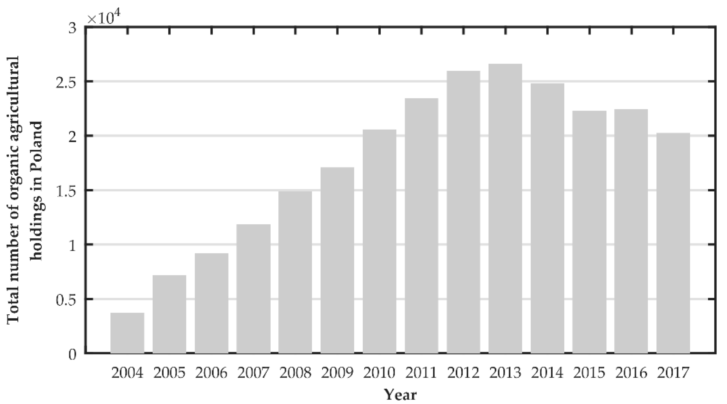
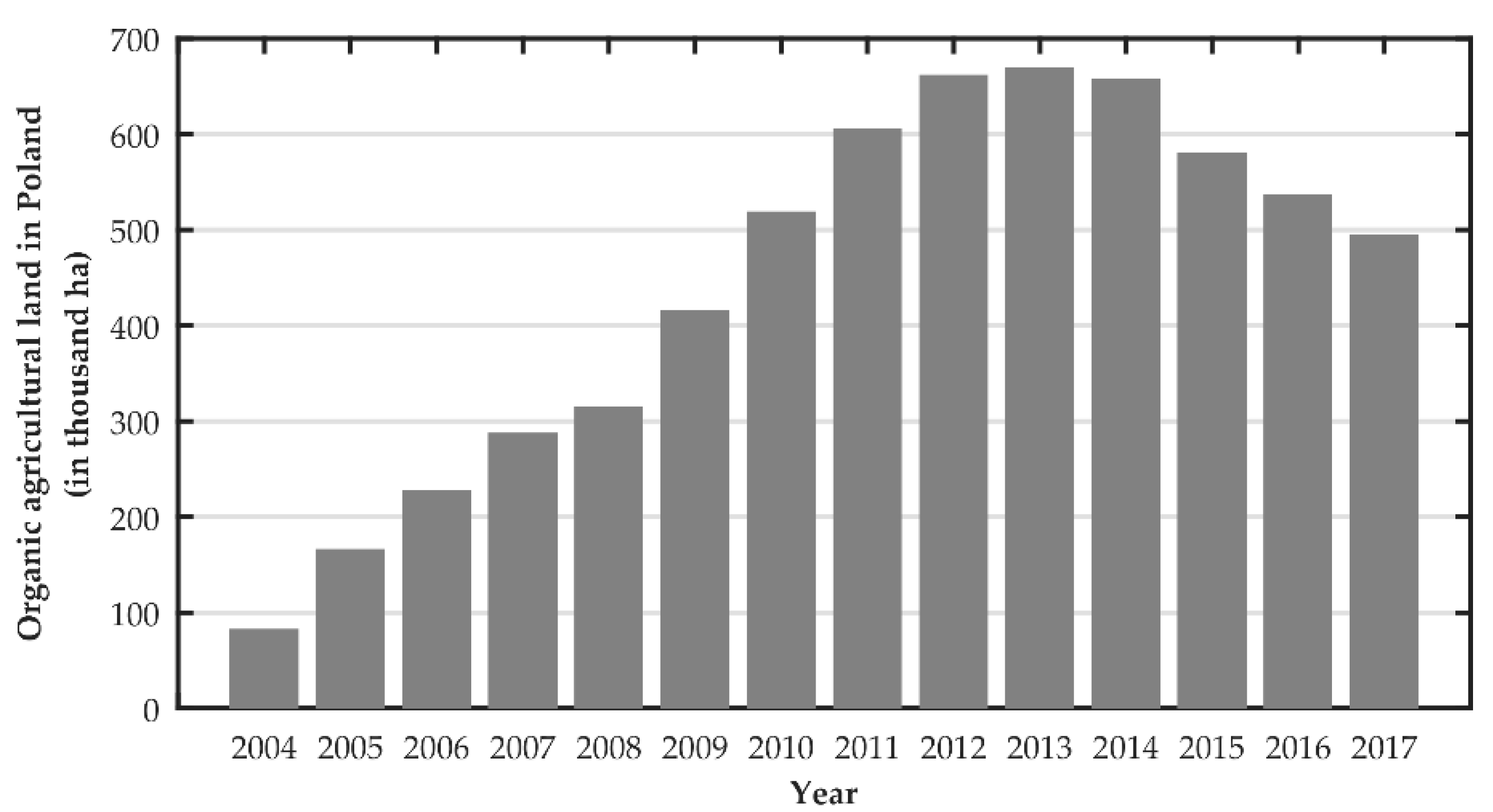
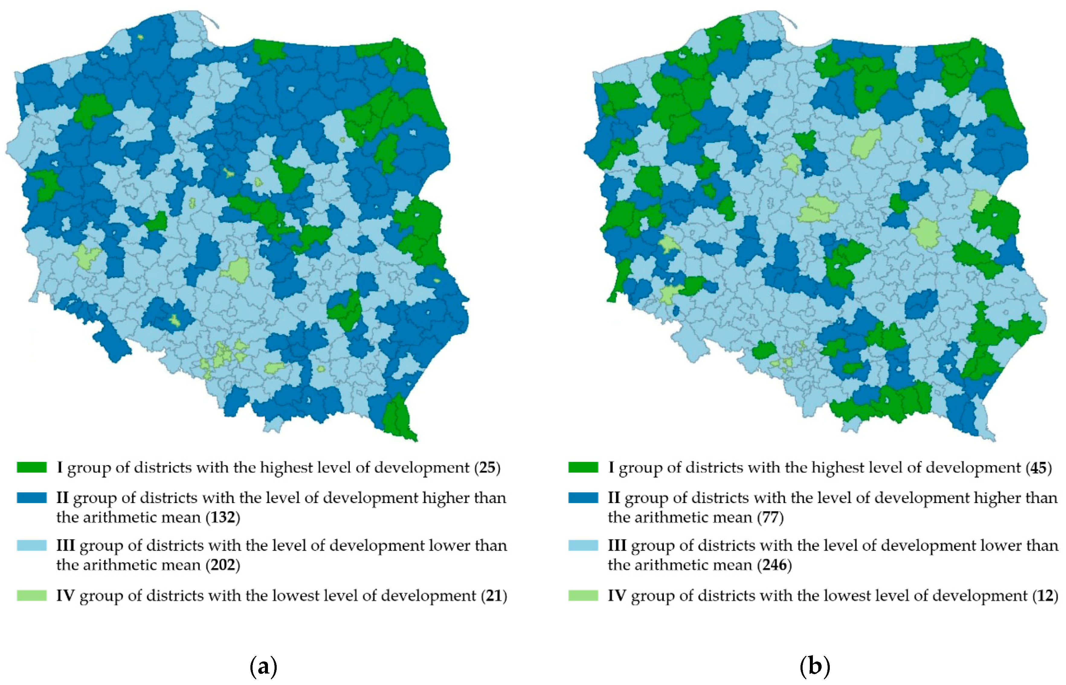
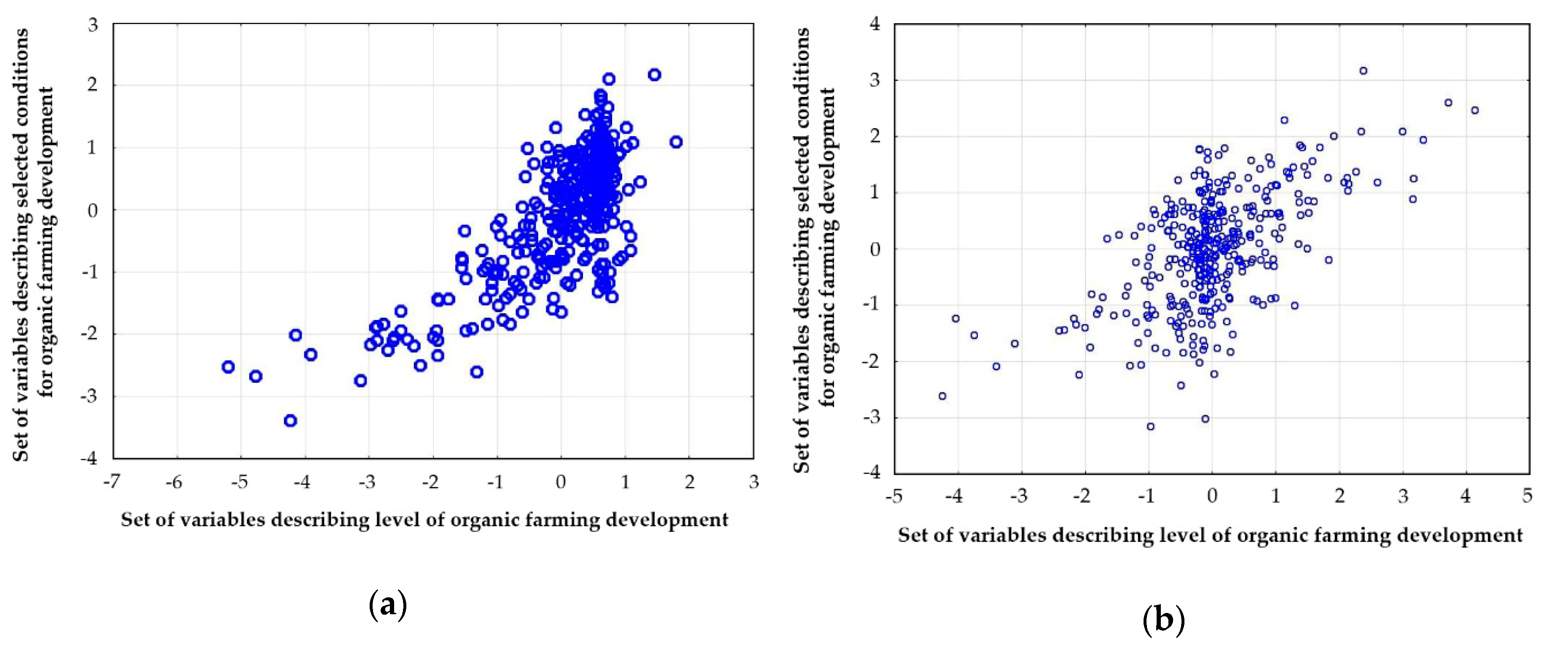